Formulation of Improved Grey Wolf Optimization Methodology for ELD Problem

Available online at www.ijrat.org

Formulation of Improved Grey Wolf

Optimization Methodology for ELD Problem

Guntaas

, Mr.Sushil Prashar

Department Electrical Engineering, D.A.V.I.E.T., Jalandhar, Punjab, India

Email:

[email protected]

, [email protected]

Abstract-In this paper, a new meta-heuristic technique IGWO(Improved Grey Wolf Optimization) is being

formulated to solve Economic Load Dispatch Problem. And the results have been compared with single objective GWO for three unit system with 9 bus-system and for six unit system with 30 bus-system. Furthermore the proposed algorithm obtains competitive performance compared to other proposed techniques.

Index Terms- IGWO (Improved Grey Wolf Optimizer);ELD (Economic Load Dispatch); GWO(Grey Wolf

Optimizer)

1. INTRODUCTION

In power system, the economic load dispatch problem arose when two or more generating units mutually produced the electrical power which goes beyond the required generation. Engineers resolve this problem by executing that how to divide the load among the committed generating units. Two third of the electrical power generated in India is from coal based power stations. The electricity generated from fossil fuel release several pollutants, such as Nitrogen Oxides (NOx), Sulphur Oxides (SOx) and Carbon Dioxide (CO2) into atmosphere. These cause harmful effects to human healthiness and the class of life.. But this load allocation may boost the cost of operation of the generating units. So, it is necessary to find out solutions which give an impartial result among cost and emission. This possibly will be accomplished by Combined Economic Emission Dispatch problem.

Many traditional methods including linear programming method, gradient method, Newton Raphson method and lambda iteration method have been applied to solve ELD problem. The ELD problem has been also solved by the technique of dynamic programming but it suffers from the problem of dimensionality. Some of the meta-heuristic techniques such as differential evolution, particle swarm optimization, tabu search, harmony search, cuckoo search, GWO (Grey Wolf Optimization) have been applied to solve ELD problem. In this paper, a new meta-heuristic technique Improved GWO has been formulated to solve the ELD problem.

2. OBJECTIVE OF ELD

The main objective of the problem of ELD is to minimize the total cost that is generated while satisfying the different constraints, when the required power load is being supplied. The objective function that has to be minimized is given by the following equations:

F(Pg) = ∑ ( aiPgi2 + biPgi + ci)

Where ai, bi, ci are the coefficient of fuel cost of ithgenerator,Rs/MW2 h, Rs/MW h, Rs/h

and F(Pg) is the total fuel cost in Rs/h

The overall fuel cost has to be reduced with the following constraints:

• Power balance constraint: The total generation must be equal to the total power demand and the system’s power losses.

∑

Pgi– Pd- Pl

Where Pl and Pd are the transmission losses and the power demand in MW

• Generator limit constraint: The power generation of each generator has to be controlled within its particular upper and lower operating limits.

∑

Pgimin≤ Pgi≤ Pgimax ;i= 1,2,….ng

Where Pgiminis the minimum limit of generator for ith generator in MW andPgi

max

Available online at www.ijrat.org

GWO algorithm was primarily proposed by Syed Mohammad Mirajili. A grey wolf is characterized by powerful teeth, bushy tail and grey wolves hunt in a pack which has an average group size of 5-12. Their natural habitats are found in the mountains, forests and plains of North America, Asia and Europe. GWO algorithm consists of four models which are as follows:

3.1 Social Hierarchy- The hierarchy of

the grey wolves exist in a pack in which ‘α’ is the leader and the most dominant one & takes the important decisions, ‘β’ and ‘δ’ are subordinates & assists ‘α’ in decision making and the rest are the omega which have to follow the directions given by ‘α’, ‘β’, and ‘δ’.

3.2 Encircling Prey- The mathematical

modelling involved in encircling prey is represented by following equations :

D = | CXp - AX(t) …….(1)

X(t+1) = Xp(t) – AD ……(2)

Where A and C are coefficients vectors given by :

A = 2 a*r1*a ….. (3)

C = 2*r2 ……. (4)

t is the current iteration

X is the position vector of a wolf

r1 and r2 are random vectors € [0,1] and ‘a’ linearly decreases from 2 to 0

3.3 Hunting-The hunting mechanism of

the grey wolves involves the following steps:

Tracking, chasing and approaching the prey.

Pursuing, encircling and harassing the prey until the time it stops moving.

Finally, attacking the prey.

However in abstract search space, we have no idea about the location of the optimum (prey).In order to mathematically simulate the hunting behaviour, we assume that the alpha, beta and delta have better knowledge about the potential location of the prey as follows:

Dα = C1.Xα−X

Dβ= C2.Xβ−X,

Dδ= C3.Xδ−X …. (8)

X1=Xα−A1.(Dα)

X2=Xβ−A2.Dβ

X3=Xδ−A3.(Dδ) ….(9)

X (t+1) = (X1+X2+X3)…(10) 3

Where t is the current iterationandXα, Xβ

and Xδare the position vector of the grey

wolves α , β and δ.

3.4 Attacking prey and search for prey (exploitation and exploration) - The

ability of the grey wolves may result in the global optima; which is the exploitation ability. Since the value of

a decreases from 2 to 0, A is also

simultaneously decreased. A is a random value in the interval [-2a, 2a]. When |A| < 1, the grey wolves are forced to attack the prey. The random values of A are used to indulge the search agent to diverge from the prey. When |A| > 1, the grey wolves are forced to diverge from the prey.

4. AN IMPROVED GREY WOLF

OPTIMIZATION(IGWO) ALGORITHM

The agent’s movement in GWO depends significantly on the circumstances of the alpha, beta and delta. Fig. (1) below shows how a search agent is updating its position. In this paper, we added a new approach to calculate the vectors D՛ α, D՛ β, D՛ δ which

Available online at

D՛ α= | C1. Xr1 – Xr3 |

D՛ β = | C2 . Xr2 – Xr1 |

D_՛ δ = | C3 . Xr3 – Xr1 | …..(11)

X_՛ 1 = Xα – A1 . (D՛ α)

X՛ 2 = Xβ – A2 . (D՛ β)

X՛ 3 = Xδ – A3 . (D՛ δ)…. (12)

X՛ (t + 1) = X՛ 1 + X՛ 2 + X՛ 3 3

The pseudo code of IGWO algorithm has been shown in figure (2), the differences between the standard GWO and the IGWO have been highlighted by “ » ”.

‘Figure (1) showing position of omega ( or any other hunters in GWO & IGWO’

Available online at www.ijrat.org

.(11)

3….(13)

pseudo code of IGWO algorithm has been shown in figure (2), the differences between the standard GWO and the IGWO have been

‘Figure (1) showing position of omega (ω)

or any other hunters in GWO & IGWO’ ‘Figure (2) showing Pseudo

Initialize the grey wolf population X

1,2,…..n )

Initialize a, A and C

Calculate the fitness of each search agent

Xα = the best search agent

Xβ = the second best search agent

Xδ= the third best

While( t< Max number of iterations) for each search agent

» if |A| < 1

» Calculate vectors D

and Dδ by equation (8)

» else

» Calculate vectors D

D՛ β and D՛ δ by equation (11)

» end if

Update the position of the curr

agents by equation (10) or (13) depending upon the selected strategy.

end for

Update a and C by (4) and A is updated by using (3) Calculate the fitness of all search agents

Update X T = t + 1

end while

Return Xα

Figure (2) showing Pseudo- Code of IGWO’ the grey wolf population Xi( i =

e a, A and C

Calculate the fitness of each search agent

= the best search agent

= the second best search agent

= the third best search agent

( t< Max number of iterations)

each search agent

Calculate vectors Dα, Dβ

by equation (8)

Calculate vectors D՛ α,

by equation (11)

Update the position of the current search agents by equation (10) or (13) depending upon the selected strategy.

Update a and C by (4) and A is updated by using (3) Calculate the fitness of all search

Available online at www.ijrat.org

ELD problem involves the following steps:

Step I: Implementation

The main task of ELD is to allocate the load demand among participating generators at minimum possible cost without violating any system constraints. The ED problem is formulated by Eq. (i) and transmission losses are formulated by Eq. (ii)

= ∑ + + (i)

0 00

1 1

n n

L gi ij gj i gi

i i

P

P B P

B P

B

= =

=

∑

+

∑

+

(ii)

Step II: Improved Grey Wolf Pack Representation

Real power generations are the decision variable for ELD problem. Let if there are NG generators in the system, the representation of the wolf position would be described in the form of vector length NG. Let NP wolves are taken in the pack, the representation of complete pack in the matrix form as noted below:

Pack =

…

…

… … …

…

…(iii)

Step III: Pack Initialization

The initialization of each element of above described pack matrix is occurred randomly within capacity constraints depend upon Eq. (iv). The initialization of the wolf positions is done through this inequality:

< <

(i=1,2..NP;j=1,2...NG)……...(iv)

= + −

..(v)

To satisfy energy constraints, one of the committed generators is chosen as a dependent/slack generator d and this is obtained by:

#= $(i=1, 2...NP; j= 1, 2...NG) (vi)

Where

$ = #− ∑,&#… (vii)

If there is the violation of the operating limits by the production of the dependent/slack generator then it is set by equation :

= '

; <

; >

; < <

*

(i=1,2...NG ; i≠ ; j= 1,2..L)..(viii)

After restraining the value of dependent generator, a penalty term is set up in objective function. Therefore the function is defined by:

,₌

. + ∅ … (ix)

Step V: Encircling the prey

The encircling behaviour can be mathematically modelled as follows:

D112 = 3C12. P1127t − P112t 3… (x)

P112t + 1 = P1127t − A112. D112… (xi)

Where A112 and C12 are coefficient vectors, P112₇ is the

prey’s position vector, P112denotes the grey wolf’s position vector and t is the current iteration.

The calculation of vectors A and C is done as follows:

A112 = 2. a12. r2. a12… (xii)

C12 = 2. r2… (xiii)

Available online at

Updating the position

Grey wolves have the capability to identify the position of prey and encircle them. The other wolves must update their positions according to best wolf position. The update of their agent position can be formulated as follows:

D112> 3C12. P112>" P1123 , D112? 3C12. P1 3C12@. P112A" P11

P112 P112>" A112. D112> ,P112 P112_?

A112. -D112?. , P112@ P112A" A112@. D112

P112t 1 P112 P112₃

Position updating of the search agent according to beta, alpha and delta in a two dimensional search space is shown in fig.1 shown above.

IGWO agent position updating:

D′

1112_{> 3C12. P112D" P1111123 , D′D@} 1112_{? 3C12. P1} 3C12@. P112D@" P1111123D

P′

1112 _{P112>" A112. D′}1112_> ,P′1112 P112_?" A112

P112A" A112@. D′1112A

P112′t 1 P′1112 P′1112₃

Step VII: Stopping Criterion

A stochastic optimization approach can be terminated by many criterions at hand. Some of them are maximum no. of iterations, no. of functions evaluations and tolerance. In the present case, maximum no. of iteration is taken for this task.

Available online at www.ijrat.org

Grey wolves have the capability to identify the position of prey and encircle them. The other wolves must update their positions according to best wolf position. The update of their agent

follows:

3 P112?" P1123 , D112A P123

2_?" D2A)

P112@

Position updating of the search agent according to beta, alpha and delta in a two dimensional search

1 shown above.

3 P112D" P1111123 , D′D 1112A 23

2_{. ED′}1112_{?F , P′}1112_@

P′1112@

A stochastic optimization approach can be terminated by many criterions at hand. Some of them are maximum no. of iterations, no. of functions evaluations and tolerance. In the present case, maximum no. of iteration is taken for this

‘Flowchart of IGWO’

5. RESULTS AND DISCUSSIONS:

(ELD with transmission losses) (5.1) Case 1: Three unit system

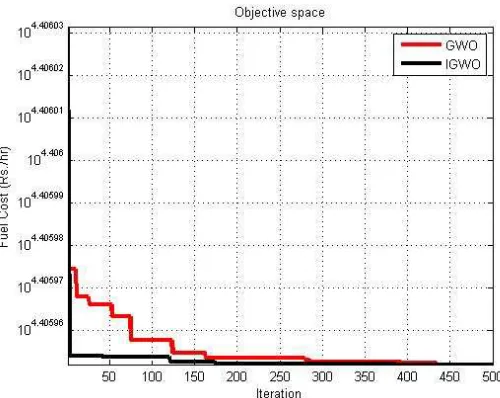
The IGWO algorithm has been implemented on a system consisting of three generator units with transmission loss. The population number is set to 30 and maximum number of iterations performed is 500. The ELD result is shown in table

various columns represent power demand, allocation of loads, power loss and fuel cost. Table 3 shows the comparison of IGWO method with other methods and the convergence curve of fuel cost is shown in the figure 3.

‘Flowchart of IGWO’

RESULTS AND DISCUSSIONS:

(ELD with transmission losses) unit system

The IGWO algorithm has been implemented on a system consisting of three generator units with transmission loss. The population number is set to 30 and maximum number of iterations performed is e ELD result is shown in table 2 in which various columns represent power demand, er loss and fuel cost. Table 3 shows the comparison of IGWO method with other methods and the convergence curve of fuel

Available online at www.ijrat.org

Table 1.Generating unit data for test case I

Bmn G

0.000071 0.000030 0.000025

0.000030 0.000069 0.000032

0.000025 0.000032 0.000080N

Where Bmnis loss coefficient matrix and is derived from reference [18] and also givenin the above table 1

Table 2.ELD using IGW0 for 3-unit system

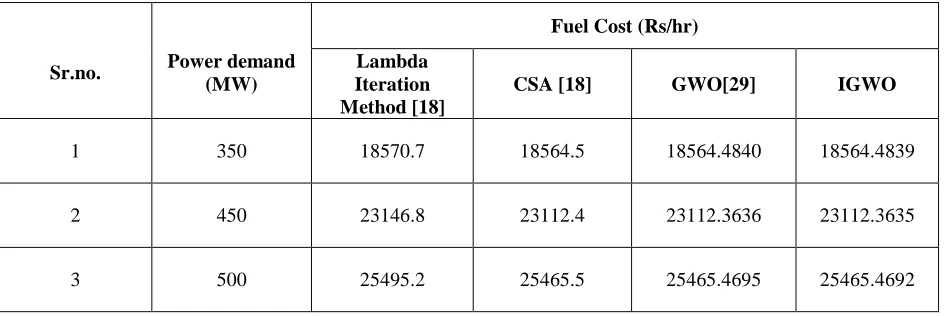
Table 3.Comparison of fuel cost with other techniques for 3-unit system

Sr.no. Power demand (MW)

Fuel Cost (Rs/hr) Lambda

Iteration Method [18]

CSA [18] GWO[29] IGWO

1 350 18570.7 18564.5 18564.4840 18564.4839

2 450 23146.8 23112.4 23112.3636 23112.3635

3 500 25495.2 25465.5 25465.4695 25465.4692

Unit

ai

bi

ci

Pgi

Pgi

1 0.03546 38.30553 1243.5311 35 210

2 0.02111 36.32782 1658.5696 130 325

3 0.01799 38.27041 1356.6592 125 315

Sr.no _Method

Power demand

(MW) P1(MW) P2(MW) P3(MW) PL(MW) Fuel Cost (Rs/hr)

1 GWO

350

70.2909156 156.273451 129.212702 5.77706865 18564.48400014865

IGWO 70.3109238 156.262282 129.203690 5.77689684 18564.48399949439

2 GWO

450

93.9033202 193.782924 171.926898 9.61314331 23112.36364959517

IGWO 93.9385261 193.767679 171.906550 9.61275586 23112.36358629148

3 GWO

500

105.940338 212.627333 193.346108 11.9137811 25465.46954033266

Available online at www.ijrat.org

‘Figure 3 showing convergence curve for three generators for 500 MW demand’

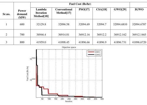
(5.2) Case 2: Six unit system

The IGWO algorithm has been implemented on a test system of six generator units. The ELD result is shown in table 5 in which various columns

represent method used, power demand, allocation of loads, power loss and fuel cost. Table 6 shows the comparison of IGWO method with other methods and the convergence curve of fuel cost is shown in figure 4.

Table 4.Generating unit data for test case II

Unit ai bi ci Pgimin Pgimax

1 0.15240 38.53973 756.79886 10 125

2 0.10587 46.15916 451.32513 10 150

3 0.02803 40.39655 1049.9977 35 225

4 0.03546 38.30553 1243.5311 35 210

5 0.02111 36.32782 1658.5596 130 325

6 0.01799 38.27041 1356.6592 125 315

Bmn=

O P P P P

Q0_{0.000017 0.000060 0.000013 0.000016 0.000015 0.000020}.000014 0.000017 0.000015 0.000019 0.000026 0.000022

0.000015 0.000013 0.000065 0.000017 0.000024 0.000019 0.000019 0.000016 0.000017 0.000072 0.000030 0.000025 0.000026 0.000015 0.000024 0.000030 0.000069 0.000032 0.000022 0.000020 0.000019 0.000025 0.000032 0.000085ST

T T T U

Available online at www.ijrat.org

Table 5.ELD using IGWO for 6-unit system

Sr. No

Method Power Demand

(MW)

P1 (MW)

P2 (MW)

P3 (MW)

P4 (MW)

P5 (MW)

P6 (MW)

PL (MW)

Fuel cost(Rs/h)

1 Conventio nal[17]

600

23.90 10.00 95.63 100.70 202.82 182.02 15.07 32069.58

CS[18] 23.860 10 95.6389 100.708 202.832 181.198 14.2374 32094.7 GWO[29] 23.826 10 95.835 100.727 202.597 181.248 14.2341 32094.681

0 IGWO 23.820 10 95.631 100.749 202.417 181.218 14.2378 32094.678

7 2 Conventio

nal[17]

700

28.33 10.00 118.95 118.67 230.763 212.80 19.50 36914.01

CS[30] 28.351 10.00 118.887 118.675 230.763 212.745 19.4319 36912.2 GWO[29] 28.312 10.003 118.950 119.190 230.252 212.714 19.424 36912.162

0 IGWO 28.235 10.002 118.952 118.628 230.784 212.830 19.434 36912.146

5 3 Conventio

nal[17]

800

32.63 14.48 141.54 136.04 257.65 243.00 25.34 4898.45

CS[18] 32.586 14.484 141.548 136.045 257.664 243.009 25.3309 41896.7 GWO[29] 32.756 13.684 141.925 136.278 257.808 242.893 25.3473

7

41896.708 9 IGWO 32.533 14.305 141.507 135.992 257.841 243.1620 25.3423 41896.634

1

Table 6.Comparison of fuel cost with other techniques for six unit system

Sr.no.

Power demand

(MW)

Fuel Cost (Rs/hr) Lambda

Iteration Method[18]

Conventional Method[17]

PSO[17] CSA[18] GWO[29] IGWO

1 600 32129.8 32096.58 32094.69 32094.7 32094.6810 32094.6787

2 700 36946.4 36914.01 36912.16 36912.2 36912.162 36912.1465

Available online at www.ijrat.org

In this paper, ELD problem has been solved by using IGWO. The results of IGWO are being compared for three and six generating unit system with the other techniques. The algorithm has been programmed in MATLAB(R2009b) software package. The results clearly show effectiveness of IGWO for solving the problem of economic load dispatch. The advantages of IGWO algorithm are simple structure, good reliability, fast convergence, better efficiency for practical applications and also the mechanism of balance between exploration and exploitation ability has been taken into account.

7.REFERNCES

[1] Feng Gao, “Economic Dispatch algorithm for thermal unit system involving combined cycle units”, 15th PSCC, Liege, 22-26 August 2005.

[2] Chiang, Chao-Lung. "Improved genetic algorithm for power economic dispatch of units with valve-point effects and multiple fuels."Power Systems, IEEE Transactions on 20, no. 4 (2005): 1690-1699.

[3] Z.Xue-wen,L.Yan-jun, “ New Algorithm for Economic Load Dispatch of Power Systems.”Institute of Intelligent Systems & Decision Making, Zhejiang University, Hangzhou 310027,2006.

[4] Sudhakaran, M., Ajay-D-Vimal Raj, P., Palanivelu, T.G., "Application of Particle Swarm Optimization for Economic Load Dispatch Problems," Intelligent Systems Applications to Power Systems, 2007. International Conference on, pp.1-7, 5-8 Nov.

2007

[5] Devi, A. Lakshmi, and O. Vamsi Krishna. "combined Economic and Emission dispatch using evolutionary algorithms-A case study."

ARPN Journal of engineering and applied sciences 3, no. 6 (2008): 28-35.

[6] Dhillon, J.S., Kothari, D.P. , "Economic-emission load dispatch using binary successive approximation-based evolutionary search,"

Generation, Transmission & Distribution, IET

, vol.3, no.1, pp.1-16, January 2009

[7] Kumar, K. Sathish, R. Rajaram, V. Tamilselvan, V. Shanmugasundaram, S.

Naveen, and IG Mohamed NowfalHariharan T. Jayabarathi. "Economic dispatch with valve point effect using various PSO Techniques." Vol 2, No. 6, (2009):130-135

[8] Bhattacharya, Aniruddha, and Pranab Kumar Chattopadhyay. "Solving complex economic load dispatch problems using biogeography-based optimization."Expert

Systems with Applications 37, no. 5 (2010):

3605-3615.

[9] Bhattacharya, Aniruddha, and P. K. Chattopadhyay. "Application of biogeography-based optimization for solving multi-objective economic emission load dispatch problems."Electric Power Components and

Systems 38, no. 3 (2010): 340-365.

[10] AnantBaijal, Vikram Singh Chauhanand T Jayabarathi,” Application of PSO, Artificial Bee Colony and Bacterial Foraging Optimization algorithms to economic load dispatch: An analysis” IJCSI International Journal of Computer Science Issues, Vol. 8, Issue 4, No 1, July 2011.

[11] Rayapudi, S. Rao. "An intelligent water drop algorithm for solving economic load dispatch problem." International Journal of

Electrical and Electronics Engineering 5, no. 2

(2011): 43-49.

[12] TheofanisApostolopoulos and Aristidis Vlachos,” Application of the Firefly Algorithm for Solving the Economic Emissions Load Dispatch Problem”International Journal of Combinatorics Volume 2011

[13] Swain, R. K., N. C. Sahu, and P. K. Hota. "Gravitational search algorithm for optimal economic dispatch."Procedia Technology 6 (2012): 411-419.

[14]Yang, Xin-She, SeyyedSoheil Sadat Hosseini, and Amir Hossein Gandomi."Firefly algorithm for solving non-convex economic dispatch problems with valve loading effect."Applied Soft Computing 12, no. 3 (2012): 1180-1186.

[15] Surekha P, Dr.S.Sumathi,” Solving Economic Load Dispatch problems using Differential Evolution with Opposition Based Learning” WSEAS TRANSACTIONS on

Available online at www.ijrat.org

APPLICATIONS, Issue 1, Volume 9, January 2012.

[16] Güvenç, U., Y. Sönmez, S. Duman, and N. Yörükeren. "Combined economic and emission dispatch solution using gravitational search algorithm." Scientia Iranica 19, no. 6 (2012): 1754-1762

[17] Yohannes, M. S. "Solving economic load

dispatch problem using particle swarm optimization technique." International Journal

of Intelligent Systems and Applications (IJISA) 4, no. 12 (2012): 12.

[18] Bindu, A. Hima, and M. Damodar Reddy. "Economic Load Dispatch Using Cuckoo

Search Algorithm." Int. Journal Of Engineering

Research and Apllications 3, no. 4 (2013): 498-502.

[19] R Subramanian, K. Thanushkodi and A. Prakash, “An efficient Meta Heuristic Algorithm to Solve Economic Load Dispatch Problems”. Iranian Journal of Electrical and Electronics Engineering. Vol. 9, No.4 Dec 2013.

[20] Wang, Ling, and Ling-po Li. "An effective differential harmony search algorithm for the solving non-convex economic load dispatch problems." International Journal of

Electrical Power & Energy Systems 44, no. 1

(2013): 832-843.

[21] Shubham Tiwari, Ankit Kumar, G.S Chaurasia, G.S Sirohi,” Economic Load Dispatch Using Particle Swarm Optimization” IJAIEM, Volume 2, Issue 4, April 2013.

[22] Ravi, C. N., and Dr C. ChristoberAsirRajan. "Differential Evolution technique to solve Combined Economic Emission Dispatch." In 3rd International

Conference on Electronics, Biomedical

Engineering and its Applications (ICEBEA'2013) January, pp. 26-27. 2013.

[23] Xin-She Yang, Xingshi He,” Firefly Algorithm: Recent Advances and Applications” arXiv:1308.3898v1, 18 Aug 2013

[24] Kherfane, R. L., M. Younes, N. Kherfane, and F. Khodja. "Solving Economic Dispatch Problem Using Hybrid GA-MGA."Energy

Procedia 50 (2014): 937-944.

[25] Aydin, Dogan, SerdarOzyon, CelalYaşar, and Tianjun Liao. "Artificial bee colony algorithm with dynamic population size to combined economic and emission dispatch problem." International journal of electrical

power & energy systems 54 (2014): 144-153.

[26] Thao, Nguyen Thi Phuong, and Nguyen Trung Thang. "Environmental Economic Load Dispatch with Quadratic Fuel Cost Function Using Cuckoo Search Algorithm."

International Journal of u-and e-Service, Science and Technology 7, no. 2 (2014):

199-210.

[27] Mirjalili, Seyedali, Seyed Mohammad Mirjalili, and Andrew Lewis. "Grey wolf optimizer." Advances in Engineering Software 69 (2014): 46-61.

[28] NipotepatMuangkote, KhamronSunat, SirapatChiewchanwattana, “An Improved Grey Wolf Optimizer for Training q-Gaussian Radial Basis Functional-link Nets”,International Computer Science and

Engineering Conference (ICSEC),2014

[29] Dr.Sudhir Sharma, Shivani Mehta, Nitish Chopra,” Economic Load Dispatch Using Grey Wolf Optimization”, International Journal of