Capacitated arc routing problem with time window in solid waste operation

3

CAPACITATED ARC ROUTING

PROBLEM WITH TIME WINDOW IN

SOLID WASTE OPERATION

Zuhaimy Hj. Ismail

Mohammad Fadzli Raml

i

3.1 OVERVIEW

In most countries, waste collection problems are frequently considered as environmental and pollution issues thus many approaches have been carried out onto development of policies and improving of waste management at administration level. On the contrary, very few researches have been done to improve the service of waste collection to customers instead. Compared to well-known VRP, CARP has been neglected for a long time, but has a growing interest in two last decades, mainly because its important applications in waste collection, inspection of power lines, and winter gritting.

3.2 PROBLEM IDENTIFICATION

3.2.1 CASE STUDY

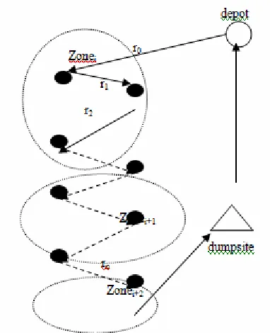
Our case study and data collection has been carried out onto Syarikat Perniagaan Zawiyah Sdn. Bhd., a waste collection contractor appointed by MBJB. Our observation took place in Zone 6 and Zone 7 Taman Setia Indah and Taman Kempas Indah, Johor Bahru. The operation trip of one identical truck starts everyday from workshop depot at Tampoi to the nearest collection zone then to dumpsite area at Seelong (Figure 3.1). Dumpsite will be closed at 5pm everyday due to security reason, so collection of waste must be completed before 4pm, as traveling time to the dumpsite approximately is 45 minutes.

Figure 3.1. Conceptual model of truck operation in solid waste operation.

3.3 FORMULATION OF CARPTW

The CARP formulated by Dror and Langevin [8] is as follows. Given a connected graph G = (V, E ∪A), with V as the set of nodes (vertices), E set of edges (E V x V) and A a set of arcs (A V x V), the objective of the problem is to find a minimum cost traversal of a given subset of edges and arcs in R E A. The CARP has an additional traversal cost for each edge and arc with edge (arc) demand q

⊆ ⊆

⊆ ∪

ij 0 for each edge (i, j) which must be serviced by one of a fleet of vehicles of capacity W. The problem is to find a number of circuits each of which passes through the depot which satisfies demands at minimal total cost.

We denote cij as the cost of an edge (arc) (i, j) ∈ E(A) and xijk as the number of times edge (arc) (i, j) ∈ E A is traversed in trip k.

∪

yijk = 1 if the edge (arc) (i, j)∈R is covered in trip

k;

0 otherwise.

M is a large constant greater than or equal to the sum of traversals of edges and arcs in a given S R, V[S] is the set of nodes incident to the arc set S, k denotes a trip, and K is the maximum number of trips allowed.

⊆

The objective function seeks to minimize total cost, and it is given as follows:

Minimize

∑ ∑

fc ) , ( 1 ) ( 1 1 K ijk k y = =

∑

, ijk ijk y

x ≥ ∀(i, j)∈R, for k = 1, 2,..,K

∑

q

) , (

, for k = 1, 2,…, K

yijk∈{0,1} ∀(i, j)∈R, k = 1, 2, …,K

xijk ∈Z+ ∀(i, j)∈E, k = 1, 2, …,K

household. Equation (3.1) ensures route discrete continuity. Equation (3.2) state that each edge with positive demand is serviced exactly once. Equation (3.3) guarantees that the traversal circuit k covers the edge (i, j)∈ R if it delivers its demand. Vehicle capacity is not violated on account of equation (3.4). Integrality restrictions are given in Equation (3.5) and (3.6).

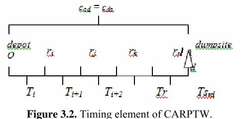
Expansion of timing element in CARPTW as depicted in Figure 3.2. If T is total operation time then T ≤ A, where A is a constant maximum service time. This inequation ensures the service times is not exceed the reasonable operation time before traveling to the dumpsite. Then, Tsrn = B, where B is stochastic traveling time. Moreover, zero demands and service times are defined for this two nodes, that is, d0 = dr0 = s0 = sr0= 0.

Figure 3.2. Timing element of CARPTW.

3.4 HEURISTIC METHOD FOR THE INITIAL SOLUTION

3.4.1 NOTATIONS

Given the inherent computational difficulty of the routing problem, a variety of heuristics have been reported e.g. [9], [10] and [11], mostly for the hard time window. We implemented nearest procedure in order to find the first service route after traveling from the depot. Notations of variables are as follows:

(1) yinit = 0, number of routes before first cycle starts.

(2) qinit = 0, initial capacity for one vehicle before first

cycle starts.

(3) cinit = 0, initial cost for one vehicle before first cycle

starts.

(4) cij , cost from point i to point j ,

Ei+1 , next successor edge ,

y = yinit + 1, count of routes after each cycle starts.

(5) qnew = qinit + qij , capacity at route ij,

(6) qbalnew = q – qnew , balance of capacity after collection

at route ij.

(7) cnew = cinit + cij , sum of route cost from depot to point i

to point j.

(8) c=cinit+cnew, increase of cost with increse the number of

routes.

(9) qnew:= , sum of capacity from point i to point n,

assigned to capacity variable.

∑

+ n

i q

i 1

(10) qbalnew := q - , balance capacity from point i to

point n, assigned to balance capacity variable.

∑

+ n

i q

i 1

(11) cnew :=

∑

(12) qinit := qnew , new capacity reassign to initial capacity

after each cycle.

(13) cinit := cnew , new cost reassign to initial cost after each

cycle.

(14) qbalnew≥ q , decision operator for capacity.

3.4.2 NEAREST PROCEDURE

Nearest procedure build a feasible solution by inserting at every iteration an unrouted customer into a previous continuity serviced routes. This process is performed one route a time.

Step 1: Input V and E. Set depot O = initial, yinit = 0, qinit = 0, cost Cinit = 0, capacity q = W, trip k = 0.

Step 2: From O, k := k + 1, find the successor customer, Vi, compare and choose nearest j and Ei+1. Set y = yinit + 1, count new weight, qnew = qinit + qi and qbalnew = W – qnew. Count new cost, cnew = cinit + cij.

Step 3: If qbalnew < W, then check the next successor, Vi+1. Assigned qnew :=

and q

∑

= + n

i q

i 1 balnew := W -

∑

= + n

i q

i 1 new :=

∑

:= Qnew and Cinit := Cnew. If Qbalnew≥ Q. Assigned yinit := y. Terminate

all served edges and go to Step 1.

Step 4: Repeat Step 1 until all served y = V. Void all served y. Count assigned pre-edges cost.

3.5 CONCLUSION

evaluation for this model. More robust algorithms must be prepared, appropriate lower bound must be developed, while no other algorithm is available for comparison. All these tasks are in progress.

3.6 REFERENCES

[1] J-M. Belenguer, E. Benavent, P. Lacomme, and C. Prins, “Lower and upper bounds for the mixed capacitated arc routing problem”, Computers & Operations Research 33, Elsevier Ltd, 2006, pp. 3363–3383.

[2] J. Bautista, E. Fernandez, and J. Pereira, “Solving an urban waste collection problem using ants heuristics”, Computers & Operations Research 35, Elsevier Ltd, 2008, 2008, pp. 3020-3033.

[3] M. C. Mourao, L.S.Pinto, and L.Gouveia, “Modeling capacitated arc-routing problems”, Optimization2007. 23-24 July 2007. Portugal.

[4] F. Chu, N. Labadi, and C. Prins, “A scatter search for the periodic capacitated arc routing problem”, European Journal of Operational Research 169, Elsevier B. V., 2006, pp. 586-605.

[5] P. Lacomme, C. Prins, and R-C. Wahiba, “Evolutionary algorithms for periodic arc routing problems”, European Journal of Operational Research 165, Elsevier B. V., 2005, pp. 535-553.

[6] G. Fleury, P. Lacomme, C. Prins, and R-C. Wahiba, “Improving robustness of solutions to arc routing problems”, The Journal of the Operational Research Society 56, Palgrave, 2005, pp. 526-538.

routing problem”, Proceedings of IEEE, International Conference of Automation and Logistics, 18-21 August 2007, Jinan, China.

[8] M. Dror, and A. Langevin, “Transformation and exact node routing solutions by column generation”, Arc Routing: Theory, Solutions and Applications, Kluwer Academic Publishers, Dordrecht, 2000, pp. 277–326.

[9] M.W.P. Savelsbergh, “Local search in routing problems with time windows”, Annals of Operations Research 4, 1985, pp. 285-305.

[10] J. Schulze and T. Fahle, “A parallel algorithm for the vehicle routing problem with time window constraints”, Annals of Operations Research 86, 1999, pp. 585-607.