ABSTRACT
CAMERINO, MICHAEL Damage Localization From Sensor and Actuator Data. (Under the direction of Assistant Professor Kara Peters).
Damage Localization From Sensor and Actuator Data
by
Michael J. Camerino
A thesis submitted to the Graduate Faculty of North Carolina State University
in partial satisfaction of the requirements for the Degree of
Master of Science
Department of Mechanical and Aerospace Engineering
Raleigh 2003
Approved By:
Dr. F. G. Yuan
Dr. Jeffrey W. Eischen Dr. Kara Peters
Biography
Acknowledgements
The author would like to acknowledge the support of the North Carolina Space Grant Consortium who funded the data acquisition system used in the experiments and supplying the author with a fellowship for the summer of 2003. I would like to thank Dr. Kara Peters for all the help she has given to me for the last two years. I would like to thank Michel “Bobby” Studer for everything he did for me while he was at North Carolina State University. I would like to thank Mohanraj Prabhugoud as he allowed me to ask him a lot of questions. I would also like to thank Rufus “Skip” Richardson and Mike Breedlove for machining all the equipment used in the experimental work. Finally, I would like to thank my family, mom, Mary Sara, Roy and Matt for all the support they have given me for the last year.
Table of Contents
LIST OF FIGURES
VII
LIST OF TABLES
XVII
1 INTRODUCTION
1
2 BACKGROUND
3
2.1 Damage identification . . . 3
2.2 Current damage detection methods . . . 4
2.2.1 Frequency response methods . . . 4
2.2.2 Model comparison methods . . . 5
2.2.3 Neural Networks . . . 5
2.3 Flexibility approach to damage localization . . . 6
2.4 Application of displacement sensors to the flexibility approach . . . 8
2.5 Truss example . . . 9
2.6 Fiber optic waveguides . . . 13
2.6.1 Introduction to fiber optic waveguides . . . 13
2.6.2 Advantages of fiber optic sensors . . . 14
2.6.3 Fiber Bragg grating strain sensor . . . 16
3 SIMULATIONS
20
3.1 Eight sensor plate model . . . 20
3.1.1 Model explanation . . . 20
3.1.2 Calculation of a flexibility matrix . . . 22
3.1.3 Damage localization . . . 22
3.1.4 Filtering unidentified stress regions . . . 32
3.1.5 Results for damage applied in section 1 . . . 34
3.1.6 Damage applied in section 3 . . . 39
3.1.7 Damage applied in section 7 . . . 40
3.1.8 Damage applied in section 5 . . . 42
3.1.9 Damage applied in sections 1 and 2 . . . 44
3.1.10 Severity of damage . . . 46
3.1.11 Summary of results from the eight sensor model . . . 50
3.2 Thirty-two sensor plate model . . . 50
3.2.2 Damage location for thirty-two sensor plate model . . . 52
3.2.3 Locating damage directly from the DLVs . . . 59
3.2.4 Locating damage using DLVs covering two sections . . . 67
3.2.5 Severity of damage . . . 70
3.2.6 Progressive damage . . . 73
3.2.7 Summary of results from the thirty-two sensor plate . . . 74
4 EXPERIMENTAL WORK
76
4.1 Experimental setup . . . 76
4.1.1 Fiber optic displacement senors . . . 76
4.1.2 Plate and loading frame . . . 80
4.1.3 Data acquisition system . . . 81
4.1.4 Experimental procedure . . . 82
4.2 Results . . . 84
4.2.1 Results of damage applied in the top left section . . . 85
4.2.2 Results of damage applied in the middle of the plate . . . 87
4.3 Summary of results . . . 89
5 CONCLUSIONS
90
6 REFERENCES
92
A APPENDIX: EIGHT SENSOR PLATE PLOTS
94
A.1 Location plots for applied damage in section 3 . . . 94
A.2 Location plots for applied damage in section 7 . . . 98
A.3 Location plots for applied damage in between sections 1 and 2 . 101
A.4 Location plots for applied damage for severity . . . 103
B APPENDIX: THIRTY-TWO SENSOR PLATE PLOTS
108
B.1 Location plots for applied damage in section 8 . . . 108
B.2 Location plots for applied damage in section 9 . . . 110
B.3 Location plots for applied damage in section 11 . . . 113
B.4 Location plots for applied damage in section 12 . . . 115
B.5 Location plots for applied damage in section 13 . . . 117
B.6 Location plots for applied damage in section 14 . . . 120
B.7 Location plots for applied damage in section 15 . . . 122
B.9 Location plots for applied damage in sections 7 damage size 2 . 128
B.10 Location plots for applied damage in sections 7 damage size 3 131
B.11 Location plots for applied damage in sections 7 damage size 4 134
B.12 Location plots for applied damage in sections 7 damage size 5 137
B.13 Location plots for applied damage in sections 7 damage size 6 140
B.14 Progressive damage plate for applied damage in section 7 followed
by damage in section 8 . . . 143
B.15 Progressive damage plate for applied damage in section 7 followed
by damage in section 9 . . . 145
C APPENDIX: TECHNICAL DRAWINGS FOR THE
List of Figures
2
Background
2.1 Schematic illustration of damaged and undamaged domains [8]. . . 6
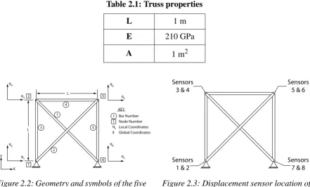
2.2 Geometry and symbols of the five bar truss structure. . . 10
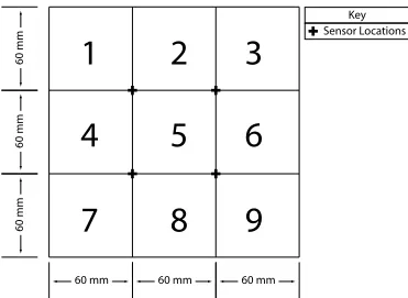
2.3 Displacement sensor location of the five-bar truss. . . 10
2.4 Fiber optic waveguide [13]. . . 13
2.5 Snell’s law applied to a fiber optic waveguide. . . 14
2.6 Three electrical strain gages vs. three fiber optic strain gages. . . 16
2.7 Fiber Bragg grating showing schematically the periodic change in the index of refraction. . . 17
2.8 Phase mask setup for the fabrication of a fiber Bragg grating [16]. . . 17
2.9 Propagation of light waves through an optical fiber with a FBG. . . 18
2.10 Original reflected spectrum from a FBG . . . 18
2.11 FBG spectrum after compressive load has been applied. . . 19
2.12 FBG spectrum after tensile load has been applied. . . 19
3
Simulations
3.1 Dimensions and boundary conditions for the eight sensor plate model. . . 213.2 Sensor locations for the eight sensor plate model. . . 21
3.3 Creation of the undamaged flexibility matrix from displacements at sensors 1 & 2. 23 3.4 Creation of the undamaged flexibility matrix from displacements at sensors 3 & 4. 24 3.5 The nine damage sections of the eight sensor plate model. . . 25
3.6 DLVs for damage in section 1. . . 27
3.7 Application of damage location vector # 1 utilizing a precision of 1. All the forces applied are in N. . . 28
3.8 Maximum principal stress (MPS) plots for locating damage in section 1 utilizing a precision of 1. . . 29
3.9 Damage located using MPS for applied damage in section 1 and a precision of 1. . 31
3.10 Final damage located using MPS for applied damage in section 1 utilizing a precision of 1. . . 32
3.11 Unidentified stress points for MPS for loading schemes one and two. . . 33
3.12 Unidentified stress region for the eight-sensor plate model. . . 33
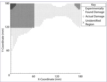
3.13 Location of damage for applied damage in section 1 utilizing a precision of 1 with unidentified areas. . . 34
3.14 Location of damage for applied damage in section 1 utilizing a precision of 2 (producing 7 DLVs). . . 35
3.16 Location of damage for applied damage in section 1 utilizing a precision of 4
(producing 4 DLVs). . . 36
3.17 Location of damage for applied damage in section 1 utilizing a precision of 5 (producing 3 DLVs). . . 36
3.18 Location of damage for applied damage in section 1 utilizing a precision of 6 (producing 2 DLVs). . . 37
3.19 Location of damage for applied damage in section 1 utilizing a precision of 7 (producing 1 DLVs). . . 37
3.20 Location of damage for applied damage in section 3 utilizing a precision of 5 (producing 3 DLVs). . . 39
3.21 Location of damage for applied damage in section 7 utilizing a precision of 5 (producing 3 DLVs). . . 41
3.22 Location of damage for applied damage in section 5 utilizing a precision of 2 (producing 7 DLVs). . . 43
3.23 Location of damage for applied damage in section 5 utilizing a precision of 3 (producing 1 DLV). . . 43
3.24 Applied damage regions located between sections 1 and 2. . . 44
3.25 Location of damage for damage applied in sections 1 and 2 utilizing a precision of 4 (producing 5 DLVs). . . 45
3.26 Location of damage for applied damage in sections 1 and 2 utilizing a precision of 5 (producing 2 DLVs). . . 46
3.27 Location of damage for applied damage in section 1 of dimensions 30 mm x 30 mm utilizing 3 DLVs. . . 49
3.28 Location of damage for applied damage in section 1 of dimensions 3 mm x 3 mm utilizing 3 DLVs. . . 49
3.29 Dimensions and sensor layout for the thirty-two sensor plate. . . 51
3.30 The sixteen damage sections of the thirty-two sensor plate model. . . 52
3.31 Unidentified stress regions located for the thirty-two sensor plate. . . 54
3.32 Location of damage for applied damage in section 1 utilizing a precision of 10 (producing 5 DLVs). . . 54
3.33 Location of damage for applied damage in section 2 utilizing a precision of 11 (producing 9 DLVs). . . 55
3.34 Location of damage for applied damage in section 3 utilizing a precision of 10 (producing 13 DLVs). . . 55
3.35 Location of damage for applied damage in section 4 utilizing a precision of 11 (producing 3 DLVs). . . 56
3.36 Location of damage for applied damage in section 5 utilizing a precision of 11 (producing 5 DLVs). . . 56
3.37 Location of damage for applied damage in section 6 utilizing a precision of 10 (producing 5 DLVs). . . 57
3.38 Location of damage for applied damage in section 7 utilizing a precision of 10 (producing 9 DLVs). . . 57
3.40 Location of damage for applied damage in section 9 utilizing a precision of 10
(producing 8 DLVs). . . 58
3.41 Location of damage for applied damage in section 10 utilizing a precision of 11 (producing 3 DLVs). . . 59
3.42 Sensor occurrence for applied damage in section 7 utilizing 22 DLVs. . . 61
3.43 Sensor occurrence for applied damage in section 7 utilizing 20 DLVs. . . 61
3.44 Sensor occurrence for applied damage in section 7 utilizing 17 DLVs. . . 62
3.45 Sensor occurrence for applied damage in section 7 utilizing 15 DLVs. . . 62
3.46 Sensor occurrence for applied damage in section 7 utilizing 14 DLVs. . . 62
3.47 Sensor occurrence for applied damage in section 7 utilizing 11 DLVs. . . 63
3.48 Sensor occurrence for applied damage in section 7 utilizing 9 DLVs. . . 63
3.49 Sensor occurrence for applied damage in section 8 utilizing 6 DLVs. Sensors 3,4,5,6,11,12,13,14 are closest to damage area. . . 64
3.50 Sensor occurrence for applied damage in section 9 utilizing 8 DLVs. Sensors 1,2,3,4,9,10,11,12 are closest to damage area. . . 64
3.51 Sensor occurrence for applied damage in section 11 utilizing 7 DLVs. Sensors 13,14,15,16,21,22,23,24 are closest to damage area. . . 65
3.52 Sensor occurrence for applied damage in section 12 utilizing 4 DLVs. Sensors 11,12,13,14,19,20,21,22 are closest to damage area. . . 65
3.53 Sensor occurrence for applied damage in section 13 utilizing 6 DLVs. Sensors 9,10,11,12,17,18,19,20 are closest to damage area. . . 65
3.54 Sensor occurrence for applied damage in section 14 utilizing 9 DLVs. Sensors 21,22,23,24,29,30,31,32 are closest to damage area. . . 66
3.55 Sensor occurrence for applied damage in section 15 utilizing 6 DLVs. Sensors 19,20,21,22,27,28,29,30 are closest to damage area. . . 66
3.56 Sensor occurrence for applied damage in section 16 utilizing 8 DLVs. Sensors 17,18,19,20,25,26,27,28 are closest to damage area. . . 66
3.57 Sensor occurrence for applied damage in sections 7 and 8 utilizing 2 DLVs. . . 67
3.58 Sensor occurrence for applied damage in sections 7 and 8 utilizing 3 DLVs. . . 68
3.59 Sensor occurrence for applied damage in sections 7 and 8 utilizing 5 DLVs. . . 68
3.60 Sensor occurrence for applied damage in sections 7 and 8 utilizing 7 DLVs. . . 68
3.61 Sensor occurrence for applied damage in sections 7 and 8 utilizing 10 DLVs. . . 69
3.62 Sensor occurrence for applied damage in sections 7 and 8 utilizing 12 DLVs. . . 69
3.63 Sensor occurrence for applied damage in sections 7 and 8 utilizing 15 DLVs. . . 69
3.64 Sensor occurrence for applied damage in sections 7 and 8 utilizing 18 DLVs. . . 70
3.65 Damage sizes for the thirty-two sensor plate model to test for severity. . . 71
3.66 Occurrence of sensors for applied damage in section 7 size 2 (refer to Figure 3.65) utilizing 4 DLVs . . . 71
3.67 Occurrence of sensors for applied damage in section 7 size 3 (refer to Figure 3.65) utilizing 17 DLVs . . . 72
3.68 Occurrence of sensors for applied damage in section 7 size 4 (refer to Figure 3.65) utilizing 13 DLVs . . . 72
3.70 Occurrence of sensors for applied damage in section 7 size 6 (refer to Figure 3.65)
utilizing 27 DLVs . . . 73
3.71 Occurrence of sensors for progressive damage in section 7 in order to locate damage in section 8 utilizing 1 DLV. . . 74
3.72 Occurrence of sensors for progressive damage in section 7 in order to locate damage in section 9 utilizing 1 DLV. . . 74
4
Experimental Work
4.1 Fiber optic displacement sensors using FBGs. . . 774.2 Three dimensional view of the experimental setup. . . 79
4.3 Sketch of plate including sensors and loading hole locations. . . 80
4.4 Photograph of the plate used in the experiment. . . 81
4.5 Data acquisition system for measuring FBG spectrums in reflection. . . 81
4.6 Photograph of the experimental setup. . . 82
4.7 Four damage cases applied to in the aluminum plate. . . 84
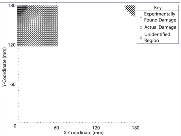
4.8 Damage located for nine holes applied in the top left corner. . . 86
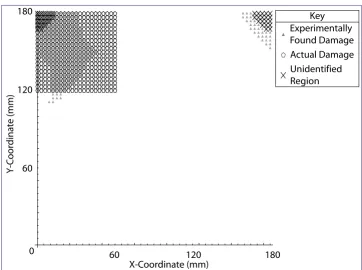
4.9 Damage located for twenty-five holes applied in the top left corner. . . 86
4.10 Damage located for sixty-one holes applied in the top left corner. . . 87
4.11 Damage located for thirty-six holes applied in the middle of the plate. . . 89
A
Appendix: Eight Sensor Plate Plots
A.1 Location of damage for applied damage in section 3 utilizing a precision of 1 (producing 8 DLVs). . . 94A.2 Location of damage for applied damage in section 3 utilizing a precision of 2 (producing 7 DLVs). . . 95
A.3 Location of damage for applied damage in section 3 utilizing a precision of 3 (producing 6 DLVs). . . 95
A.4 Location of damage for applied damage in section 3 utilizing a precision of 4 (producing 4 DLVs). . . 96
A.5 Location of damage for applied damage in section 3 utilizing a precision of 6 (producing 2 DLVs). . . 96
A.6 Location of damage for applied damage in section 3 utilizing a precision of 7 (producing 1 DLVs). . . 97
A.7 Location of damage for applied damage in section 7 utilizing a precision of 2 (producing 7 DLVs). . . 98
A.8 Location of damage for applied damage in section 7 utilizing a precision of 3 (producing 5 DLVs). . . 99
A.9 Location of damage for applied damage in section 7 utilizing a precision of 4 (producing 4 DLVs). . . 99
A.11 Location of damage for applied damage in between sections 1 and 2 utilizing a
precision of 2 (producing 6 DLVs). . . 101 A.12 Location of damage for applied damage in between sections 1 and 2 utilizing a
precision of 3 (producing 5 DLVs). . . 102 A.13 Location of damage for applied damage in between sections 1 and 2 utilizing a
precision of 6 (producing 1 DLVs). . . 102 A.14 Location of damage for applied damage in section 1 of dimensions 54 mm x 54 mm
utilizing 3 DLVs. . . 103 A.15 Location of damage for applied damage in section 1 of dimensions 48 mm x 48 mm
utilizing 3 DLVs. . . 104 A.16 Location of damage for applied damage in section 1 of dimensions 42 mm x 42 mm
utilizing 3 DLVs. . . 104 A.17 Location of damage for applied damage in section 1 of dimensions 36 mm x 36 mm
utilizing 3 DLVs. . . 105 A.18 Location of damage for applied damage in section 1 of dimensions 24 mm x 24 mm
utilizing 3 DLVs. . . 105 A.19 Location of damage for applied damage in section 1 of dimensions 18 mm x 18 mm
utilizing 3 DLVs. . . 106 A.20 Location of damage for applied damage in section 1 of dimensions 12 mm x 12 mm
utilizing 3 DLVs. . . 106 A.21 Location of damage for applied damage in section 1 of dimensions 6 mm x 6 mm
utilizing 3 DLVs. . . 107
B
Appendix: Thirty-two Sensor Plate Plots
B.1 Sensor occurrence for applied damage in section 8 utilizing 8 DLVs. Sensors
3,4,5,6,11,12,13,14 are closest to damage area. . . 108 B.2 Sensor occurrence for applied damage in section 8 utilizing 10 DLVs. Sensors
3,4,5,6,11,12,13,14 are closest to damage area. . . 108 B.3 Sensor occurrence for applied damage in section 8 utilizing 12 DLVs. Sensors
3,4,5,6,11,12,13,14 are closest to damage area. . . 109 B.4 Sensor occurrence for applied damage in section 8 utilizing 15 DLVs. Sensors
3,4,5,6,11,12,13,14 are closest to damage area. . . 109 B.5 Sensor occurrence for applied damage in section 8 utilizing 18 DLVs. Sensors
3,4,5,6,11,12,13,14 are closest to damage area. . . 109 B.6 Sensor occurrence for applied damage in section 8 utilizing 21 DLVs. Sensors
3,4,5,6,11,12,13,14 are closest to damage area. . . 110 B.7 Sensor occurrence for applied damage in section 9 utilizing 10 DLVs. Sensors
1,2,3,4,9,10,11,12 are closest to damage area. . . 110 B.8 Sensor occurrence for applied damage in section 9 utilizing 13 DLVs. Sensors
1,2,3,4,9,10,11,12 are closest to damage area. . . 111 B.9 Sensor occurrence for applied damage in section 9 utilizing 14 DLVs. Sensors
B.10 Sensor occurrence for applied damage in section 9 utilizing 17 DLVs. Sensors
1,2,3,4,9,10,11,12 are closest to damage area. . . 111 B.11 Sensor occurrence for applied damage in section 9 utilizing 19 DLVs. Sensors
1,2,3,4,9,10,11,12 are closest to damage area. . . 112 B.12 Sensor occurrence for applied damage in section 9 utilizing 21 DLVs. Sensors
1,2,3,4,9,10,11,12 are closest to damage area. . . 112 B.13 Sensor occurrence for applied damage in section 11 utilizing 8 DLVs. Sensors
13,14,15,16,21,22,23,24 are closest to damage area. . . 113 B.14 Sensor occurrence for applied damage in section 11 utilizing 11 DLVs. Sensors
13,14,15,16,21,22,23,24 are closest to damage area. . . 113 B.15 Sensor occurrence for applied damage in section 11 utilizing 12 DLVs. Sensors
13,14,15,16,21,22,23,24 are closest to damage area. . . 114 B.16 Sensor occurrence for applied damage in section 11 utilizing 15 DLVs. Sensors
13,14,15,16,21,22,23,24 are closest to damage area. . . 114 B.17 Sensor occurrence for applied damage in section 11 utilizing 18 DLVs. Sensors
13,14,15,16,21,22,23,24 are closest to damage area. . . 114 B.18 Sensor occurrence for applied damage in section 11 utilizing 21 DLVs. Sensors
13,14,15,16,21,22,23,24 are closest to damage area. . . 115 B.19 Sensor occurrence for applied damage in section 12 utilizing 6 DLVs. Sensors
11,12,13,14,19,20,21,22 are closest to damage area. . . 115 B.20 Sensor occurrence for applied damage in section 12 utilizing 8 DLVs. Sensors
11,12,13,14,19,20,21,22 are closest to damage area. . . 116 B.21 Sensor occurrence for applied damage in section 12 utilizing 14 DLVs. Sensors
11,12,13,14,19,20,21,22 are closest to damage area. . . 116 B.22 Sensor occurrence for applied damage in section 12 utilizing 16 DLVs. Sensors
11,12,13,14,19,20,21,22 are closest to damage area. . . 116 B.23 Sensor occurrence for applied damage in section 12 utilizing 20 DLVs. Sensors
11,12,13,14,19,20,21,22 are closest to damage area. . . 117 B.24 Sensor occurrence for applied damage in section 13 utilizing 2 DLVs. Sensors
9,10,11,12,17,18,19,20 are closest to damage area. . . 117 B.25 Sensor occurrence for applied damage in section 13 utilizing 8 DLVs. Sensors
9,10,11,12,17,18,19,20 are closest to damage area. . . 118 B.26 Sensor occurrence for applied damage in section 13 utilizing 9 DLVs. Sensors
9,10,11,12,17,18,19,20 are closest to damage area. . . 118 B.27 Sensor occurrence for applied damage in section 13 utilizing 12 DLVs. Sensors
9,10,11,12,17,18,19,20 are closest to damage area. . . 118 B.28 Sensor occurrence for applied damage in section 13 utilizing 14 DLVs. Sensors
9,10,11,12,17,18,19,20 are closest to damage area. . . 119 B.29 Sensor occurrence for applied damage in section 13 utilizing 17 DLVs. Sensors
9,10,11,12,17,18,19,20 are closest to damage area. . . 119 B.30 Sensor occurrence for applied damage in section 14 utilizing 11 DLVs. Sensors
21,22,23,24,29,30,31,32 are closest to damage area. . . 120 B.31 Sensor occurrence for applied damage in section 14 utilizing 11 DLVs. Sensors
B.32 Sensor occurrence for applied damage in section 14 utilizing 15 DLVs. Sensors 21,22,23,24,29,30,31,32 are closest to damage area. . . 121 B.33 Sensor occurrence for applied damage in section 14 utilizing 17 DLVs. Sensors
21,22,23,24,29,30,31,32 are closest to damage area. . . 121 B.34 Sensor occurrence for applied damage in section 14 utilizing 20 DLVs. Sensors
21,22,23,24,29,30,31,32 are closest to damage area. . . 122 B.35 Sensor occurrence for applied damage in section 15 utilizing 8 DLVs. Sensors
19,20,21,22,27,28,29,30 are closest to damage area. . . 122 B.36 Sensor occurrence for applied damage in section 15 utilizing 10 DLVs. Sensors
19,20,21,22,27,28,29,30 are closest to damage area. . . 123 B.37 Sensor occurrence for applied damage in section 15 utilizing 12 DLVs. Sensors
19,20,21,22,27,28,29,30 are closest to damage area. . . 123 B.38 Sensor occurrence for applied damage in section 15 utilizing 15 DLVs. Sensors
19,20,21,22,27,28,29,30 are closest to damage area. . . 123 B.39 Sensor occurrence for applied damage in section 15 utilizing 18 DLVs. Sensors
19,20,21,22,27,28,29,30 are closest to damage area. . . 124 B.40 Sensor occurrence for applied damage in section 15 utilizing 21 DLVs. Sensors
19,20,21,22,27,28,29,30 are closest to damage area. . . 124 B.41 Sensor occurrence for applied damage in section 16 utilizing 1 DLVs. Sensors
17,18,19,20,25,26,27,28 are closest to damage area. . . 125 B.42 Sensor occurrence for applied damage in section 16 utilizing 2 DLVs. Sensors
17,18,19,20,25,26,27,28 are closest to damage area. . . 125 B.43 Sensor occurrence for applied damage in section 16 utilizing 10 DLVs. Sensors
17,18,19,20,25,26,27,28 are closest to damage area. . . 126 B.44 Sensor occurrence for applied damage in section 16 utilizing 13 DLVs. Sensors
17,18,19,20,25,26,27,28 are closest to damage area. . . 126 B.45 Sensor occurrence for applied damage in section 16 utilizing 14 DLVs. Sensors
17,18,19,20,25,26,27,28 are closest to damage area. . . 126 B.46 Sensor occurrence for applied damage in section 16 utilizing 17 DLVs. Sensors
17,18,19,20,25,26,27,28 are closest to damage area. . . 127 B.47 Sensor occurrence for applied damage in section 16 utilizing 19 DLVs. Sensors
17,18,19,20,25,26,27,28 are closest to damage area. . . 127 B.48 Sensor occurrence for applied damage in section 16 utilizing 21 DLVs. Sensors
17,18,19,20,25,26,27,28 are closest to damage area. . . 128 B.49 Occurrence of sensors for applied damage in section 7 size 2 (refer to Figure 3.65)
utilizing 14 DLVs. Sensors 5,6,7,8,13,14,15,16 are closest to damage area. . . 128 B.50 Occurrence of sensors for applied damage in section 7 size 2 (refer to Figure 3.65)
utilizing 16 DLVs. Sensors 5,6,7,8,13,14,15,16 are closest to damage area. . . 129 B.51 Occurrence of sensors for applied damage in section 7 size 2 (refer to Figure 3.65)
utilizing 18 DLVs. Sensors 5,6,7,8,13,14,15,16 are closest to damage area. . . 129 B.52 Occurrence of sensors for applied damage in section 7 size 2 (refer to Figure 3.65)
utilizing 19 DLVs. Sensors 5,6,7,8,13,14,15,16 are closest to damage area. . . 130 B.53 Occurrence of sensors for applied damage in section 7 size 2 (refer to Figure 3.65)
B.54 Occurrence of sensors for applied damage in section 7 size 2 (refer to Figure 3.65) utilizing 24 DLVs. Sensors 5,6,7,8,13,14,15,16 are closest to damage area. . . 131 B.55 Occurrence of sensors for applied damage in section 7 size 3 (refer to Figure 3.65)
utilizing 3 DLVs. Sensors 5,6,7,8,13,14,15,16 are closest to damage area. . . 131 B.56 Occurrence of sensors for applied damage in section 7 size 3 (refer to Figure 3.65)
utilizing 17 DLVs. Sensors 5,6,7,8,13,14,15,16 are closest to damage area. . . 132 B.57 Occurrence of sensors for applied damage in section 7 size 3 (refer to Figure 3.65)
utilizing 19 DLVs. Sensors 5,6,7,8,13,14,15,16 are closest to damage area. . . 132 B.58 Occurrence of sensors for applied damage in section 7 size 3 (refer to Figure 3.65)
utilizing 22 DLVs. Sensors 5,6,7,8,13,14,15,16 are closest to damage area. . . 132 B.59 Occurrence of sensors for applied damage in section 7 size 3 (refer to Figure 3.65)
utilizing 24 DLVs. Sensors 5,6,7,8,13,14,15,16 are closest to damage area. . . 133 B.60 Occurrence of sensors for applied damage in section 7 size 3 (refer to Figure 3.65)
utilizing 25 DLVs. Sensors 5,6,7,8,13,14,15,16 are closest to damage area. . . 133 B.61 Occurrence of sensors for applied damage in section 7 size 3 (refer to Figure 3.65)
utilizing 27 DLVs. Sensors 5,6,7,8,13,14,15,16 are closest to damage area. . . 134 B.62 Occurrence of sensors for applied damage in section 7 size 4 (refer to Figure 3.65)
utilizing 1 DLVs. Sensors 5,6,7,8,13,14,15,16 are closest to damage area. . . 134 B.63 Occurrence of sensors for applied damage in section 7 size 4 (refer to Figure 3.65)
utilizing 19 DLVs. Sensors 5,6,7,8,13,14,15,16 are closest to damage area. . . 135 B.64 Occurrence of sensors for applied damage in section 7 size 4 (refer to Figure 3.65)
utilizing 22 DLVs. Sensors 5,6,7,8,13,14,15,16 are closest to damage area. . . 135 B.65 Occurrence of sensors for applied damage in section 7 size 4 (refer to Figure 3.65)
utilizing 24 DLVs. Sensors 5,6,7,8,13,14,15,16 are closest to damage area. . . 135 B.66 Occurrence of sensors for applied damage in section 7 size 4 (refer to Figure 3.65)
utilizing 25 DLVs. Sensors 5,6,7,8,13,14,15,16 are closest to damage area. . . 136 B.67 Occurrence of sensors for applied damage in section 7 size 4 (refer to Figure 3.65)
utilizing 27 DLVs. Sensors 5,6,7,8,13,14,15,16 are closest to damage area. . . 136 B.68 Occurrence of sensors for applied damage in section 7 size 5 (refer to Figure 3.65)
utilizing 5 DLVs. Sensors 5,6,7,8,13,14,15,16 are closest to damage area. . . 137 B.69 Occurrence of sensors for applied damage in section 7 size 5 (refer to Figure 3.65)
utilizing 25 DLVs. Sensors 5,6,7,8,13,14,15,16 are closest to damage area. . . 137 B.70 Occurrence of sensors for applied damage in section 7 size 5 (refer to Figure 3.65)
utilizing 25 DLVs. Sensors 5,6,7,8,13,14,15,16 are closest to damage area. . . 138 B.71 Occurrence of sensors for applied damage in section 7 size 5 (refer to Figure 3.65)
utilizing 27 DLVs. Sensors 5,6,7,8,13,14,15,16 are closest to damage area. . . 138 B.72 Occurrence of sensors for applied damage in section 7 size 5 (refer to Figure 3.65)
utilizing 29 DLVs. Sensors 5,6,7,8,13,14,15,16 are closest to damage area. . . 138 B.73 Occurrence of sensors for applied damage in section 7 size 5 (refer to Figure 3.65)
utilizing 29 DLVs. Sensors 5,6,7,8,13,14,15,16 are closest to damage area. . . 139 B.74 Occurrence of sensors for applied damage in section 7 size 5 (refer to Figure 3.65)
utilizing 31 DLVs. Sensors 5,6,7,8,13,14,15,16 are closest to damage area. . . 139 B.75 Occurrence of sensors for applied damage in section 7 size 6 (refer to Figure 3.65)
B.76 Occurrence of sensors for applied damage in section 7 size 6 (refer to Figure 3.65) utilizing 9 DLVs. Sensors 5,6,7,8,13,14,15,16 are closest to damage area. . . 140 B.77 Occurrence of sensors for applied damage in section 7 size 6 (refer to Figure 3.65)
utilizing 27 DLVs. Sensors 5,6,7,8,13,14,15,16 are closest to damage area. . . 141 B.78 Occurrence of sensors for applied damage in section 7 size 6 (refer to Figure 3.65)
utilizing 28 DLVs. Sensors 5,6,7,8,13,14,15,16 are closest to damage area. . . 141 B.79 Occurrence of sensors for applied damage in section 7 size 6 (refer to Figure 3.65)
utilizing 29 DLVs. Sensors 5,6,7,8,13,14,15,16 are closest to damage area. . . 141 B.80 Occurrence of sensors for applied damage in section 7 size 6 (refer to Figure 3.65)
utilizing 29 DLVs. Sensors 5,6,7,8,13,14,15,16 are closest to damage area. . . 142 B.81 Occurrence of sensors for applied damage in section 7 size 6 (refer to Figure 3.65)
utilizing 31 DLVs. Sensors 5,6,7,8,13,14,15,16 are closest to damage area. . . 142 B.82 Occurrence of sensors for progressive damage in section 7 in order to locate damage in
section 8 utilizing 5 DLVs. . . 143 B.83 Occurrence of sensors for progressive damage in section 7 in order to locate damage in
section 8 utilizing 8 DLVs. . . 143 B.84 Occurrence of sensors for progressive damage in section 7 in order to locate damage in
section 8 utilizing 10 DLVs. . . 144 B.85 Occurrence of sensors for progressive damage in section 7 in order to locate damage in
section 8 utilizing 12 DLVs. . . 144 B.86 Occurrence of sensors for progressive damage in section 7 in order to locate damage in
section 8 utilizing 15 DLVs. . . 144 B.87 Occurrence of sensors for progressive damage in section 7 in order to locate damage in
section 8 utilizing 18 DLVs. . . 145 B.88 Occurrence of sensors for progressive damage in section 7 in order to locate damage in
section 9 utilizing 8 DLVs. . . 145 B.89 Occurrence of sensors for progressive damage in section 7 in order to locate damage in
section 9 utilizing 10 DLVs. . . 146 B.90 Occurrence of sensors for progressive damage in section 7 in order to locate damage in
section 9 utilizing 13 DLVs. . . 146 B.91 Occurrence of sensors for progressive damage in section 7 in order to locate damage in
section 9 utilizing 14 DLVs. . . 146 B.92 Occurrence of sensors for progressive damage in section 7 in order to locate damage in
section 9 utilizing 17 DLVs. . . 147 B.93 Occurrence of sensors for progressive damage in section 7 in order to locate damage in
section 9 utilizing 19 DLVs. . . 147 B.94 Occurrence of sensors for progressive damage in section 7 in order to locate damage in
section 9 utilizing 21 DLVs. . . 147
C
Appendix: Technical Drawings for the Experimental Setup
C.4 Technical drawing of the plate . . . 152
C.5 Technical drawing of the puller . . . 153
C.6 Technical drawing of the right side puller holder . . . 154
C.7 Technical drawing of the top side puller holder . . . 155
List of Tables
2
Background
2.1 Truss properties . . . 10
2.2 Fiber optic coating properties [13] . . . 14
3
Simulations
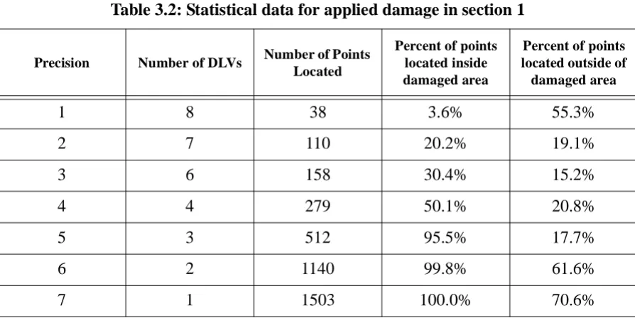
3.1 Number of DLVs for each precision for damage in section 1 . . . 263.2 Statistical data for applied damage in section 1 . . . 38
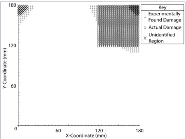
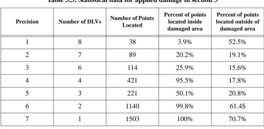
3.3 Statistical data for applied damage in section 3 . . . 40
3.4 Statistical data for applied damage in section 7 . . . 41
3.5 Statistical data for applied damage in section 5 . . . 42
3.6 Statistical data for applied damage in section 1 and 2 . . . 45
3.7 Number of points located for severity of damage in section 1 . . . 48
3.8 Number of DLVs for each section in the thirty-two sensor plate model . . . 53
3.9 Statistical data for applied damages in sections 1 through 10 . . . 60
4
Experimental Work
4.1 Properties for sensors in experimental setup from Equation 4.2 . . . 78Chapter 1
Introduction
The ability to detect damage in a structure while the structure is in service is important to many disciplines. When performed throughout its lifetime, this field is typically called structural health monitoring (SHM). SHM has applications in the civil, mechanical, and aerospace engineering fields amongst others. As structures become more complicated and the use of composite materials are more prevalent, the ability to detect and identify damage has also become increasingly more difficult. Many methods exist to replace visual inspection of the structure [1]. Visual inspections are a non-destructive approach to detect damage rather than a monitoring technique which implies some sort of automation. In order to increase the safety and decrease maintenance costs integrated sensors systems are being developed for the purpose of detecting damage before small controllable failures become catastrophic ones.
The current thesis presents a method that can localize damage in a structure using integrated displacement sensors. The method is a comparison method between undamaged and damaged states and is based on the flexibility response of both. The primary advantage of the method is that all required information is obtained from sensor and actuator data only. The sensors measure local displacements which are applied directly to the algorithm to locate the damage. There is no intermediate step that involves modelling. This is important because there is no error added from the intermediate step therefore the only error comes from the sensor and actuator data.
Chapter 2
Background
Background information covering several topics is presented in this chapter. Explained first are types of damages that occur in composites. Second, scales of detecting damage in a structure are outlined. Next, three different methods of identifying damage from the current literature are presented. Afterwards, work done by Bernal on a comparison based localization method is summarized. The work done by Bernal is the basis of the work presented in this thesis and subsequently the following section covers the governing equations of this research. Then, using these concepts, a five bar truss structure is used to show the usefulness of the current method. Finally, a review of fiber optic waveguides and fiber optic sensors are presented.
2.1 Damage identification
There are many ways to sense and assess damage in a structure but they can generally be placed into three categories of SHM: detection, localization and identification. Detection consists of knowing when the structure has been damaged. This is lowest level of monitoring because the system informs the user that damage has occurred. The next level is localization. Localization assists users by indicating where the damage has occurred which can decrease inspection times. Localization has many applications in the aerospace industry due to the intensive inspections currently being performed visually [1]. Finally, there is the final level of identification, which indicates to the user what specific type of damage has occurred. For example, in a composite this level would be able to differentiate between the above five damages. The work presented in this thesis is at the localization level. The approach will allow an user to minimize the area in a structure for inspection by indicating in what section damage has occurred.
2.2 Current damage detection methods
The field of SHM is not relatively new. Many research efforts have been focused on determining ways to detect, locate and identify damage in a structure. A driving force behind these efforts is to decrease maintenance costs [1]. In the following sections a few of the methods currently being researched are presented. Each method has specific applications in SHM and offers an insight into the different approaches to SHM. In addition, they will be used as comparisons for the method presented in this thesis. The following review is an overview of a few methods and is not a complete survey.
2.2.1 Frequency response methods
A widely applied method for detecting damage in structures is based on the
shapes, and modal dampings. Damages may induce coupling between vibration modes and it is these coupling effects that are used to locate damage. Lee and Shin present a method to reduce the equations of motion and therefore locate damage in a more efficient manner. The laboratory results of Lee and Shin are promising, however its application to real structures is uncertain because specific frequencies are needed in order to generate accurate information.
2.2.2 Model comparison methods
Another common method for detecting damage is through the comparison of a measured structural response with a pre-existing structural model (e.g. a finite element model). Seydel and Chang use this method to locate impact damage on stiffened panels by measuring strains determined by piezo ceramic sensors[4]. A problem seen in this work and many other model based techniques is the difficulty of sufficiently matching the model with the actual structure. Seydel and Chang showed that by using different boundary conditions in the structural model, better results could be produced [4][5]. For their example the actual plate was clamped at one end and simply supported at the other end. They applied two boundary conditions to the model, one with simply supported ends and the second with the boundary conditions found on the experimental plate. Their results showed that the simply supported ends located damage better then the actual boundary conditions of the plate [5]. Another problem that arises with this approach is the extensive computer resources required due to the complexity of the models. Therefore it is difficult to use such an approach for a real-time damage detection system.
2.2.3 Neural Networks
plate in order to obtain delamination location and size. They used a number specimens to train a neural network in order to locate damage on a specimen that was not trained. The use of neural networks improved their results. A similar approach was applied by Studer and Peters[7]. They detected the size, location and angle of a crack in a plate using strain and strain gradients for a specific sensor mesh. The neural network was first trained with known inputs of the strain and strain gradients values correlated to test crack parameters. The neural network was shown to improve the identification of the crack properties significantly as compared to a more classical approach. Unfortunately to achieve these advantages large training sets are typically developed through a structural model.
2.3 Flexibility approach to damage localization
The flexibility approach to damage localization, first presented by Bernal [8], is presented in the following section. This method will be used as the starting point for the research presented in this thesis. The flexibility method treats sensor data without the need to use an independent structural model. This means that the approach does not introduce
modelling error. The method is also able to locate single or multiple damages occurring simultaneously.
Ω
DU
Ω
Ω
DDLV DLV
DLV
When applying the flexibility method, the system must be treated as linear in the pre -and post- damage states. This assumption will restrict the types of damage that can be located with this technique, however it is still applicable for most foreseen damage occurrences. Next, assume there are a set of load vectors defined in sensor coordinates, which produce identical deformations at the sensors in the undamaged and damaged states [8]. These load vectors are referred to as damage location vectors (DLVs). Bernal derived the following equation for damage localization [8],
2.1
where, is the flexibility matrix of the damaged structure, and is the flexibility matrix of the undamaged structure. There are two possible solutions to Equation 2.1. The first is that
is equal to zero which means and are equal which implies no damage has occurred. The second is that L is the basis of null space of . Once L has been calculated from Equation 2.1, each of the base vectors are applied to the structure leading to zero stress in the damaged elements. Therefore the intersection of the zero stress regions corresponding to the stress distributions defined by each of the basis vectors of null space of can then be used to localize damage.
Bernal demonstrated his approach on a forty-four bar truss structure with ten sensors mounted to locate damage. He derived the flexibility matrices for damage localization by exciting the structure using white noise and measuring displacements in the vertical direction. Damage was introduced into the model by reducing the Young’s modulus of a bar. The technique was able to locate single and multiple damages each time. In a following article, Bernal considered damage localization of a plate [9]. Again damage was simulated by reducing the Young’s modulus for a region in the plate. Since the plate model was not
composed of discrete elements, the damage appeared as low stress regions due to the applied DLVs, rather than zero stress regions. These results indicate that the flexibility approach shows promising detection capabilities.
∆F L⋅ = 0
∆F = FD–FU
FD FU
∆F FD FU
∆F
2.4 Application of displacement sensors to the flexibility
approach
The goal of this work is to apply the principals of the flexibility approach, however replacing the vibration measurements with more reliable displacement measurements. It can be seen in both of Bernal’s works [8] [9], that specific frequencies are needed to generate data to locate damage. The ability to apply local forces has only recently been possible for a real structure due to the maturity of actuators such as SMAs and piezo ceramics. With the use of applied forces one is able to generate data that does not need specific inputs to produce good results. For N sensors located on a structure, we can define flexibility matrix , where is the applied force matrix and is the displacement matrix.
2.2 All matrices are defined in sensor coordinates. The flexibility matrix has dimensions N x N where N is the number of degrees of freedom. Solving Equation 2.2, one is able to find displacements in a structure for known applied loads or in the inverse case using the stiffness equation,
2.3 where is the structure stiffness matrix. Applying an appropriate set of displacements allows the flexibility matrix to be calculated directly by,
2.4 However, with certain boundary conditions of a structure, it is not always possible to experimentally generate an independent set of vectors to form , i.e. to derive a matrix that can be inverted. Instead, calculating the system stiffness, , by applying an appropriate applied force matrix and solving,
2.5 is often more feasible. Then the flexibility matrix is calculated via,
F [ ] [ ]α δ [ ] F [ ] α⋅[ ] = [ ]δ K [ ] δ⋅[ ] = [ ]α K [ ] F
[ ] [ ] αδ ⋅[ ]–1 = δ [ ] [ ]δ K [ ] α [ ] K
2.6 The stiffness matrix may be singular, however, due to the presence of rigid body motions in the system and therefore cannot be inverted to calculate . To eliminate this problem we define the free-free flexibility matrix,
2.7 which eliminates the effects of the rigid body motion [10]. In Equation 2.7, is the matrix constructed from the orthonormalized rigid body motions and is the projector matrix associated with the rigid body motions and defined by,
2.8 where is the identity matrix. The free-free flexibility matrix holds the same properties as the normal flexibility matrix, i.e. it is symmetric and orthogonal to all rigid body motions. The free-free flexibility matrix will be used in the following example.
2.5 Truss example
This section shows how DLVs are used to locate damage in a truss structure applying the technique described is the previous section. The truss structure used is a simple five bar, statically indeterminate truss, as seen in Figure 2.2. Sensors are placed at each node of the truss structure in each of the local coordinate directions. The numbering of the sensors is presented in Figure 2.3. All odd numbered sensors measure displacement in the x-direction
F
[ ] = [ ]K –1
F
[ ]
F
[ ] = [ ]P ([ ]K +[ ]R [ ]R T)–1
R
[ ]
P
[ ]
P
[ ] = [ ]I –[ ]R [ ]R T
I
and all even numbered sensors measure displacement in y-direction. The truss has properties shown in Table 2.1.
For this truss structure the force matrix was singular, therefore applying Equation 2.4 directly is not possible. Therefore, Equation 2.5 was used to calculate the stiffness matrix. The procedure used was to load the truss structure with eight independent loads and measure the subsequent displacements. For this truss structure, forces of 1 Newton (N) were applied at nodes 2 and 3 in each direction, giving a total of four loading conditions. Then the boundary conditions on nodes 1 and 4 were moved to nodes 2 and 3. Afterwards, forces on nodes 1 and 4 were applied in both directions yielding four more loading conditions. Since the truss is an eight degree of freedom system, a total of eight loading conditions are needed. Once all the data was gathered the stiffness (K) was calculated in the undamaged state.
As stated before this is a situation where the stiffness is not invertible due to the fact that the nodes were located at the boundary, therefore, they were restrained from displacing for some loading conditions. Therefore, the free-free flexibility equation was used (Equation 2.7 and Equation 2.8) where is,
Table 2.1: Truss properties
L 1 m
E 210 GPa
A 1 m2
L L Y X 3 2 1 5 4 1 2 3 4 q1 q2 q7 q8 q6 q5 q4 q3
1 Bar Number 1 Node Number q5 Local Coordinates
X Global Coordinates KEY
Sensors 3 & 4
Sensors 7 & 8 Sensors
5 & 6
Sensors 1 & 2
Figure 2.2: Geometry and symbols of the five bar truss structure.
Figure 2.3: Displacement sensor location of the five-bar truss.
R
2.9
Each of the columns of Equation 2.9 is associated with a specific rigid body motion. Column one represents translation in the x-direction, column two represents translation in y-direction and column three represents rotation about the center of the structure.
The next step is to apply damage to one of the bars to test the ability of the method to locate the damage. Two cases were considered. In the first case, the Young’s modulus of bar three was reduced by 25% and in the second simulation the Young’s modulus of bars two and five was reduced by 1% and 50% respectively. Once the damage has been simulated the next step is to calculate the damaged flexibility matrices which was done using the same procedure described above.
The next step is to find the null space of for the solution of the DLVs. For the simulation of damage in bar three the following DLVs were obtained,
2.10
Once the DLVs are determined, they are reapplied to the undamaged flexibility matrix as loads to the structure. From this, the displacements at each node were determined and the axial stress in each bar found through,
2.11
R
[ ] 1
8
---2 0 –1 0 2 1
2 0 1 0 2 1 2 0 –1 0 2 –1 2 0 –1 0 2 –1 =
FD–FU
L
0 1 0 0 –1 0 1 0 0 0 0 0 0 1 0 0 0 0 0 1 0 0 0 0 0 1 0 0 0 0 0 1 0 0 0 0 0 1 0 0 0 0 0 1 0 0 0 0 0 1 0 0 0 0 0 0 =
σ E ∆L
L
---⋅
The application of the DLVs generates an i x j matrix where i is the row number associated with each bar and j is the DLV number. The final results for this simulation are,
2.12
It can be seen that row three is the only row with all zero stresses. Therefore, taking the intersection of zero stress components in all the columns yields only the location of bar three. This identifies locations that are low stress regions with respect to ANY applied vector in the null space of . Now we repeat the calculations for the case of damage in bars two and five. The same procedure was performed for this simulation producing a final result of,
2.13
Again rows two and five are the only rows with all zero stress components in all columns. It can be seen that in both cases the damage was well located by this approach. In addition, the technique located multiple damages. As seen by the second example, it was able locate very small and large damages however was not able to distinguish between them. This confirms that the technique is a localization method. Once the damage has been located, it can be assessed by some other means depending on the particular application.
σAxial 1 4 2 ---– 1 2 2 --- 1 4 2 ---– 1 4 2 ---– 1 2 --- 1 4 2 ---– 1 2 2 ---– 1 4 2 --- 1 2 2 ---– 1 4 2 --- 1 4 2 --- 1 2 --- 1 4 2 --- 3 2 2 ---–
0 0 0 0 0 0 0
0 0 0 1
2 --- 1 2 ---– 1 2 ---– 1 2 ---1 2
---– 0 1
2
--- 0 1 2
---– 0 1
2 ---=
∆F
σAxial
2 0 2 0 0 0 0 0 0 0 0 0 5
2 --- 1 7
2 ---– 1
2 ---– 1 1
2 ---– 1
2 --- 0 1
2 ---– 1
2 --- 0 1
2.6 Fiber optic waveguides
Fiber optic waveguides were initially developed for telecommunications, but first appeared as a structural sensor by Butters and Hocker in 1978 [12]. Since then they have evolved into useful sensors. There are many ways to use a fiber optic waveguide as a sensor through taking advantage of its properties. In this section, the propagation of light through the fiber optic waveguide is discussed in order to show how it can be modified to measure strain. In addition, the theory of the fiber Bragg grating (FBG) sensor for the measurement of strain is discussed.
2.6.1 Introduction to fiber optic waveguides
Most optical fibers are made from silica. The fiber can be divided into three parts. The first part is the core. The core has a diameter of 9µm. Surrounding the core, is the cladding which has a diameter of 125µm. Both of these two parts are made of the same original silica. A fiber optic waveguide propagates light according to Snells Law of Refraction [13]. In a fiber optic waveguide the light is contained in the core by reflecting off the intersection of the core and cladding. In order to have complete internal reflection at the intersection of the core and the cladding, the index of refraction (n) of the core must be greater than that of the cladding. A typical optical fiber core has an index of refraction of around 1.46 while the cladding’s index of refraction is roughly 0.1% lower than the core’s index of refraction (Figure 2.5).
Index of Refraction
n2 n1 n2 Coating
Cladding
Core
Although the core is originally the same material as the cladding, its index of refraction is increased by doping with Germanium [13]. The process does not change the mechanical properties of the glass therefore for strain measurements, the core and cladding are considered the same material.
The final part of the optical fiber is the coating. This is strictly a protective part of the fiber. It is used to strengthen the fiber and protect it from moisture. The glass fiber is strong in tension but does not fair as well in bending. With the addition of the coating, the ability of the fiber to withstand bending increases. There are two types of coating common to optical fibers. They are polyimide and acrylate. Acrylate is generally used for telecommunications purposes while polyimide is primarily used in sensing applications. The properties of each can be seen in Table 2.2.
2.6.2 Advantages of fiber optic sensors
There are many different methods to use optical fibers as sensors and many different measurands that can be monitored by these. Strain, pressure, acceleration, rotation, and humidity are common examples. The reason why they have excelled in sensing is they have
Table 2.2: Fiber optic coating properties [13]
Coating
Outer Diameter
(µm)
Elastic Modulus
(MPa)
Tensile Strength
(MPa)
Static Fatigue Resistance
Minimum Temp. (C)
Maximum Temp. (C)
Acrylate 250 700 26 no 100 - 40
Polyimide 150 2400 130 yes 300 - 190
Input Light
Output Light
Core
Cladding
n = 1.45
n = 1.44
very good properties for that application. The first reason a fiber optic is a good sensor, is that it does not require a lot of wires. Unlike conventional electrical strain gages, a fiber optic waveguide has only one “wire” that both transmits information from the sensor and supplies the power. This can be seen in Figure 2.6. The information and power for three fiber optic sensors is transmitted through one fiber but nine wires are required for three electrical strain gages. Another advantage of fiber optic sensors are the ability to multiplex sensors. This means one optical fiber is able to contain numerous sensors without separate interrogation systems for each one. As seen in Figure 2.6, this fiber contains three sensors. Another advantage of a fiber optic waveguide is its ability to measure multiple measurands within a single fiber [14]. For example, a fiber optic sensor can measure strain, strain gradient,
integrated strain, and displacements. The ability to have different types of measures allows the user to learn more about the structure. The particular fiber optic sensor used in this work is based on a displacement sensor.
Fiber optic sensors can be used in many environments and locations which gives them a significant advantage over more conventional sensors. Since most fiber optic sensors are relatively small they can be embedded into composite materials [13]. The fiber form is very unobtrusive (Table 2.2) when it comes to embedding in fiber-reinforced composites, therefore they do not degrade the overall strength of the composite [15]. An optical fiber can withstand very high and low levels of heat depending on the coating. In addition to harsh temperatures, fiber optic sensors can be used in other hostile environments. Since no electrical current passes through the fiber they can also be used for two applications. The first is near highly sensitive equipment to electrical noise because a fiber optic sensors uses only light for
2.6.3 Fiber Bragg grating strain sensor
There are many types of sensors based on optical fibers. They can be made into several types of interferometers, for example, but the particular sensor used in this work is called a fiber Bragg grating (FBG). A FBG is a periodic modulation in the index of refraction along the axis of the core of the fiber [13]. There are several ways to induce this change in index of refraction of the core but the most common is by focusing an excimer laser through a phase mask onto the core of the fiber. This changes the index of refraction at the core but not the other properties of the optical fiber. The diffraction pattern caused by the phase mask writes a filter in the fiber. A schematic of a FBG can be seen in Figure 2.7. In addition, a phase mask setup can be seen in Figure 2.8.
Fiber Optic FBG
Electrical Strain Gage
Wires
As stated previously, a FBG acts as a filter for light. As light propagates through the fiber certain wavelengths are reflected while others are transmitted. As shown in Figure 2.9, if a broad spectrum of light is sent into the fiber, the result is two spectra. The transmitted
Input Light
Output Light Cladding
Sensor Core
Bragg Grating
Figure 2.7: Fiber Bragg grating showing schematically the periodic change in the index of refraction.
Phase Mask Cylindrical Lens
Rotatable and Laterally translatable
mirrors
Optical Fiber Zero
-order block Laser Source
spectrum is the same spectrum of the light entering the fiber but with some wavelengths of the grating filtered out. The reflected spectrum contains these filtered wavelengths.
Before a load is applied to the FBG, we have the original spectrum shown Figure 2.10. The wavelength at which the maximum amount of light is reflected is called the Bragg wavelength, λband can be seen in Figure 2.10. After an axial load is applied the spectrum shifts either to the right or left. Figures 2.11 and 2.12 show the peak shifts for axial loading in compression and tension. After this happens, a new maximum wavelength occurs,λf.
Reflec
tivit
y (%)
Wavelength (nm)
Reflec
tivit
y (%)
Wavelength (nm)
Reflec
tivit
y (%)
Wavelength (nm) Laser Light in
the Fiber
Reflective Spectrum From the Grating
Transmitted Spectrum From the Grating
Path of Travel of Laser Light
Key
Figure 2.9: Propagation of light waves through an optical fiber with a FBG.
λb Wavelength (nm)
Reflec
tivit
y (%)
After measuring the spectra for a FBG before and after loading has been applied, the applied axial strain value can be found using the following equation,
2.14
Equation 2.14 shows the linear relationship between applied strain and the shift in Bragg wavelength. The term is a material property of glass and is found experimentally. For the FBGs used in this thesis . In general the Bragg wavelengths used in the experimental work for this thesis have aλbof approximately 1550 nm. In this work the FBGs are used as displacement sensors as will be explained more in Chapter 4.
λb Wavelength (nm)
Reflec
tivit
y (%)
λf
Original Spectrum Spectrum with a Compressive Load
Key
λb
Wavelength (nm)
Reflec
tivit
y (%)
λf
Original Spectrum Spectrum with a Tensile Load
Key
Figure 2.11: FBG spectrum after compressive load has been applied.
Figure 2.12: FBG spectrum after tensile load has been applied.
ε 1
1–PE
( )
--- λf–λb
λb
---
=
PE
Chapter 3
Simulations
Whereas the truss was a simple tool for explaining the ability of the method to locate damage, an application that presents more interesting behaviors is a plate. For this chapter, a plate was modeled using ANSYS in order to demonstrate the ability of the method to locate damage. ANSYS is used to simulate sensor data that would normally be found
experimentally. It is not to be confused with using a structural model. The first case
considered is a plate that contains eight displacement sensors. Afterwards, a plate with thirty-two sensors is presented. As compared to the eight sensor plate, the thirty-thirty-two sensor plate has nine potential damage locations located internal to eight sensors. A new method is also developed where only the DLVs are used to locate damage to reduce the computation time required making the technique more suitable for real-time SHM systems. Through these simulations the flexibility method shows good potential for damage localization.
3.1 Eight sensor plate model
3.1.1 Model explanation
For this plate model, the eight sensors are placed in pairs. The sensor locations can be seen in Figure 3.2. The sensors are placed in the x-direction (odd numbers) and y-direction (even numbers). The sensors are assumed to measure displacements at a point at their location on the plate. The sensors were mounted in the center region of the plate to avoid edge effects and maximize sensitivity to damage.
180 mm
180 mm
X Y
Figure 3.1: Dimensions and boundary conditions for the eight sensor plate model.
180 mm
180 mm
60 mm
60 mm 60 mm
60 mm
1 6 4
3 5
2 8
7
4 Sensor Number Key
3.1.2 Calculation of a flexibility matrix
To meet the goal of developing the plate’s flexibility matrix without structural modeling, a procedure was developed to obtain the flexibility from only sensor and actuator data. The procedure consists of applying a point force at each sensor location in the direction of the sensors. A unit force (1 N) was applied one at a time at each sensor location and the displacements at each location were recorded. From these displacements the undamaged flexibility matrix for the plate was built, . Since unit loads were applied the flexibility matrix could be constructed directly from the data as follows,
3.1
3.2
3.3 To illustrate how the procedure operates, Figures 3.3 and 3.4 display each step in the creation of the flexibility matrix. The (i, j) component of the flexibility matrix corresponds to the displacement of the ithsensor due to the unit load applied at the jthsensor. In addition it can be seen in the figures that the flexibility matrix is also symmetric as mentioned in the
background.
3.1.3 Damage localization
For the purpose of inducing damage, the plate was divided into the nine regions shown in Figure 3.5. In order to simulate damage of a particular section of the plate its Young’s modulus was reduced to 0.15 GPa. No other properties were changed. Once damage had been induced, the same procedure for obtaining the flexibility matrix, , was performed. For the eight sensor plate model, five areas of damage were simulated. These damages occurred in sections 1, 3, 5 and 7. A final damage was simulated, located partially in sections 1 and 2 with dimensions of 60 mm by 60 mm.
FU
FU
[ ] [ ] αδ ⋅[ ]–1 =
α
[ ] = [ ]I 8×8 = [ ]α –1
FU
[ ]= [ ]δ ∴
0.0007594386780 0.000027844824 0.000443451680 0 0 0 0 0 0.000027844824 0.000550563432 0.000076738476 0 0 0 0 0 0.000443451680 0.000076738476 0.0014400122680 0 0 0 0 0 0.000051133295 0.000161068093 0.0001369552460 0 0 0 0 0 0.0004308211840 0.0000873097170 0.0009628782510 0 0 0 0 0 0.0000702675890 - 0.0001146820820 0 0 0 0 0 0.0002909210360 0.000012709193 0.0004308211840 0 0 0 0 0 - 0.000012709193 0.000044199970 - 0.0000873097170 0 0 0 0 0
- 4.763603 E-6
0.0007594386780 0 0 0 0 0 0 0 0.000027844824 0 0 0 0 0 0 0 0.000443451680 0 0 0 0 0 0 0 0.000051133295 0 0 0 0 0 0 0 0.0004308211840 0 0 0 0 0 0 0 0 0 0 0 0 0 0 0.0002909210360 0 0 0 0 0 0 0
−0.000012709193 0 0 0 0 0 0 0 - 4.763603 E-6
0.0007594386780 0.000027844824 0.000443451680 0.000051133295 0 0 0 0 0.000027844824 0.000550563432 0.000076738476 0.000161068093 0 0 0 0 0.000443451680 0.000076738476 0.0014400122680 0.0001369552460 0 0 0 0 0.000051133295 0.000161068093 0.0001369552460 0.000718629326 0 0 0 0 0.0004308211840 0.0000873097170 0.0009628782510 0.0001146820820 0 0 0 0 0.0000702675890 - 0.0001146820820 0.000125376006 0 0 0 0 0.0002909210360 0.000012709193 0.0004308211840 0 0 0 0 - 0.000012709193 0.000044199970 - 0.0000873097170 0.0000702675890 0 0 0 0
- 4.763603 E-6
4.763603 E-6 0.0007594386780 0.000027844824 0 0 0 0 0 0
0.000027844824 0.000550563432 0 0 0 0 0 0 0.000443451680 0.000076738476 0 0 0 0 0 0 0.000051133295 0.000161068093 0 0 0 0 0 0 0.0004308211840 0.0000873097170 0 0 0 0 0 0 0.0000702675890 0 0 0 0 0 0 0.0002909210360 0.000012709193 0 0 0 0 0 0 - 0.000012709193 0.000044199970 0 0 0 0 0 0
- 4.763603 E-6 X Y
F = 1 N
X Y
F = 1 N
X Y
F = 1 N
X Y
F = 1 N
mm N mm N mm N mm N
- 4.763603 E-6
0.0007594386780 0.000027844824 0.000443451680 0.000051133295 0.0004308211840 0.0002909210360 - 0.000012709193 0.000027844824 0.000550563432 0.000076738476 0.000161068093 0.0000873097170 0.0000702675890 0.000012709193 0.000044199970 0.000443451680 0.000076738476 0.0014400122680 0.0001369552460 0.0009628782510 - 0.0001146820820 0.0004308211840 - 0.0000873097170 0.000051133295 0.000161068093 0.0001369552460 0.000718629326 0.0001146820820 0.000125376006 0.0000702675890 0.0004308211840 0.0000873097170 0.0009628782510 0.0001146820820 0.0014400122680 - 0.0001369552460 0.000443451680 - 0.000076738476 - 4.763603 E-6 0.0000702675890 - 0.0001146820820 0.000125376006 - 0.0001369552460 0.000718629326 0.000051133295- 0.000161068093 0.0002909210360 0.000012709193 0.0004308211840 0.000443451680 - 0.000051133295 0.0007594386780 - 0.000027844824 - 0.000012709193 0.000044199970 - 0.0000873097170 0.0000702675890 - 0.000076738476 0.000161068093 0.000027844824- 0.000550563432
4.763603 E-6
4.763603 E-6 - 4.763603 E-6
4.763603 E-6
0.0007594386780 0.000027844824 0.000443451680 0.000051133295 0.0004308211840 0.0002909210360 0 0.000027844824 0.000550563432 0.000076738476 0.000161068093 0.0000873097170 0.0000702675890 0.000012709193 0 0.000443451680 0.000076738476 0.0014400122680 0.0001369552460 0.0009628782510 - 0.0001146820820 0.0004308211840 0 0.000051133295 0.000161068093 0.0001369552460 0.000718629326 0.0001146820820 0.000125376006 0 0.0004308211840 0.0000873097170 0.0009628782510 0.0001146820820 0.0014400122680 - 0.0001369552460 0.000443451680 0 0.0000702675890 - 0.0001146820820 0.000125376006 - 0.0001369552460 0.000718629326 0.000051133295 0 -0.0002909210360 0.000012709193 0.0004308211840 0.000443451680 - 0.000051133295 0.0007594386780 0 - 0.000012709193 0.000044199970 - 0.0000873097170 0.0000702675890 - 0.000076738476 0.000161068093 0.000027844824 0
-- 4.763603 E--6
4.763603 E-6 0.0007594386780 0.000027844824 0.000443451680 0.000051133295 0.0004308211840 0 0
0.000027844824 0.000550563432 0.000076738476 0.000161068093 0.0000873097170 0.0000702675890 0 0 0.000443451680 0.000076738476 0.0014400122680 0.0001369552460 0.0009628782510 - 0.0001146820820 0 0 0.000051133295 0.000161068093 0.0001369552460 0.000718629326 0.0001146820820 0.000125376006 0 0 0.0004308211840 0.0000873097170 0.0009628782510 0.0001146820820 0.0014400122680 - 0.0001369552460 0 0 0.0000702675890 - 0.0001146820820 0.000125376006 - 0.0001369552460 0.000718629326 0 0 0.0002909210360 0.000012709193 0.0004308211840 0.000443451680 - 0.000051133295 0 0 - 0.000012709193 0.000044199970 - 0.0000873097170 0.0000702675890 - 0.000076738476 0.000161068093 0 0
- 4.763603 E-6
- 4.763603 E-6
4.763603 E-6
0.0007594386780 0.000027844824 0.000443451680 0.000051133295 0.0004308211840 0 0 0 0.000027844824 0.000550563432 0.000076738476 0.000161068093 0.0000873097170 0 0 0 0.000443451680 0.000076738476 0.0014400122680 0.0001369552460 0.0009628782510 0 0 0 0.000051133295 0.000161068093 0.0001369552460 0.000718629326 0.0001146820820 0 0 0 0.0004308211840 0.0000873097170 0.0009628782510 0.0001146820820 0.0014400122680 0 0 0 0.0000702675890 - 0.0001146820820 0.000125376006 - 0.0001369552460 0 0 0 0.0002909210360 0.000012709193 0.0004308211840 0.000443451680 0 0 0 - 0.000012709193 0.000044199970 - 0.0000873097170 0.0000702675890 - 0.000076738476 0 0 0
- 4.763603 E-6
4.763603 E-6 X
Y
F = 1 N
X Y
F = 1 N
X Y
F =1 N
X Y F = 1 N
For each damage that was simulated, a new matrix was created. Once the damage matrices had been found for each damage, the next step was to determine through
Equation 2.1. The next step was to find the null space of in order to obtain the DLVs. Once the DLVs were calculated, they were reapplied to the structure in order to determine the zero stress areas. This procedure is the same as for the truss, as described in Chapter 2. Since the plate has several differences as compared to the truss and there are many steps involved in locating damage, the process will be explained for damage in section 1 only. The reason the plate is different is because it is not an exact solution due to the FE approximation.
The calculation of the null space L for Equation 2.1 were performed in Mathematica using the command line found in Equation 3.4.
3.4 In order to determine the null space of using this or any other solver, the precision of the components of must be specified. Precision in Mathematica is defined by the number of significant digits in a value. Since the results of damage localization depend on the precision used (i.e. the size of the null space changes), a procedure was developed to find the range of precisions for which the Mathematica solver generated a null space for each simulated damage. For section 1 the highest precision obtained was seven and the lowest was one. Once the allowable precisions were determined, the null space was calculated to obtain the DLVs.
FD
∆F
∆F
60 mm
60 mm
60 mm
60 mm 60 mm 60 mm
1
2
3
4
5
6
7
8
9
Sensor Locations Key
Figure 3.5: The nine damage sections of the eight sensor plate model.
DLV = NullSpace[∆F Precision, ]
∆F
The number of DLVs obtained from each precision value are listed in Table 3.1 and their values are given in Figure 3.6 for damage in section 1.
It can be seen that as the precision is increased, the number of DLVs decreases for a given damage. This is to be expected since the null space of a matrix increases as the number significant digits in the terms decrease. Here one also notes that in most sets of DLVs, the lowest values in magnitude are typically located at the sensors closest to the damage. For the example of damage in section 1, the sensors that are closest to the imposed damage are sensors three and four. Looking at rows three and four in Figure 3.6, for all precision values, it is evident that these are consistently the lowest values. This feature will be exploited later.
The next step in the damage localization procedure is to reapply each DLV to the undamaged plate model in ANSYS separately to calculate the in-plane stresses at each node,
σx,σyandσxy. This is shown schematically in Figure 3.7 for one of the DLV sets.
Table 3.1: Number of DLVs for each precision for damage in section 1
Precision Number of DLVs
7 1
6 2
5 3
4 4
3 6
2 7
![Figure 2.1: Schematic illustration of damaged and undamaged domains [8].](https://thumb-us.123doks.com/thumbv2/123dok_us/1317616.1164525/24.612.243.394.342.504/figure-schematic-illustration-damaged-and-undamaged-domains.webp)