Twitter Analytics: Geotag Imputation, Forecasting, and Dynamic Variable Selection.

(1)

ABSTRACT

BAKERMAN, JORDAN. Twitter Analytics: Geotag Imputation, Forecasting, and Dynamic Variable Selection. (Under the direction of Alyson Wilson.)

The popularity of social media has created vast repositories of open source data with broad potential value. Researchers are actively mining these new complex data sources to create predictive models for wide-ranging applications. For example, Wikipedia is used to forecast influenza in the United States [Hickmann et al., 2015], Facebook is used for more effective advertising [Backstrom et al., 2010], and Twitter is used to forecast civil unrest in Latin America [Korkmaz et al., 2015]. In this dissertation, we create statistical methodology advancing the analytical value of Twitter.

We begin in Chapter 2 by developing a geotag imputation method to predict the origin of individual tweets. Standard practice uses either the content of the tweet, network in-formation, or these two features independently to estimate the origin. We show improved accuracy by using both tweet text and user network information jointly. Moreover, we properly account for uncertainty, improving both precision and coverage of geotag impu-tation.

(2)

regions in order to contextualize the reasons for protest. The proposed methodology is scalable and outperforms the current baseline.

(3)

(4)

Twitter Analytics: Geotag Imputation, Forecasting, and Dynamic Variable Selection

by

Jordan Bakerman

A dissertation submitted to the Graduate Faculty of North Carolina State University

in partial fulfillment of the requirements for the Degree of

Doctor of Philosophy

Statistics

Raleigh, North Carolina

2018

APPROVED BY:

Eric Laber Donald Martin

John Mattingly Karl Pazdernik

External Member

Alyson Wilson

(5)

DEDICATION

(6)

BIOGRAPHY

(7)

ACKNOWLEDGEMENTS

(8)

LIST OF TABLES

Table 2.1 The simple accuracy error metric compared to the literature using the Eisenstein data set from 2010. Results are reported in kilometers using

the great-circle distance function. . . 25

Table 2.2 The comprehensive accuracy error, prediction region area, and coverage metrics compared to Priedhorsky et al. [2014] because both algorithms use Guassian mixture models. The weighting scheme applied by Pried-horsky et al. [2014] is the sum of the product of the elements in each covariance matrix of each GMM. . . 27

Table 3.1 Forecast results for structural break parameters and T “50. . . 67

Table 3.2 Forecast results for structural break parameters and T “100. . . 68

Table 3.3 Variable selection results for structural break parameters. . . 68

Table 3.4 Forecast results for completely dynamic parameters and T “50. . . . 69

Table 3.5 Forecast results for completely dynamic parameters and T “100. . . . 69

Table 3.6 Variable selection results for completely dynamic parameters. . . 70

Table 3.7 Civil unrest forecast results for each country, model, and forecast period. 76 Table 3.8 The top four most commonly selected variables for each country and model. . . 77

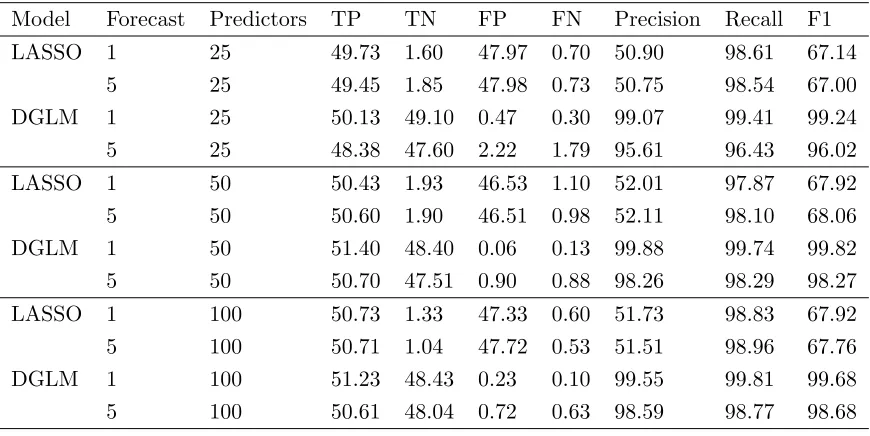
Table 4.1 Forecast results for time series length T “25. . . 102

Table 4.2 Forecast results for time series length T “50. . . 102

Table 4.3 Influenza forecast results for each region, model, and forecast period. . 108

(11)

LIST OF FIGURES

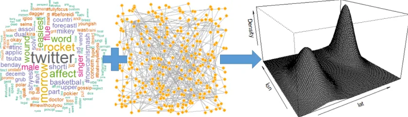
Figure 2.1 The general approach to our hybrid method. Combine Twitter text and network information to predict location with a bivariate density estimate. . . 11 Figure 2.2 A set of text or network coordinates. The‹‹‹observations are considered

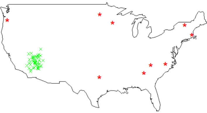
outliers and removed before the Gaussian Mixture Model is created. . 18 Figure 2.3 An example of the hybrid model density estimate, hpy|m, njq,

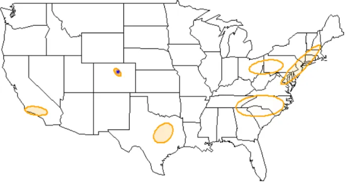
predict-ing location of a spredict-ingle tweet. Each ellipse models a separate subpopu-lation and the darker the transparency the higher the probability. The true origin of the tweet is marked by the ‹‹‹symbol. . . 22 Figure 2.4 Locations of all tweets within the Eisenstein data set. . . 24 Figure 2.5 Geographic probability distribution of influenza in the United States

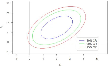
during March of 2010. . . 30 Figure 3.1 Example of the joint credible region variable selection approach for a

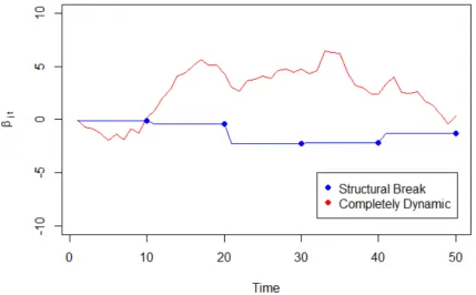
linear model with two parameters. Here the solution path is tβ1.β2u. . 59 Figure 3.2 Example of a single structural break and completely dynamic parameter. 63 Figure 3.3 The number of protest and non-protest days for Argentina, Brazil,

Colombia, Mexico, Paraguay, and Venezuela from November 2012 to August 2014 according the the Gold Standard Report. . . 72 Figure 3.4 Word cloud of the 962 term dictionary of protest related words, phrases,

and political leaders used to filter tweets and collect daily word counts. Terms are randomly scaled for the purpose of this graphic only. . . . 73 Figure 4.1 Locations of all 44,358 tweets sampled to train the hybrid geotag

im-putation model. . . 104 Figure 4.2 Weekly influenza-like illness (ILI) rates from October, 2016 to March,

(12)

Chapter 1 Introduction and Motivation

(13)

1.1 Geotag Imputation

Each tweet can be geotagged with a latitude and longitude pair, either according to a user’s cell phone geo-location service or the HTML5 geolocation API when a person tweets from their computer. However, Twitter users may remove this geotagging option, and most do so. A recent study of Twitter showed less than 1% of tweets are geotagged [Ajao et al., 2015]. Given that a majority of tweets do not contain an origin, and therefore potentially useful tweets are without geographic context, considerable research has been devoted to geotag imputation.

There are two approachs to geotag imputation in the Twitter literature. The first approach relies on mining the 1% of geotagged tweets to find spatially predictive terms. For example, the term “#WolfPackNation” is used to acknowledge North Carolina State University. To impute a geotag for a tweet that contains the term “#WolfPackNation”, given no other spatially meaningful terms, it is likely the term originated near Raleigh, North Carolina. The second approach estimates location using network analytics. Re-searchers construct network graphs of the user posting the message and then estimate the origin of the tweet according to where users in the network typically tweet. For ex-ample, if all of ones’ friends tweet from Washington, D.C., it is likely the user with an unknown origin also tweets from the nation’s capital.

(14)

weight each model feature by its predictive power, nor does it account for the uncertainty in the location estimate.

In Chapter 2 we develop a hybrid geotag imputation model which uses both text and network features jointly. Our model weights the features according to their geographic scope in order to estimate location using all information simultaneously. In addition, we extend the work of Priedhorsky et al. [2014] by also using Gaussian mixture models to map the spatial distribution of each feature. This allows us to account for uncertainty by estimating the most likely origin of the tweet using a bivariate probability distribution across the earth’s surface. By modeling features jointly we show a significant gain in accuracy compared to Rahimi et al. [2015] and improve on the precision and coverage metrics of Priedhorsky et al. [2014].

1.2 Forecasting and Dynamic Variable Selection

Twitter has become a powerful tool for predicting real world affairs. Researchers mine the user generated content and use daily word counts to forecast diverse outcomes. For example, terms like “flu” and “fever” are leading indicators of influenza like illness rates reported by the Centers for Disease Control and Prevention in the United States [Achrekar et al., 2012]. Similarly, daily word counts have been used to forecast stock price movement [Bollen et al., 2011], box office revenue for the film industry [Asur and Huberman, 2010], and inner city crime rates [Gerber, 2014]. The models used to forecast the aforementioned outcomes, and others, are predominantly static or use a simple autoregressive structure. For time series data, the static model does not account for correlated observations, and as a result, it ignores useful forecasting information.

(15)

countries Argentina, Brazil, Colombia, Mexico, Paraguay, and Venezuela. Moving away from static methodology, we adopt dynamic logistic regression to forecast the probability of future protest. Compared to the static logistic regression baseline approach, dynamic logistic regression accounts for dependencies in successive observations and therefore, is better suited for time series data. Furthermore, the intrinsic Bayesian structure of dynamic models allows parameters to be sequentially updated in time as new information becomes available. This allows forecasts to be heavily weighted towards new information and is the reason dynamic models excel in short term forecasting. We show the dynamic approach is highly advantageous as it heavily outperforms the baseline method in terms of forecast accuracy.

(16)

1.3 Measurement Error

Geotag imputation and forecasting events with Twitter are currently separate research areas in the literature. Practitioners have yet to utilize tweets with imputed geotags in forecasting models. For some analyses, such as forecasting stock market indicators [Zhang et al., 2011], researchers are able to use tweets without an origin as location is irrelevant for the problem. For geographic specific models, such as forecasting civil unrest in Latin America [Korkmaz et al., 2015], researchers could substantially increase the supply of data by using tweets with imputed geotags. As a result, researchers may be able to improve the location granularity of the forecast event from the country level to perhaps state or city level.

(17)

Chapter 2 Geotag Imputation: A Hybrid

Approach

2.1 Overview

(18)

2.2 Introduction

Twitter was created in 2006 as a free online social networking service. The service allows its users to post messages with a maximum 140 characters called “tweets” without restric-tion on the number of tweets sent in any given time period. As of 2015, Twitter generates more than 500 million tweets daily, representing in excess of 300 million active monthly users [Ajao et al., 2015]. The popularity of Twitter has spawned a variety of research efforts to use the micro-blogging service as a tool to support many applications, includ-ing event detection [Korkmaz et al., 2015], event monitorinclud-ing [Gelernter and Mushegian, 2011], and influenza diffusion [Generous et al., 2014]. Each of these applications benefits from location information to identify and utilize relevant tweets.

Each tweet can be geotagged with a latitude and longitude pair, either according to a user’s cell phone geo-location service or the HTML5 geolocation API when a person tweets from their computer. However, Twitter users may remove this geotagging option, and most users do so. A recent study of Twitter showed that less than 1% of tweets are geo-tagged [Ajao et al., 2015]. As a result, recent research has focused on estimating location information in the Twittersphere.

(19)

“follow” other members of the community and converse with people directly using the

@username syntax. It is through the follower and followee relationships or direct mes-saging that one can derive a Twitter user’s network and use it as a model feature. If a particular tweet is intended for a specific user, the tweet field contains the user name. This direct engagement in an online conversation can be considered the requirement for two users to be “friends” and to create individual friendship networks.

The language, location, and time zone fields can be highly inaccurate because users may set these fields without protocol. Some authors use these fields as model features or as a test of accuracy for the ground truth and other authors only include tweets for model training with a real location field that can be mapped using a gazetteer [Cheng et al., 2010; Schulz et al., 2013; Davis Jr et al., 2011; Abrol and Khan, 2010; Rout et al., 2013]. However, an “actual” location does not mean it is the user’s true location. Only 66% of users provide accurate location field information, and nearly all at the city or state level [Hecht et al., 2011].

The current state of the Twitter geotagging literature can be described according to the model features. One segment uses the tweet text only, and another uses network information only, but there is little overlap between the two methodologies. The first seg-ment mines the training set of tweets, which are tweets with true geotagged coordinates, to find n-grams with little geographic variability. In other words, these methods identify sets of co-occuring words that are geographically narrow and predictive of location. For example, the termCeltics is vernacular most used in the Boston area. The network seg-ment, on the other hand, uses the distribution of friends to predict location. This notion is predicated on the idea that Twitter relationships mimic off-line relationships [Rout et al., 2013].

(20)

have evolved to consider prediction accuracy as the metric for quality. Whether classifying a tweet into a predefined region or predicting the latitude ˆlongitude origin of a tweet,

current approaches can predict a tweet to within a few hundred kilometers. The literature is described more fully in Section 2.3.

In this chapter, we propose a hybrid method (Figure 2.1) that can harness the power of both text and network features. Our method proves to be highly competitive with the current state of the literature according to multiple metrics. We are able to pinpoint the origin of a tweet to within 19 km more than 50% of the time. In addition, our approach has several key advantages compared to the literature.

1. We use a hybrid model.We provide a method to incorporate both text and network information to obtain a more accurate location estimate. In addition, increasing the number of model features correlates to predicting a larger number of tweets. The hybrid approach can still be used if at least one of the features, text or network, is available. If a tweet does not contain any predictive text, the hybrid model will use the network information only, and vice versa.

2. The text and network features are used jointly as predictors. Our model weights the features according to their geographic scope. This contrasts to the only other hybrid model in the literature [Rahimi et al., 2015], which uses text and network features consecutively without regard for the predictive power of each feature.

3. We avoid using a gazetteer. Filtering training tweets by accurate location field information can highly reduce the training set size. We use all tweets (divided into training and test sets) tagged with a latitude ˆlongitude pair.

(21)

problem and not a classification problem. We avoid creating predefined geographic regions which are subject to data sparsity difficulties.

5. More complete preprocessing.We take several text mining preprocessing steps to clean the data. We also remove outliers for the text features that skew predictions.

6. We use Gaussian Mixture Models.

(a) GMMs are scalable. This modeling technique is computationally inexpensive and, as a result, scales to large data sets. It also allows for efficient testing of different component mixture models to find the best fitting model.

(b) GMMs are multi-modal. Model features must be geographically narrow to represent a good predictor, but a single prediction region is not necessary. Mul-tiple locations are estimated for a single tweet with associated probabilities to gauge each location’s possibility as the origin. For example, the wordBurlington

is linked to over 20 cities in the United States.

(c) GMMs are interpretable probability distributions. GMMs provide a nat-ural way to interpret results and model error. Location estimates are bivariate probability distributions, visually displaying the most likely origin of a tweet and the model confidence in the estimate.

(22)

Figure 2.1: The general approach to our hybrid method. Combine Twitter text and network information to predict location with a bivariate density estimate.

2.3 Related Work

The current geotagging literature can be grouped into three categories: text, network, and hybrid methods. We briefly describe the state of the literature for each category.

2.3.1 Text Approaches

In one of the first Twitter geotagging methods, Eisenstein et al. [2010] developed a latent variable model that treats the text and location of tweets as outputs from a generative process. The authors showed that lexical variation, and text in general, can be predictive of location. Furthermore, they created a freely available data set of nearly 380,000 tweets that we use for model comparison with the literature. The data set is described more fully in Section 2.6.

(23)

the frequency of words within regions to train a model and predict location using Bayes Theorem. For example, naive Bayes is a simple and scalable method used to estimate the probability of a categorical event, such as the city origin of a tweet. The highest probability event is then regarded as the classification estimate.

The more recent text-based approaches move away from classification techniques to predict the latitude and longitude coordinate pair. The authors in Schulz et al. [2013] use a method calledpolygon stacking to estimate unique geographic regions. The authors use words that can be mapped to a region according to a gazetteer, which is a geographical dictionary. Words with geographical meaning, such as “Okemo Mountain,” are mapped to a physical location representing a geographic polygon. Each polygon for each word in the tweet is then stacked on top of each other and the center of the tallest plateau is considered the location estimate.

In a more intuitive approach, Priedhorsky et al. [2014] use Gaussian mixture models to estimate geographic probability distributions. The authors show that the technique is scalable, multi-modal, geographically interpretable, and avoids artificial boundaries. For these reasons, the Gaussian mixture model is the basis of our new algorithm.

2.3.2 Network Approaches

(24)

friends, F1, . . . , Fn, and the locations of each ofF1, . . . , Fn’s friends as well. The authors

in Rout et al. [2013] use support vector machines to classify at the city level in the United Kingdom using features such as city population and the number of reciprocated tweets. In addition, Rout et al. [2013] scale the population density of each city to avoid weighting the model towards the largest city, i.e., London.

As with the text-based approaches, some methods focus on classification, while others try to predict location according to the latitude and longitude coordinate pair. Although not initially intended for Twitter, Backstrom et al. [2010] establishes one of the first geotagging methodologies for social media, specifically Facebook. The authors show em-pirically that the probability of friendship is inversely proportional to the geographic distance between two people and use these probabilities within a likelihood approach to estimate the most probable location of a user compared to the locations of a set of other users. The authors in McGee et al. [2013] extend this method to Twitter and use regression trees to first estimate the strength of friendship between users. The strength of friendship determines which probability curve is used within the likelihood.

(25)

label propagation and consider the frequency of directed tweets as edge weights.

2.3.3 Hybrid Approach

We are aware of only one hybrid geotagging approach, which uses both text and network structure. Rahimi et al. [2015] borrow techniques from the text and network approaches to form a hybrid model. First, the authors discretized the geographic space using the method detailed in Wing and Baldridge [2014]. Then, unigrams appearing in at least ten tweets are used as features to train a logistic regression model. The model is then used to predict the most likely cell for an unknown user and the center of the cell is the coordinate location estimate. Next, the authors use the spatial label propagation method proposed by Jurgens [2013]. This iteratively adjusts the estimates from the text method by using the geometric median of locations of a user’s friends to predict location.

(26)

2.4 Preprocessing

Prior to model creation, we filter the data extensively. These steps are designed to filter noise from Twitter data and allow discovery of relationships between the model features and the geographic coordinates.

2.4.1 Text Preprocessing

The four text preprocessing steps below, in combination, reduce the number of unigrams present in the data and increase the rate of sparse words. For example, the words cool

and COOOOL are considered the same unigram. Therefore, we obtain two instances of a single unigram instead of one instance of two separate unigrams. As a result, we are able to supply our subsequent analyses with more data. To illustrate the steps, consider the following tweet as an example.

Hey @kpazphd OMG! my new car is SWEEEET!!! #TESLAlife watch out Raleigh!

livin the dream...

(27)

hey @kpazphd omg my new car is sweeeet #teslalife watch out raleigh livin the dream

Next, we remove all stop words because we assume there is no association between the most common words used in Twitter and geographic location. Stop words are simply the most common words in a given language. For example the, is, and no are common English stop words. However, there is no universal set of stop words. We combine two dictionaries for this preprocessing step. We combine the SMART stop word list, a list of 571 words developed by Cornell [Feinerer et al., 2008], and also the top 500 most common Twitter words uncovered by TIME magazine [TIME, 2009]. The second list is used to remove common slang terms such as lol, omg, and wtf from the Twitter feed.

hey @kpazphd car sweeeet #teslalife watch raleigh livin dream

Next, we perform a spell check on the remaining words that do not start with the @ or # symbol. Thus, we assume the association between misspelled words and geographic location is the same as correctly spelled words and geographic location. Each remaining word is compared to an English dictionary for accuracy. If the word is misspelled, it is replaced with the closest matching word according to the Jaccard coefficient for strings. The Jaccard coefficient simply measures the similarity between two sets,|AXB|{|AYB|.

In the context of language processing,A and B are two separate unigrams for which the letters are compared.

hey @kpazphd car sweet #teslalife watch raleigh living dream

Finally, we apply the Porter stemming algorithm, a widely used English stemming algorithm [Porter, 1980]. This reduces each remaining word to its root. For example, the words jumping,jumper, and jumped are set to the root word jump.

(28)

2.4.2 Text and Network Preprocessing

The unigrams present after the preprocessing steps above are then used to create unigram variables. Each unigram variable simply represents the locations (in latitudeˆlongitude coordinates) from which it was tweeted.

Likewise, we create each user’s network by considering direct tweets the barometer for friendship. A directed tweet is equivalent to sending a message to a specific person in a public forum. Directed tweets are performed using the@username syntax to refer to a specific user. That is,userAsends a direct tweet touserB by simply including the syntax

@userB in the tweet. In one study, Huberman et al. [2008] shows that approximately 25% of posts are directed tweets. To createuserA’s network, we find every instance when

userA sends a direct tweet. The users receiving the direct tweet are considered userA’s friends. We then search for tweets inititated by these friends that are also geotagged and include them in the network. userA’s network variable is now associated with a set of coordinates (latitudeˆ longitude). This process is repeated for each user.

A final preprocessing step is applied to both the text and network variables. We cluster the data into subpopulations for outlier prepossessing using the well-known K-means clustering procedure. This algorithm clusters data into k clusters and finds their centers by minimizing the sum of Euclidean distances of all data points to their respective centers. To estimate the number of appropriate clusters for each variable, we use the Gap statistic [Tibshirani et al., 2001]. This technique chooses k by finding the largest discrepancy of the pooled within-cluster sum of squares, Wk, for the data and the expectation of Wk

under a null distribution,

argmax

kPt1,...,20u

(29)

For simplicity, we use a uniform distribution over the range of observed data for each variable.

If an observation is farther than the mean distance from the center of its subpopula-tion, it is considered an “outlier” and removed from the data set [Aggarwal and Singh, 2013]. For tightly clustered data this removes subpopulation anomalies. Figure 2.2 illus-trates this technique.

In addition, we remove all text variables with less than ten observations to avoid modeling sparse data in the next section. This final technique is widely adopted in the geotagging literature [Eisenstein et al., 2010; Wing and Baldridge, 2011; Hulden et al., 2015; Priedhorsky et al., 2014].

(30)

2.5 New Hybrid Model

Our hybrid model is constructed using a series of Gaussian mixture models. We first create a bivariate density estimate for each unigram ui and network nj. Here, i and j

represent the index for the unique unigrams and networks respectively. Then we com-bine the appropriate unigram and network Gaussian mixture models using an intuitive reweighting algorithm to create a final Gaussian mixture model,hp¨q. This final model is a geographic probability distribution representing an estimate of the origin location of a non-geotagged tweet. The rest of this section details the creation of hp¨q.

Let yPR2 be a single pair of coordinates, latitude ˆlongitude. For each unigram ui

we fit a Gaussian mixture model to the observed locations,

gpy|uiq “ ci

ÿ

k“1

φikNpy|µik,Σikq, (2.1)

where N is the bivariate normal density function with parameters µik and Σik as the

mean vector and covariance matrix respectively. In addition, φik are the mixture weights

which combine the subpopulation probability distributions into a single density estimate. The subscript k represents the individual mixture components for each GMM and ci is

the number of mixture components for unigramui. The parameters φik, µik, and Σik are

estimated using the expectation maximization algorithm from the MCLUST package in

R [Fraley et al., 2012]. The volume, shape, and orientation of each mixture are free to vary, which implies that all three covariance matrix parameters must be estimated.

The authors in Priedhorsky et al. [2014] use a simple heuristic approach to choose the number of components for each GMM, minp20,logpsq{2q, where s is the sample size.

Instead, we choose the number of components, ci, which yields the best Bayesian

(31)

arg min ci ˆ ´2 si ÿ

b“1 log

„ ci

ÿ

k“1 ˆ

φikNpyb|µˆik,Σˆikq



`plogpsiq

˙ .

Here, p represents the number of parameters to be estimated and si is the sample size.

We use the BIC to balance both model fit and model complexity. Similarly, define the Gaussian mixture model for a user’s network as

fpy|njq “ cj

ÿ

k“1

θjkNpy|µjk,Σjkq. (2.2)

The number of components,cj, as well as the parametersθjk, µjk, and Σjk are estimated

in the same fashion as before. Recall from Section 2.4 that the data used to fit each network GMM are the locations where users within the network tweeted. That is, the coordinates of the network are targets to fit the GMM and estimate parameters similarly to the unigram GMMs.

Next, we combine the applicable text and network GMMs above to create a final density estimate of the origin of a tweet. Let m be the set of unique unigrams that appear in a single tweet for which individual density estimates, gpy|uiq, were created.

Define the hybrid model for a given tweet, m, and the network of the user initiating the tweet, nj, as

hpy|m, njq “δ0fpy|njq ` Tm

ÿ

l“1

δlgpy|mlq, (2.3)

where tδ0, . . . , δTmu represents the mixture weights. Specifically, δ0 is the network GMM

weight and tδ1, . . . , δTmu are the text GMM weights. In addition,Tm is the cardinality of

m andml represents thelth element of the setm. That is,ml refers to a unique unigram

(32)

A useful text and network location estimator, from Equations (2.1) and (2.2) re-spectively, should be geographically narrow, i.e., the subpopulations it models should be small in area. Thus, we weight the hybrid density estimate in Equation (2.3) towards the GMMs with small prediction areas while also balancing the probabilities of the mix-ture components. We first define the weights for the network GMM, δ˚

0, and unigram GMMs, δ˚

l, as the inverse weighted average of the mixture probabilities (θjk and φik)

and the area of the highest 100ˆ p1´αq% density of each mixture component. The area of each mixture component is defined as πχ2₂pαqdetpΣq1{2 and is simply a function of the cumulative density, χ2

2pαq, and the shape and magnitude of the ellipse, detpΣq1{2, containing 100ˆ p1´αq% of each separate bivariate density. The initial weightsδ0˚ and δ˚

l are calculated as

δ˚

0 “

1 řcj

k“1θjkπχ22p0.05qdetpΣjkq1{2

,

δ˚

l “

1 řci

k“1φikπχ22p0.05qdetpΣikq1{2

. (2.4)

To ensure that the hybrid model is also a Gaussian mixture model, we normalize the weights,tδ0˚, . . . , δ˚Tmu, for each prediction. Thus, the weights used in Equation (2.3) are

tδ0, . . . , δTmu “

# δ˚

0 řTm

l“0δl˚

, . . . , δ

˚

Tm

řTm

l“0δ˚l

+ .

To illustrate the weighting algorithm, consider the location prediction of a tweet with a network and only one unigram. Let each GMM, fpy|njq and gpy|uiq, be a two

com-ponent model with the mixture probabilities and associated mixture comcom-ponent areas

(33)

p10km2,10km2qu respectively. Note, Ajk and Aik correspond to the areas calculated as

a function of Σjk and Σik, respectively. Using Equation (2.4) to calculate the weights,

δ˚

0 “1{6 and δ1˚ “1{10 (δ0 “0.625 andδ1 “0.375 normalized). In this case, we weight the hybrid model towards the network estimate, even though the total area for each GMM is the same, because 90% of the data comes from a subpopulation with a small area, 5km2.

Figure 2.3 displays one such estimate ofhpy|m, njq. In this instance, the highest

prob-ability subpopulation corresponds to the user’s network, which is near Denver, Colorado. Here, the user’s network is the best predictor of the origin of the tweet. The text portion of the model relates unigrams to other subpopulations throughout the country with lower probability.

Figure 2.3: An example of the hybrid model density estimate, hpy|m, njq, predicting

(34)

2.6 Results

In general, the hybrid model, hpy|m, njq, estimates the probability of each point on the

Earth’s surface, y, being the origin of the tweet, given the text contained in the tweet, m, and the user’s friendship network, nj. In this section we test our hybrid model on a

common data set from the geotagging literature and evaluate the hybrid model according to several metrics. The metrics we use are described in Priedhorsky et al. [2014], who also use Gaussian mixture models for geotagging.

2.6.1 Data

The data set we use was collected by Eisenstein et al. [2010]. It was accumulated in March 2010 from Twitter’s “Gardenhose” Streaming API, which was a 15% sample of all daily messages. The authors kept only geotagged data within the contiguous United States. In addition, they filter the remaining data to include users following and followed by less than 1000 people in an attempt to avoid celebrities. The final data set consists of approximately 380,000 tweets and 9,500 users. The locations of the tweets from this data set are displayed in Figure 2.4.

For subsequent analyses, we randomly split the data into 90% for training and 10% for testing. The training data is preprocessed and a model is fit as described in Sections 2.4 and 2.5. The test data is filtered through the same text preprocessing steps to maintain consistency between the two sets.

2.6.2 Performance Metrics

(35)

Figure 2.4: Locations of all tweets within the Eisenstein data set.

coincides with an estimate near the actual location. Letting dp¨q be the great-circle dis-tance function and y1 _{be the true origin of the tweet, the SAE is defined as}

SAE “dp arg max

y

hpy|m, njq, y1 q. (2.5)

This metric is directly comparable to prior work, most of which forego geographic prob-ability distribution estimates. Table 2.1 contrasts the SAE for our model compared to others in the literature.

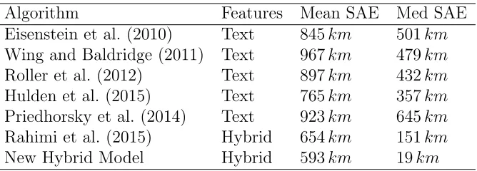
We achieve a median prediction error of only 19 km on the test data set, considerably better than most of the literature. Although the hybrid model is multi-modal by default, our algorithm maintains highly accurate single point estimates. In addition, we have a mean SAE of 593 km, which also outperforms the other algorithms in Table 2.1. The difference in the mean and median SAEs indicates that the origin of some tweets are highly difficult to predict, skewing the overall results.

(36)

Table 2.1: The simple accuracy error metric compared to the literature using the Eisen-stein data set from 2010. Results are reported in kilometers using the great-circle distance function.

Algorithm Features Mean SAE Med SAE

Eisenstein et al. (2010) Text 845km 501km Wing and Baldridge (2011) Text 967km 479km Roller et al. (2012) Text 897km 432km Hulden et al. (2015) Text 765km 357km Priedhorsky et al. (2014) Text 923km 645km Rahimi et al. (2015) Hybrid 654km 151km

New Hybrid Model Hybrid 593km 19km

in the literature by a factor of nearly 8. Recall, the method presented by Rahimi et al. [2015] uses the text and network features sequentially. The authors use the text features to predict locations without a network and then perform spatial label propagation to finish the algorithm. Our model, on the other hand, uses both features jointly and weights each according to their geographic distribution. Spatial label propagation is competitive with our hybrid algorithm [Compton et al., 2014]. However, the authors heavily filter the data and only predict approximately 10% of the data for competitive results. Our algorithm is able to successfully predict nearly 99% of the test data.

To account for the geographic distribution of subpopulation mixtures, the comprehen-sive accuracy error (CAE) is a measure of the expected distance between the true origin of the tweet and a random point generated from the model. There is no requirement for subpopulations to be clustered near each other for hpy|m, njq to be a good estimator.

(37)

CAE “Ehrdpy, y1qs “

ż

y

dpy, y1qhpy|m, njqdy . (2.6)

To estimate the integral in Equation (2.6) we use the Monte Carlo method, CAE «

1

|z|

ř

yPzdpy, y

1_q_{, where}_z _{is a sample from}_h_p_y_|_{m, n}

jqof size 100 in our testing.

Theprediction region area, denotedP RAα, is the area encompassed by 100ˆ p1´αq%

density of hpy|m, njq. There are multiple ways to calculate P RAα. We sum the area

covered by the highest 100ˆ p1´αq% density of each mixture contributing tohpy|m, njq.

The area of each mixture is calculated as a function of α and its covariance matrix Σ,

πχ2₂pαqdetpΣq1{2 .

A small prediction region is ideal yet unserviceable if it rarely covers the true location. Therefore the P RAα performance is assessed concurrently with the coverage, COVα, or

the proportion of times the prediction region covers the true origin of the tweet. To calculate COVα, we simply measure the proportion of times the true origin of the tweet

is within the ellipses defined by P RAα for the test set. A geographic point y1 “ py11, y21q is within the boundary of an ellipse with center µand covariance matrix Σ if

py1´µqTΣ´1py1´µq ďχ22pαq.

The comprehensive accuracy error, prediction region area, and coverage metrics are unique to models with geographic distribution estimates. As a result, Table 2.2 compares these metrics with Priedhorsky et al. [2014] only.

(38)

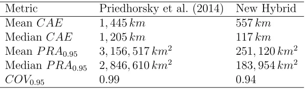
Table 2.2: The comprehensive accuracy error, prediction region area, and coverage met-rics compared to Priedhorsky et al. [2014] because both algorithms use Guassian mixture models. The weighting scheme applied by Priedhorsky et al. [2014] is the sum of the product of the elements in each covariance matrix of each GMM.

Metric Priedhorsky et al. (2014) New Hybrid

Mean CAE 1,445km 557km

Median CAE 1,205km 117km

Mean P RA0.95 3,156,517km2 251,120km2 Median P RA0.95 2,846,610km2 183,954km2

COV0.95 0.99 0.94

point generated from our model is less than 117 km, 50% of the time. Similar to the discrepancy between the mean and median SAE, the difference between the mean and median CAE indicate the predictions are skewed. However, this simply means that some subpopulations in hp¨q are a large distance from one another. For example, if a person moves from Atlanta, Georgia to Las Vegas, Nevada, it is likely the hybrid model will estimate a subpopulation for each location, causing the CAE to be large by default. More importantly, the bimodal structure of the model captures both possible locations.

The mean and median P RA0.95 are approximately 200,000km2. Although this is a large geographic area, it is more than ten times smaller than theP RA0.95 of Priedhorsky et al. [2014]. To make it tangible, consider that the median prediction region of Pried-horsky et al. [2014] is more than a third of the contiguous United States. The median prediction region for the hybrid model, on the other hand, is approximately the geo-graphic area of only North and South Carolina combined. Additionally, the coverage for the hybrid model is nearer to the nominal level in our experiments, whereas the previ-ous method has much higher than nominal coverage due to extremely large prediction regions.

(39)

and methodology underestimated this metric by 3 – 14%. We eventually chose to sum the area covered by the highest 100ˆ p1´αq% density of each mixture contributing to

the hybrid model. This technique achieves a coverage nearly equal to the nominal rate and also keeps the prediction region area metric small.

Coverage is also closely associated with the outlier preprocessing described in Sec-tion 2.4. Failure to remove outliers widens the Gaussian mixture model’s predicSec-tion re-gions causing the coverage to inflate. We also examined the effectiveness of removing observations

farther than 200 miles from at least 5 other observations,

within a cluster of less than five observations where the number of subpopulations

is determined by the “elbow” phenomenon in the K-means clustering algorithm.

We ultimately chose to remove observations from both text and network variables farther than the mean distance from their respective subpopulation center. Although this tech-nique provides similar results to the aforementioned methods, it is an automated routine for removing outliers.

2.7 Application

(40)

(ILI) reports. That is, the frequency of influenza keywords are used as a proxy for the true rate of influenza among US citizens.

In Brazil, researchers are using Twitter to monitor the rate and study the diffusion of Dengue fever, a mosquito-borne illness that can lead to death if untreated. In countries without efficient government agencies to monitor the spread of disease, it is important for researchers to develop tools that can identify regions of disease outbreak in order to allocate resources properly. Gomide et al. [2011] use geotagged tweets relevant to Dengue fever to cluster data into regions. The frequency of tweets is used as a barometer for the severity of Dengue fever within each region. In an effort to utilize more informa-tion, Davis Jr et al. [2011] classify non-geotagged tweets at the city level using network information. This allows the authors to use Dengue fever relevant tweets that are not geotagged in their analyses.

In both applications, influenza in the United States and Dengue fever in Brazil, the hybrid method is advantageous. First, the hybrid method allows practitioners to geotag more data because both the text and network features are available to be used as possible predictors. In our experiments in Section 2.6, the hybrid method was able to geotag 98.2% of test tweets. Using text or network features independently, only 79.7% and 90.1% of test tweets were able to be geotagged respectively. Furthermore, the use of model uncertainty provides more information regarding the location of disease outbreak. That is, the smaller the prediction regions of the hybrid method, the more confident we are in the estimated location. Additionally, the greater the certainty in the location of a set of geotagged tweets, the greater the evidence for allocating resources to specific regions.

(41)

the 376,510 tweets, only 1,031 contain influenza related keywords. As evidenced by the performance metrics, the hybrid model can be used to accurately predict the location of influenza related tweets. However, the uncertainty associated with the estimates is ignored if the best predictions are simply binned into regions.

To account for the uncertainty in the predictions, suppose that we stack the geographic density estimates,hp¨q, for each predicted tweet and reweight to obtain a final geographic probability distribution of the prevalence of influenza throughout the country. Let hqp¨q

be the qth hybrid model density estimate of a sample of non-geotagged tweets S. The final distribution which combines all predictions and uses the uncertainty of each is ř|S|

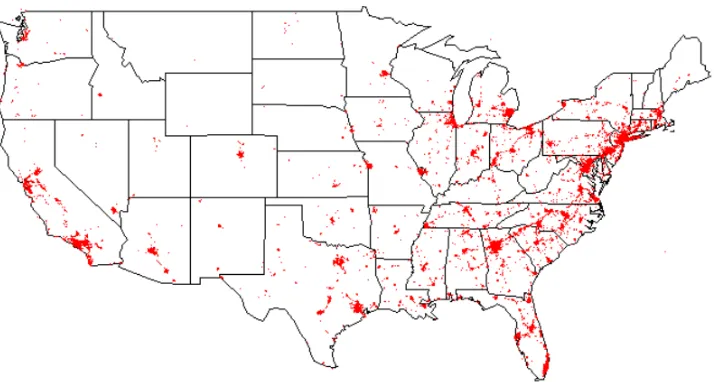
q“1hqp¨q{|S|. Figure 2.5 displays the estimated distribution of influenza in the United States during March of 2010 according to the Eisenstein data set.

Figure 2.5: Geographic probability distribution of influenza in the United States during March of 2010.

(42)

the week the Eisenstein data was collected. In general, these reports summarize by re-gion the percent of medical patients with influenza like illness, percent testing positive for influenza, and the number of jurisdictions reporting influenza activity. For the first week of March, only region 1 (CT, ME, MA, NH, RI, VT) and region 4 (AL, FL, GA, KY, MS, NC, SC, TN) reported widespread influenza activity. In addition, the Midwest and Southwest experienced sporadic influenza activity, and the Northwest reported no influenza activity. The report is similar to the estimated distribution in Figure 2.5. That is, there is elevated influenza in the northeast and southeast regions. In addition, there is activity in the Midwest and no activity in the Northwest. However, Figure 2.5 indi-cates possible elevated influenza activity in southern California; the CDC report does not support this finding.

Note, the results here do not simply imitate the most dense locations of Twitter users from the Eisenstein data set (Figure 2.4). Also, Twitter usage has grown significantly since the data was collected in 2010, but there is no reason to suspect the application is no longer suitable.

2.8 Conclusion

In this chapter we presented a hybrid geolocation model for Twitter. Our model exploits both text and network features and weights the features according to their geographic scope. Our method outperforms other geotagging algorithms according to four metrics. In particular, the median distance between the most probable location to the origin of a single tweet is only 19 km on average in our experiments.

(43)

within a spatial domain of being the origin of a tweet. This structure allows us to visually interpret model confidence for a single tweet (Figure 2.3) or combine the uncertainty for a set of geotagged tweets to monitor an event such as influenza (Figure 2.5).

Any analysis of Twitter data is subject to the biases and limitations of the data itself. The limitations of Twitter data in general are attributable to the demographics of its users, Twitter’s streaming API sampling scheme, and users turning off their location services when tweeting. First, a 2012 investigation by the Pew Research Center found that age is inversely related to the likelihood of using Twitter [Duggan and Brenner, 2013]. Internet users in the age group 18-29 are the most likely to use Twitter, and users 65 or older are the least likely. Women are more likely than men and urban residents are more likely than suburban or rural dwellers to use Twitter. Also, different levels of education and levels of household income correspond to similar rates of Twitter use. As a result of the Pew study, we know any data gathered from Twitter does not mimic the population in general.

To obtain a free sample from Twitter any person can connect to the streaming API and download approximately 1% of all tweets daily. Procuring additional tweets is a substantial cost and therefore, most researchers opt for the free sample. However, the algorithm used to sample from the streaming API is currently unknown and may not be uniformly random. Morstatter et al. [2013] show that tweets collected freely are gen-erally biased according to trending topics and the most used hashtag strings. One final additional point of concern is that to our knowledge there is no study describing the user demographics for those who are more willing to leave the Twitter location services turned on. There may be revealing information simply from tweets with or without geotags.

(44)

(45)

Chapter 3 Dynamic Logistic Regression

Variable Selection

3.1 Overview

(46)

model features. We show improved accuracy of forecasting protests compared to the cur-rent baseline approach and report the most common predictive terms to contextualize the reasons for civil unrest. The accuracy of the variable selection technique used for the application is demonstrated by means of simulation.

3.2 Introduction

Dynamic linear models (DLMs) are utilized for forecasting complex non-stationary time series. Originally developed within engineering in the 1960s [Petris et al., 2009], a variety of applications can now be found in, for example, ecology [Calder et al., 2003], medicine [West et al., 1999], and finance [Koop and Korobilis, 2012]. The time-varying parameters of these state space regression models allow for greater flexibility in short-term forecast-ing. The time-varying structure allows for parameters to evolve along with structural changes in a system over time. In addition, the intrinsic Bayesian framework of DLMs allows for sequential and efficient updating of model parameters as new information be-comes available.

Consider the univariate DLM specified by the observation equation (Equation 3.1a) and state equation (Equation 3.1b) for tě1,

Yt “Xtβt`vt vt„Np0, σ2q, (3.1a)

βt “Gtβt´1`wt wt„Np0,Wq. (3.1b)

Yt is the observed scalar at time t, βt is the p-dimensional parameter vector (also called

(47)

matrix governing the system disturbances, or the changes in the true underlying model. In addition, vt and wt are two independent sequences of independent Gaussian errors

with mean zero and known variance components.

Fitting dynamic linear models has become somewhat straightforward with modern computing power and MCMC techniques, so more recent work focuses on effect selection, or determining which elements of βt are nonzero at each successive time point t. With

applications in finance, such as equity premium and inflation forecasting [Kalli and Grif-fin, 2014], it is common to have a high-dimensional state vector where many elements are unrelated to the target. Erroneous effects may reduce prediction accuracy and hin-der model inference. This has spurred efforts to intelligently remove irrelevant predictors from hypothesized models. Because DLMs have advantageous properties in the Bayesian framework, such as sequentially updating the model as new information becomes avail-able, many of the variable selection methods rely on sparsity-promoting priors. These are priors that shrink parameters towards zero if evidence suggests the predictors are unassociated with the target [Park and Casella, 2008]. Variable selection techniques will be discussed more fully in Sections 3.3 and 3.4.

(48)

environmen-tal statistics to monitor pollutant exposure [Chiogna et al., 2002], medicine to monitor surgical outcomes [McCormick et al., 2012], and engineering to monitor the output of a machine [Raftery et al., 2010].

Although a powerful and flexible modeling tool for non-Gaussian time series data, DGLMs have received far less attention in the literature than their predecessor, the DLM. One possible reason is that exponential family distributions are more challenging to model in the dynamic scenario. Moving away from Gaussian distributions causes on-line estimation of states, or sequential updating of model parameters, to become more difficult. In fact, most of the research pertaining to DGLMs focuses on simply fitting the model. Techniques include MCMC based approaches [Gamerman, 1998], data augmen-tation [Windle et al., 2013], and online estimation of states [West et al., 1985], which inevitably requires some degree of approximation to maintain real-time estimation.

As a result of the challenges posed from simply fitting the DGLM, little attention has been given to DGLM variable selection. One of the only DGLM variable selection methods uses a variation of Bayesian model averaging techniques [Raftery et al., 2010], which does not scale efficiently as the number of predictors grows. There is simply not a rich set of variable selection methods for the DGLM as there are with static linear models, static generalized linear models, or even dynamic linear models. In this chapter, we present a variable selection method for the dynamic logistic regression model. The

observation equation for this DGLM can be specified as

yt|βt„Bernoullipπtq, πt“

eXtβt

1`eXtβt t “1, . . . , T , (3.2)

where the response yt P t1,0u represents a “success” or “failure” respectively at time t,

(49)

equation is the same as in the DLM scenario in Equation 3.1b.

Although the motivation for this problem exists in both literature and application, as described above, our specific interest comes from the article “Combining Heterogeneous Data Sources for Civil Unrest Forecasting” [Korkmaz et al., 2015]. In this work, the au-thors seek to forecast the probability of protest events in six South American countries using open sources of information as model features including social media, blogs, news, and currency exchange rates. The authors use logistic regression coupled with LASSO regularization to forecast the probability of civil unrest and find Twitter key words are commonly selected as model predictors. We seek to improve upon the forecast perfor-mance by accounting for dependencies in successive observations and the possibility of changing model features over time. We also seek to find a sparse representation of the model as the application is within thepąn scenario and to better infer the reasons for civil unrest.

(50)

3.3 Static Variable Selection Methods

We briefly describe some of the more popular techniques for variable selection in both the Bayesian and non-Bayesian literature. Some of the more recent methods for static models (both linear and generalized linear) are the basis for variable selection in the dynamic linear model.

First, consider the traditional linear model,

Y “Xβ`, (3.3)

where Y is the n-dimensional observation vector, X is the n ˆp design matrix, β “

pβ1, . . . , βpq is the p-dimensional vector of model parameters, and error „ Np0,Σ “

σ2_I

nq.

For linear regression, information criteria such as AIC [Akaike, 1974] and BIC [Schwarz, 1978] are used to compare a set of hypothesized models. These metrics assess model fit according to the maximum value of the likelihood function and are penalized by the number of estimated predictors,

AIC “2k´2 log`Lˆpβq˘ and BIC “logpnqk´2 log`Lˆpβq˘.

Here, k is the number of estimated parameters, n is the number of observations, and ˆ

Lp¨q is the evaluated likelihood. The penalties discourage overfitting because goodness of fit inevitably improves as the number of predictors increases. The AIC and BIC are measures of the tradeoff between goodness of fit and model dimension. The preferred model from the candidate set is the one with the lowest information criteria.

(51)

forward and backward selection. In forward selection, one begins with the null model and iteratively adds parameters until the information criteria is no longer reduced. Backward selection is the opposite. It begins with all parameters in the model and iteratively removes parameters until the information criteria is no longer reduced.

Forward and backward selection can be combined into stepwise selection, where pa-rameters can be added or removed at each step. The advantage of stepwise selection is that it is an automated process of choosing model predictors. However, stepwise selection does not always improve prediction accuracy. To overcome this pitfall, Tibshirani [1996] introduced the least absolute shrinkage and selection operator (LASSO). This technique involves altering the model fitting process itself by penalizing the likelihood function. β

is chosen to minimize

Lpβq “kY ´Xβk2

2`λPpβq,

where λ is a threshold chosen by cross-validation and Ppβq “kβk1 is the regularization penalty. The constraint imposed on the likelihood function is used to avoid over fitting the model. The constraint forces some parameters to zero, effectively resulting in a more interpretable model. Due to the success of the LASSO method, a variety of other penalized likelihood functions have been proposed by alteringPpβq, including group LASSO [Yuan

and Lin, 2006], adaptive LASSO [Zou, 2006], fused LASSO [Tibshirani et al., 2005], elastic net [Zou and Hastie, 2005], smoothly clipped absolutely shrinkage and selection operator [Fan and Li, 2001], and the Dantzig selector [Candes and Tao, 2007]. Each penalty provides its own unique advantage regarding regularization.

(52)

ap-proaches are all readily exploitable in existing software. For example, the R package

glmnet fits generalized linear models with the LASSO penalty, kβk1, the ridge penalty, kβk2

2, and a linear combination of the two known as elastic net, p1´λqkβk1`λkβk22. In parallel to non-Bayesian approaches, Bayesian variable selection for both linear regression and generalized linear models has proceeded similarly. Motivated by classical hypothesis testing, Bayes factors are used as a model comparison and selection tool. For example, consider comparing the plausibility of two models, M1 and M2. Kass and Raftery [1995] suggest computing the posterior odds of the two models,

πpM1|Yq πpM2|Yq “

πpY|M1q πpY|M2q

πpM1q πpM2q ,

where the equation above can be interpreted as posterior odds = Bayes factors ˆ

prior odds. A large value of the posterior odds suggests support for the model M1 compared to model M2.

Considering a set ofK models,pM1, . . . , MKq, it is commonplace to choose and deploy

the model with the best posterior odds after a series of pairwise comparisons. However, choosing a single best model may be inadequate. Suppose the other K ´1 models also

provide a reasonably good fit to the data as well. Hoeting et al. [1999] suggest Bayesian model averaging (BMA) to incorporate information from each plausible model. That is, simply weight the prediction from each model, ˆYMk, by the posterior model probability,

ErYˆ|ys “

K

ÿ

k“1 ˆ

YMkπpMk|Yq.

Averaging predictions in BMA allows practitioners to better account for model uncer-tainty [Hoeting et al., 1999].

(53)

probabilities for each is infeasible. Methods such as Gibbs variable selection (GVS) [Dellaportas et al., 2002] and stochastic search variable selection (SSVS) [George and McCulloch, 1993] have been proposed to avoid enumerating all possible models. These approaches introduce latent variables,I “ pI1, . . . , Ipq, into the model whereIj “1

indi-cates predictor j is included in the model. Conditional on the latent variables, mixture prior distributions are placed on the model parameters,πpβ|Iq. More commonly, the prior is referred to as “spike-and-slab”. The “spike” refers to the probability Ij ‰ 0 and the

“slab” refers to the prior distribution attributed to βj. Using MCMC techniques, these

methods sample through the model space identifying posterior inclusion probabilities of each parameter, which can then be used for variable selection.

More recent literature has focused on adaptive shrinkage priors to achieve effect selec-tion. These prior distributions shrink elements ofβ towards zero if the data support the claim βj “0 and avoid shrinkage for data supported evidence of βj ‰0. The priors are

adaptive in the sense that regularization adheres to data-driven evidence and the degree of regularization can be tuned by altering prior distribution parameters, a concept similar to altering the threshold parameterλ in non-Bayesian regularization. For example, Park and Casella [2008] propose the Laplace prior which assumes a hierarchical prior for βj,

βj|τj „Np0, τjq τj „exppδq.

In this case, the degree of sparseness, or simply the number of βj “ 0, is tuned by the

hyper-parameter δ. This method is referred to as the Bayesian LASSO.

To obtain even greater control over the degree of sparseness, Griffin et al. [2010] suggest using the Normal-Gamma prior. Again, conditional onτj,βj „Np0, τjqand now

(54)

gives greater control over the shrinkage of model parameters. Specifically, asλ decreases, more prior mass is placed close to zero while simultaneously maintaining heavy tails in the distribution. This allows for greater shrinkage and also, allows estimated coefficients to vary in magnitude with less restriction.

3.4 DLM and DGLM Variable Selection Methods

Recall that the univariate DLM is specified by the observation equation and state equa-tion as given in Equaequa-tions 3.1a and 3.1b.

From a non-Bayesian perspective, the only dynamic model variable selection methods reside in the compressed sensing (CS) literature. In general, CS refers to reconstructing a signal in underdetermined linear systems, or simply thepąn paradigm. Static CS mod-els use variable selection techniques such as LASSO. Angelosante et al. [2009] consider dynamic compressed sensing, with time varying parameters, and propose the dynamic LASSO,

argmin β1,...,βt

T

ÿ

t“1

kyt´Xtβtk22 subject to

T

ÿ

t“1

kβtk1 ďλ ,

where λ is the tuning parameter controlling the degree of sparseness.

Apart from compressed sensing, the rest of the dynamic model selection literature is strictly Bayesian. The Bayesian framework allows for efficient sequential updating of the state vector as new information becomes available. In fact, compressed sensing practition-ers have even started to apply Bayesian methodology citing the ease of implementation [Sejdinovic et al., 2010].

(55)

dynamic model averaging (DMA) and Koop and Korobilis [2012] apply the methodology to forecast inflation. The key difference between BMA and DMA is that DMA allows the true model to vary in time. The model observation equation and state equation are specified as

yt“X

pkq

t β

pkq

t `v

pkq

t v

pkq

t „Np0, σ2pkqq,

β_tpkq“G_tpkqβ_tp_´kq₁`w_tpkq w_tpkq „Np0,Wpkq q,

wherekdenotes the model index. DMA requires calculating the probability of each model being the true model at timetand averaging forecasts using posterior model probabilities,

Eryˆt|y1:t´1s “

K

ÿ

k“1 ˆ

ytpkqπpMk|y1:t´1q.

As before, considering all possible 2p _{models is not feasible, and as a result, both}

BMA and DMA consider only a small set of candidate models. More recent and efficient Bayesian approaches rely on fitting the model with all parameters and shrinking ele-ments of βt toward zero in accordance with the data. Motivated by the “spike-and-slab”

approach, Nakajima and West [2013] propose shrinking parameters to zero if their abso-lute value falls below a threshold at any point in time t. This latent threshold modeling (LTM) approach introduces a matrix of latent variables, It “diagpI1t, . . . , Iptq, into the

observation equation,

yt“XtpItβtq `vt vt „Np0, σ2q,

where Ijt “Ip|βjt| ě djq and dj ě0 for all p. The degree of sparseness is controlled by

(56)

A few adaptive shrinkage priors have been discussed in the DLM literature. Motivated by the shrinkage methodology of Park and Casella [2008], Belmonte et al. [2014] extend the Bayesian LASSO to the DLM. The authors first break the observation equation into both static parameters, β, and dynamic parameters, βt,

yt “Xtβ`Xtβt`vt vt „Np0, σ2q.

Then, Bayesian LASSO shrinkage is applied to both the static coefficients, β, and the variance components of the state equation, W “diagpσ2₁, . . . , σ2_pq. That is,

βj|τj „Np0, τjq τj „exppδjq,

σ_j2|ξj „Np0, ξjq ξj „exppγjq.

Due to the altered state equation and the shrinkage priors, there are three possible post model fitting scenarios.

Ifσ_j2 and βj are shrunk to zero, then predictorj is removed from the model.

Ifσ2

j is shrunk to zero but βj is not shrunk to zero, then parameter βj is static.

Ifσ_j2 is not shrunk to zero, then parameter βj is considered dynamic.

Thus, the authors not only seek a parsimonious model but also an understanding of which parameters are static versus dynamic.

(57)

βt|τ „Npµ, τΣq τ „GiGausspν, δ, γq,

where µP Rp,Σ is a pˆpcovariance matrix, and GiGaussp¨qis the generalized inverse

Gaussian distribution [Barndorff-Nielsen and Shephard, 2001]. Lettingβj “ pβj1. . . , βjTq

denote the evolution of the jth _{parameter, then} _β

j P RT follows the multivariate

gener-alized hyperbolic distribution, which simplifies to static model adaptive shrinkage priors under specific parameterizations. For example, if δ “ 0 and ν “ 1 the prior reduces to the Laplace prior of Park and Casella [2008]. Likewise, if δ “ 0, ν ‰ 1, and ν ą 0 the prior reduces to the Normal-Gamma prior of Griffin et al. [2010].

The final adaptive shrinkage prior in the DLM literature is referred to as the Normal-Gamma Autoregressive (NGAR) process [Kalli and Griffin, 2014]. As its name implies, this prior is motivated by the Normal-Gamma prior of Griffin et al. [2010] with an extension to the DLM. Again, for this process denoteβj “ pβj1. . . , βjTqas the evolution

of the jth predictor coefficient. The process is written βj „ N GARpλj, µj, ϕj, ρjq, with

the NGAR process for βj defined as

κjpt´1q|ψjpt´1q „ P oisson

ˆ

ρjpλj{µjqψjpt´1q

1´ρj

˙ ,

ψjt|κjpt´1q „ Gamma

ˆ

λj `κjpt´1q,

λj

µjp1´ρjq

˙ ,

ηjt|ψjt „ N

`

0,p1´ϕ2_jqψjt

˘ ,

βjt “

d ψjt

ψjpt´1q

ϕjβjpt´1q`ηjt, t“1, . . . , T .

The process begins withψj0 „Gammapλj, λj{µjqand βj0|ψj0 „Np0, ψj0q.

(58)

parameter λj controls the degree of sparseness. Small values of λj place more prior mass

at zero and cause heavier shrinkage for thejth_{coefficient. The autocorrelation parameters}

ρj and ϕj control the dependence between ψjpt´1q and ψjt, as well as βjpt´1q and βjt

respectively. Thus,ρj and ϕj control the ability for the importance of parameters to vary

in time.

There is only one dynamic generalized linear model variable selection method present in the literature. McCormick et al. [2012] extend the dynamic model averaging approach of Raftery et al. [2010] to the dynamic logistic regression model. Given a set ofK candi-date models, pM1, . . . , MKq, and letting Lt be the model indicator at time t, the

obser-vation equation becomes

yt|Lt“Mk„Bernoullipp

pkq

t q, and logitpp

pkq

t q “X

pkq

t β

pkq

t .

The forecasts from each of the K models are then averaged using πpLt “ Mk|y1:t´1q as weights.

3.5 Model Fitting

(59)

3.5.1 Fitting the Dynamic Linear Model

Recall, the univariate DLM is specified by the observation equation and state equation

Yt “Xtβt`vt vt„Np0, σ2q,

βt “Gtβt´1`wt wt„Np0,Wq,

where Yt is the observed scalar at time t, βt is the p-dimensional state vector, Xt is a

vector of known covariates, and the errors vt and wt are two independent sequences of

independent Gaussian errors with mean zero and known variance components. We will assume Gt is the identity matrix, which implies each element of the state vector varies

according to a random walk.

From this representation, it is easy to see that the DLM satisfies the following as-sumptions.

βt is a Markov chain.

Conditionally on βt, the observable Yt’s are independent.

As a result, the DLM is completely specified by the initial distribution πpβ0q and the conditional densities πpβt|βt´1q and πpyt|βtq,

πpβ0:T,y1:Tq “πpβ0q

T

ź

i“1

πpβi|βi´1qπpyi|βiq. (3.7)

Assuming the initial distribution πpβ0q and the conditional densities πpβt|βt´1q and πpyt|βtqare all Gaussian, then it can be shown the random vectorpβ0,β1, . . . ,βt, Y1, . . . , Ytq

(60)

by their means and variances. As a result, the filtering distributions can be computed sequentially as new information becomes available using the Kalman filter. The solution of filtering the DLM, or updating the state vector Gaussian distribution, is as follows [Petris et al., 2009]. Begin by lettingβt´1|y1:t´1 „Npmt´1,Ct´1q.

The one step ahead predictive distribution ofβt|y1:t´1 is Gaussian with parameters

at“Epβt|y1:t´1q “Gtmt´1 , Rt “V arpβt|y1:t´1q “GtCt´1G1t`W . (3.8)

The one step ahead predictive distribution ofYt|y1:t´1 is Gaussian with parameters

ft “EpYt|y1:t´1q “ Xtat, Qt“V arpYt|y1:t´1q “XtRtXt1`σ

2 _. _(3.9)

The filtering distribution of βt|y1:t is Gaussian with parameters

mt“Epβt|y1:tq “ at`RtXt1Q

´1

t et , Ct“V arpβt|y1:tq “ Rt´RtXt1Q

´1

t XtRt,

(3.10)

where et“Yt´ft is the forecast error.

The Kalman filter detailed above assumes the variance components of the observation equation and state equation are known. Assuming σ2 _and _W _{are unknown, the joint} distribution is specified as

πpβ0:t, σ2,W,y1:tq “πpβ0q ˆπpWq ˆπpσ2q ˆ

t

ź

i“1

πpβi|βi´1,Wq ˆπpyi|βi, σ2q. (3.11)

Twitter Analytics: Geotag Imputation, Forecasting, and Dynamic Variable Selection.

ABSTRACT

DEDICATION

BIOGRAPHY

ACKNOWLEDGEMENTS

CONTENTS

LIST OF TABLES

LIST OF FIGURES

Chapter 1

Introduction and Motivation

1.1

Geotag Imputation

1.2

Forecasting and Dynamic Variable Selection

1.3

Measurement Error

Chapter 2

Geotag Imputation: A Hybrid

Approach

2.1

Overview

2.2

Introduction

2.3

Related Work

2.3.1

Text Approaches

2.3.2

Network Approaches

2.3.3

Hybrid Approach

2.4

Preprocessing

2.4.1

Text Preprocessing

2.4.2

Text and Network Preprocessing

2.5

New Hybrid Model

2.6

Results

2.6.1

Data

2.6.2

Performance Metrics

2.7

Application

2.8

Conclusion

Chapter 3

Dynamic Logistic Regression

Variable Selection

3.1

Overview

3.2

Introduction

3.3

Static Variable Selection Methods

3.4

DLM and DGLM Variable Selection Methods

3.5

Model Fitting

3.5.1

Fitting the Dynamic Linear Model