Application of structural equation models to construct genetic networks using differentially expressed genes and single nucleotide polymorphisms

Open Access

Proceedings

Application of structural equation models to construct genetic

networks using differentially expressed genes and single-nucleotide

polymorphisms

Seungmook Lee

_{, Mina Jhun}

_{, Eun-Kyung Lee}

_{and Taesung Park*}

Address: 1_{Department of Statistics, Seoul National University, San 56-1, Sillim-dong, Gwanak-gu, Seoul 151-742, Korea and} 2_{Interdisciplinary}

Program in Bioinformatics, Seoul National University, San 56-1, Sillim-dong, Gwanak-gu, Seoul 151-742, Korea Email: Seungmook Lee - [email protected]; Mina Jhun - [email protected]; Eun-Kyung Lee - [email protected]; Taesung Park* - [email protected]

* Corresponding author

Abstract

Understanding the genetic basis of human variation is an important goal of biomedical research. In this study, we used structural equation models (SEMs) to construct genetic networks to model how specific single-nucleotide polymorphisms (SNPs) from two genes known to cause acute myeloid leukemia (AML) by somatic mutation, runt-related transcription factor 1 (RUNX1) and ets variant gene 6 (ETV6), affect expression levels of other genes and how RUNX1 and ETV6 are related to each other. The SEM approach allows us to compare several candidate models from which an explanatory genetic network can be constructed.

Background

To understand the genetic basis of complex traits, it is often useful to examine intermediate gene expression traits. It is known that many diseases occur because of changes in either patterns or levels of gene expression [1,2]. There are also known cases in which differences in gene expression due to genotype are associated with phenotypic variation [3-7]. Thus, the analysis of gene expression may lead to a better understanding of the genetic basis of complex traits [3]. The study of gene expression variation, both within and

between species, is currently an active area of research [8-10].

We propose an approach based on structural equation models (SEMs) [11] to construct a genetic network that can provide information about the genetic basis of expression variation in humans. SEMs were originally developed in the early 1970s in the field of social science to fit models with unobserved variables. A key feature of the SEM approach is that it allows one to compare candidate mod-els.

from Genetic Analysis Workshop 15

St. Pete Beach, Florida, USA. 11–15 November 2006

Published: 18 December 2007

BMC Proceedings 2007, 1(Suppl 1):S76

<supplement> <title> <p>Genetic Analysis Workshop 15: Gene Expression Analysis and Approaches to Detecting Multiple Functional Loci</p> </title> <editor>Heather J Cordell, Mariza de Andrade, Marie-Claude Babron, Christopher W Bartlett, Joseph Beyene, Heike Bickeböller, Robert Culverhouse, Adrienne Cupples, E Warwick Daw, Josée Dupuis, Catherine T Falk, Saurabh Ghosh, Katrina A Goddard, Ellen L Goode, Elizabeth R Hauser, Lisa J Martin, Maria Martinez, Kari E North, Nancy L Saccone, Silke Schmidt, William Tapper, Duncan Thomas, David Tritchler, Veronica J Vieland, Ellen M Wijsman, Marsha A Wilcox, John S Witte, Qiong Yang, Andreas Ziegler, Laura Almasy and Jean W MacCluer</editor> <note>Proceedings</note> <url>http://www.biomedcentral.com/content/pdf/1753-6561-1-S1-info.pdf</url> </supplement>

This article is available from: http://www.biomedcentral.com/1753-6561/1/S1/S76

© 2007 Lee et al; licensee BioMed Central Ltd.

In this study, we used gene expression data and SNP data provided by the Genetic Analysis Workshop 15 (GAW15). The study subjects were selected from 14, three-generation Utah families with ancestry from northern and western Europe (Utah Centre d'Etude du Polymorphisme Humain, or CEPH). Each family consisted of 14 individuals (4 grandparents, 2 parents, and 8 offspring), except for two families that had only 7 offspring (so only 13 individuals). In these families, expression levels of 8500 genes in lym-phoblastoid cells were initially measured. Morley et al. [12] found that 3554 genes out of these 8500 genes showed greater variations among individuals than between repli-cate determinations in the same individual. Expression lev-els of these 3554 genes were provided to GAW15. The GAW15 genotype data contained 2882 autosomal and X-linked single-nucleotide polymorphisms (SNPs) for each member of the 14 CEPH Utah families. The genotypes were generated by the SNP Consortium http://snp.cshl.org/.

We are interested in acute myeloid leukemia (AML). In this study, we focused on two known AML-related genes,

runt-related transcription factor 1 (RUNX1) and ets variant gene

6 (ETV6). Although expression levels for these two genes

were not included in the GAW15 data set, we used two-way analysis of variance (ANOVA) models to find other genes that were differentially expressed depending on the

geno-type for SNPs within RUNX1 and ETV6. Using genes

selected from the ANOVA, we fitted SEMs and constructed genetic networks.

Methods

Selection of differentially expressed genes from SNPs

First, we used dbSNP (Build 126) and the Online Mende-lian Inheritance in Man (OMIM) FTP site of the National Center for Biotechnology Information (NCBI) to select

SNPs within RUNX1 and ETV6. Next, we used the

follow-ing model to fit two-way ANOVA models to find differen-tially expressed genes for each selected SNP:

y_ijk = μ+ FAMID_i + SNP_j + FAMID*SNP_ij + ε_ijk,

where y_ijk is the expression level of the gene in the kth

indi-vidual with SNP genotype j from family i. FAMID and SNP

represent the family and SNP effects, respectively, and εijk is

a random error term. A gene was selected to be part of the SEM analysis if the fit of the full model was significantly

better (p < 0.05) than the model that included only overall

mean and family.

Structural equation models for genetic networks

SEMs are comprehensive statistical models that allow us to test relations among observed and latent variables; in this context, we used them to construct a network of differen-tially expressed genes for specific polymorphisms. Latent variables are unobserved variables that are implied by the

covariance among two or more indicators. The expression

levels for RUNX1 and ETV6 were not included in the data

provided to GAW15. Because of this, and the way we selected our observed variables, we believe it is likely that the latent variables represent the level of expression of these two genes.

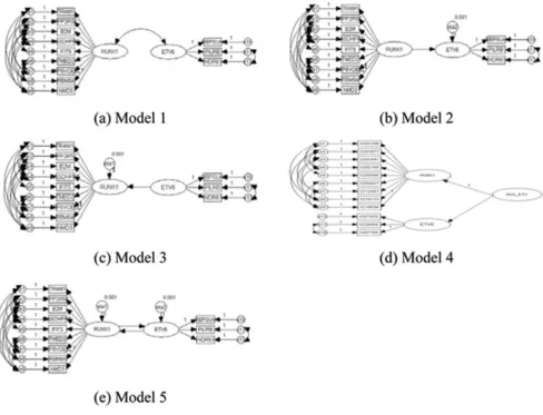
Path diagrams were used to describe genetic networks in a graphical manner (Figure 1). There are two types of varia-bles used in path diagrams: observed variavaria-bles (represented by rectangles) and latent variables (represented by ovals). The relationships defined in SEMs consist of two parts: rela-tionships among the latent variables and relarela-tionships between the latent variables and the observed variables. The SEMs for our genetic networks were defined as follows:

y = Λ_yη+ ε,

η= Bη+ ς,

where y is a vector representing the observed variables

(gene expression levels); ηis a vector of the latent variables

(RUNX1 and ETV6 expression); Λy is a matrix representing

the true relationships between the gene expression levels

and the gene functions; and B is a matrix representing the

true the relationships among the latent variables. Random

errors in the equations are represented by εand ς. To fit this

model, we used AMOS, a SEM software solution provided by SPSS http://www.spss.com/amos/.

Results

From the 2882 SNPs provided in the GAW15 data set, we

identified six SNPs located on RUNX1 and ETV6 on the

basis of chromosomal location. The RUNX1 SNPs are

rs882776, rs933131, and rs1892687 and the ETV6 SNPs

are rs1894307, rs1573612, and rs916041.

Although we selected SNPs based solely on physical

posi-tion, we expect that RUNX1 and ETV6 are co-regulated and

are involved in the regulation of additional genes. We con-structed the SEMs after identifying genes apparently regu-lated by these six SNPs.

Construction of a genetic network for differentially expressed genes using SEMs

From our ANOVA analyses, we identified nine differen-tially expressed genes associated with the RUNX1 SNPs:

translocation associated membrane protein 1 (TRAM1);

gamma isoform (PPP2R5C); beta-2-microglobulin (B2M);

aminoadipate-semialdehyde

dehydrogenase-phospho-pantetheinyl transferase (AASDHPPT); interferon-induced

protein with tetratricopeptide repeats 5 (IFIT5);

transmem-brane emp24 domain trafficking protein 2 (TMED2);

(ATP6V0E2L); RNA binding motif protein 8A (RBM8A); and NMD3 homolog (NMD3). Similarly, we identified

three genes with expression correlated to the ETV6 SNPs:

recombining binding protein suppressor of hairless (

RBP-SUH); paired immunoglobin-like type 2 receptor beta

(PILRB); and WD repeat domain 61 (WDR61). Figure 2 shows the box plots of expression levels for these 12 selected genes.

First, we applied confirmatory factor analysis [11] to vali-date the use of these 12 differentially expressed genes in our SEM. Then, we added the relation between the latent variables and fitted the general SEMs.

To construct the genetic network, we treated RUNX1 and

ETV6 as latent variables and all genes with expression val-ues as observed variables. We considered SEMs where both

RUNX1 and ETV6 could control any of the 12 expressed genes.

We fitted various SEMs to the data, as shown in Figure 1. Model 1 assumes that there is a correlation between the two latent variables and Models 2 and 3 assume that there is a one-sided causal relationship between them. Model 4 is a second-order factor model in which the latent variables directly influencing the observed variables may be influ-enced by other latent variables that need not have direct effects on the observed variables [11]. Finally, Model 5 assumes that there are mutual causal relationships between the two latent variables.

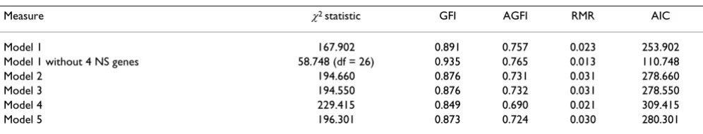
Table 1 shows goodness-of-fit measures for the five models. The goodness-of-fit index (GFI) measures the relative dif-ferences between data and estimated values obtained from a model, while the adjusted GFI (AGFI) adjusts the GFI according to the degrees of freedom. If these two measures are close to 1, we conclude that the model fits the data well. Smaller root mean square residuals (RMRs) indicate better-fitting models. The Akaike information criterion (AIC) is a Diagram of SEMs for constructing genetic structures

Figure 1

well-known measure that can be used for the model com-parison. A smaller AIC indicates a better-fitting model.

For Models 1–5, we tested, using the modification index (MI), many modified SEMs with different covariance structures for the error terms. The MI measures how much the chi-square statistic is expected to decrease if a particu-lar constrained parameter is set free and the model is re-estimated [11]. In our model fitting, we first evaluated all pair-wise error connections and chose the connection with the largest MI. Given the first connection, we then chose the best remaining possible connection, and so forth. We continued until the improvement in fit was small.

Figure 1 illustrates the models that best fit the covariance structure for the error terms. Table 1 summarizes goodness of fit measures for these models. Model 1 provided the best fit, yielding the largest GFI and AGFI and the smallest AIC. For Models 2, 3, and 5, the estimates of the error variances were negative, indicating that these models represent the so-called "Heywood cases" [11]. Model 4 provided the best result in terms of the RMR but the worst result in terms of other goodness-of-fit measures such as the AIC. Because the AIC and RMR are different measures of goodness-of-fit, they might provide inconsistent results. One advantage of the AIC is that it considers the number of parameters in the

model, while the RMR does not. Thus, we selected Model 1 as the best model in terms of the AIC.

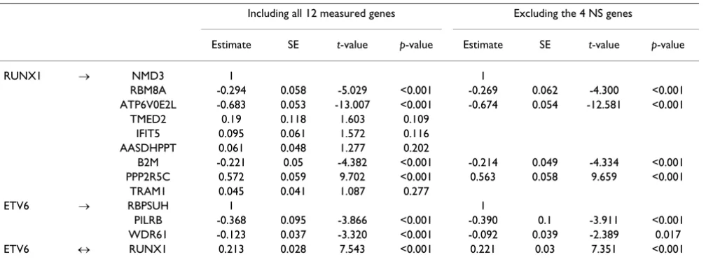
The fitted results of Model 1 are summarized in Table 2; the results show that the latent variables we believe represent

RUNX1 and ETV6 expression are closely related to each other. The parameter relating these latent variables (Table

2) estimates the covariance between RUNX1 and ETV6.

Of the 12 genes with measured expression, all three that

were differentially expressed for ETV6 showed significant

connection to the latent variable representing ETV6.

Among the nine differentially expressed genes for RUNX1,

four – TMED2, IFIT5, AASDHPPT, and TRAM1 – did not

show significant control by the latent variable RUNX1.

When we excluded these nonsignificant genes, the good-ness-of-fit measures improved compared to the full Model 1 (Table 1) while the parameter estimates and significance (Table 2) remained similar to those of the full model.

Conclusion

In this paper, we proposed the use of SEMs to construct genetic network models. We demonstrated this method

using two genes, RUNX1 and ETV6, which are well known

to cause AML by somatic mutation [13]. We used SNPs in these genes to select the differentially expressed genes related to these SNPs to use as the observed variables for our SEMs. The best-fitting model indicated that, even

Table 1: Goodness-of-fit measures for SEMs

Measure χ2 _{statistic GFI AGFI RMR AIC}

Model 1 167.902 0.891 0.757 0.023 253.902 Model 1 without 4 NS genes 58.748 (df = 26) 0.935 0.765 0.013 110.748 Model 2 194.660 0.876 0.731 0.031 278.660 Model 3 194.550 0.876 0.732 0.031 278.550 Model 4 229.415 0.849 0.690 0.021 309.415 Model 5 196.301 0.873 0.724 0.030 280.301 Box plot of selected gene expressions

Figure 2

though we did not have direct measurements of RUNX1

and ETV6 expression, they are likely to be highly correlated with each other.

In summary, SEMs allow us to compare candidate models and to construct a genetic network from the best fitting model. However, the SEM approach has several limitations, such as 1) as the number of genes increases, the number of parameters in the model can increase exponentially; 2) if there are many genes, it is difficult to determine the causal-ity relationship among the genes; 3) it can be difficult to interpret the relationship embedded in SEMs. For these rea-sons, in order to construct the genetic network efficiently, it is very useful to find a few genes that are correlated with other genes in the proposed network. Another limitation of the SEM approach is that it requires the selection of an ini-tial model that is updated to construct the final SEM. As described above, this process can require many iterations to determine an appropriate error structure. In spite of these limitations, we believe that our application of SEMs to the GAW15 data demonstrates that the SEM approach can be a useful and efficient method for constructing informative genetic networks.

Competing interests

The author(s) declare that they have no competing inter-ests.

Acknowledgements

This work was supported by the National Research Laboratory Program of Korea Science and Engineering Foundation (M10500000126). The authors thank the editor and two anonymous referees, whose comments were extremely helpful.

This article has been published as part of BMC Proceedings Volume 1 Supple-ment 1, 2007: Genetic Analysis Workshop 15: Gene Expression Analysis and Approaches to Detecting Multiple Functional Loci. The full contents of the

supplement are available online at http://www.biomedcentral.com/1753-6561/1?issue=S1.

References

1. Wilson AC, Maxson LR, Sarich VM: Two types of molecular evolu-tion: evidence from studies of interspecific hybridization. Proc Natl Acad Sci USA 1974, 71:2843-2847.

2. Wray GA, Hahn MW, Abouheif E, Balhoff JP, Pizer M, Rockman MV, Romano LA: The evolution of transcriptional regulation in eukaryotes. Mol Biol Evol 2003, 20:1377-1419.

3. Schadt EE, Monks SA, Drake TA, Lusis AJ, Che N, Colinayo V, Ruff TG, Milligan SB, Lamb JR, Cavet G, Linsley PS, Mao M, Stoughton RB, Friend SH: Genetics of gene expression surveyed in maize, mouse and man. Nature 2003, 422:297-302.

4. Oleksiak MF, Churchill GA, Crawford DL: Variation in gene expres-sion within and among natural populations. Nat Genet 2002, 32:261-266.

5. Townsend JP, Cavalieri D, Hartl DL: Population genetic variation in genome-wide gene expression. Mol Biol Evol 2003, 20:955-963. 6. Brem RB, Yvert G, Clinton R, Kruglyak L: Genetic dissection of transcriptional regulation in budding yeast. Science 2002, 296:752-755.

7. Toma DP, White KP, Hirsch J, Greenspan RJ: Identification of genes involved in Drosophila melanogaster geotaxis, a complex behavioral trait. Nat Genet 2002, 31:349-353.

8. Johnson NA, Porter AH: Allelic variation in human gene expres-sion. J Theor Biol 2000, 205:527.

9. Levine M: Evolutionary biology:how insects lose their limbs.

Nature 2002, 415:848.

10. Xiong M, Li J, Fang X: Identification of genetic networks. Genet

2004, 166:1037-1062.

11. Bollen KA: Structural Equations with Latent VariablesNew York: John Wiley & Sons, Inc; 1989.

12. Morley M, Molony CM, Weber T, Devlin JL, Ewens KG, Spielman RS, Cheung VG: Genetic analysis of genome-wide variation in human gene expression. Nature 2004, 430:743-747.

13. Horwitz AF, Hunter T: Cell adhesion: integrating circuitry. Trends Cell Biol 1996, 6:460-461.

Table 2: Parameter estimates for Model 1

Including all 12 measured genes Excluding the 4 NS genes

Estimate SE t-value p-value Estimate SE t-value p-value

RUNX1 → NMD3 1 1

RBM8A -0.294 0.058 -5.029 <0.001 -0.269 0.062 -4.300 <0.001 ATP6V0E2L -0.683 0.053 -13.007 <0.001 -0.674 0.054 -12.581 <0.001

TMED2 0.19 0.118 1.603 0.109 IFIT5 0.095 0.061 1.572 0.116 AASDHPPT 0.061 0.048 1.277 0.202

B2M -0.221 0.05 -4.382 <0.001 -0.214 0.049 -4.334 <0.001 PPP2R5C 0.572 0.059 9.702 <0.001 0.563 0.058 9.659 <0.001

TRAM1 0.045 0.041 1.087 0.277

ETV6 → RBPSUH 1 1