R E S E A R C H
Open Access
The joint effects of diffusion and delay on
the stability of a ratio-dependent
predator-prey model
Kejun Zhuang
1,2*and Gao Jia
3*Correspondence:
1Business School, University of
Shanghai for Science and Technology, Shanghai, 200093, China
2School of Statistics and Applied
Mathematics, Anhui University of Finance and Economics, Bengbu, 233030, China
Full list of author information is available at the end of the article
Abstract
This paper is concerned with a diffusive and delayed predator-prey system with Leslie-Gower and ratio-dependent Holling type III schemes subject to homogeneous Neumann boundary conditions. Preliminary analyses on the well-posedness of solutions and the dissipativeness of the system are presented with assistance of inequality technique. Then the Hopf bifurcation induced by spatial diffusion and time delay is discussed, respectively. Moreover, the bifurcation properties are obtained by computing the norm forms on the center manifold. Finally, some numerical
simulations and conclusions are given to verify and illustrate the theoretical results.
MSC: 35K57; 35B32; 92D25
Keywords: predator-prey system; Hopf bifurcation; reaction-diffusion system; delay
1 Introduction
In population ecology, the dynamics of species populations and the way these populations interact with the environment have raised widespread concerns []. It is the study of how the population sizes of species change over time and space. Among these interactions, the predator-prey interaction is the most basic one, and plenty of mathematical models have been established since the pioneering work by Lotka and Volterra [, ].
To better understand the relationship between predator and prey, a functional re-sponse is utilized to model the intake rate of a consumer as a function of food density, such as Holling types I-IV [, ], Beddington-DeAngelis type [], Hassell-Varley type [], Leslie-Gower type [], Crowley-Martin type [], and so on [, ]. In many situations, when predators have to search, share or compete for their resources, the so-called ratio-dependent functional response is reasonable. It means that the per capita predator growth rate is a function of the ratio of prey to predator abundance. This is strongly supported by numerous fields and laboratory experiments and observations []. Such ratio-dependent models can present rich dynamic behaviors, see [–]. In addition, the environmental carrying capacity of predator is proportional to the number of prey; consequently, the Leslie-Gower type functional response was proposed in [, ].
For most populations, they do not always stay in a fixed place and usually move from a higher concentration region to a lower concentration one. Thus, the spatial diffusive factor
should be considered in modeling the predator-prey system. Given all this, a nondimen-sional diffusive Leslie-Gower predator-prey model with ratio-dependent Holling type III functional response was considered in [] as follows:
⎧ ⎨ ⎩
∂u(x,t)
∂t –du(x,t) =u(x,t)( –u(x,t)) –
βu(x,t)v(x,t)
u(x,t)+mv(x,t), x∈,t> ,
∂v(x,t)
∂t –dv(x,t) =rv(x,t)( – v(x,t)
u(x,t)), x∈,t> .
Here,u(x,t) andv(x,t) represent the density of the prey and predator at timetand loca-tionx∈, respectively. The region⊂RN (N≤) is a bounded domain with smooth
boundary ∂. The nonnegative continuous initial conditions and homogeneous Neu-mann boundary conditions are imposed. All the coefficients are positive constants,dand
dare diffusion coefficients, and more detailed ecological meanings can be found in [].
As is well known, time delay, especially the maturation delay of the predator, is ubiq-uitous in an ecological system. Hence, in this paper, by taking account of the combined effects of spatial diffusion and time delay, we mainly consider the following modified predator-prey model:
⎧ ⎪ ⎪ ⎪ ⎪ ⎪ ⎨ ⎪ ⎪ ⎪ ⎪ ⎪ ⎩
∂u(x,t)
∂t –du(x,t) =u(x,t)( –u(x,t)) –
βu(x,t)v(x,t)
u(x,t)+mv(x,t), x∈,t> ,
∂v(x,t)
∂t –dv(x,t) =rv(x,t)( – v(x–τ,t)
u(x–τ,t)), x∈,t> , ∂u(x,t)
∂ν = ∂v(x,t)
∂ν = , x∈∂,t> ,
u(x,t) =u(x,t)≥, v(x,t) =v(x,t)≥, x∈,t∈[–τ, ],
()
where all the coefficients are positive constants, time delayτ> is the mature time of the predator. The initial functionsu(x,t) andv(x,t) are continuous,∂/∂νrepresents the
out-ward normal derivative on the boundary∂. The system is subject to no-flux boundary conditions, and it means that the ecology system is self-contained. In fact, there have been some significant results about the simplifications of system (). In detail, the spatiotempo-ral dynamics have been studied without time delay. For example, Shi and Li [] focused on the local and global stability of positive constant steady state by using the linearization method and the Lyapunov functional method. In [], Shi et al. derived the existences of Turing bifurcation, Hopf bifurcation, and Turing-Hopf bifurcation by regardingras the bifurcation parameter. In [], Zhou also investigated the existence of Turing pattern and nonexistence of nonconstant steady state solutions by the bifurcation method and the en-ergy method. Besides, Song et al. [] considered the corresponding delay system without diffusion and ratio-dependent functional response and established the existence of local and global Hopf bifurcations by choosing time delay as the bifurcation parameter. For some other related results, refer to [–].
for determining the Hopf bifurcation properties. In Section , we conduct some numeri-cal simulations to illustrate our theoretinumeri-cal results. Finally, we give some conclusions and biological interpretations.
2 Elementary results
Here, we establish some basic properties of the solutions of system (), specifically, the well-posedness of solutions and the dissipativeness of system ().
For convenience, we first restate a useful lemma from [] as follows.
Lemma Consider the equation
⎧ ⎪ ⎪ ⎨ ⎪ ⎪ ⎩
∂w
∂t =Dw+wg(w(x,t–τ)), x∈,t> , ∂w
∂ν = , x∈∂,t> ,
w(x,s)≥, w(x, )≡, x∈,s∈[–τ, ].
()
If the function g satisfies g(w)≤α( –w/d),then the solution of()has the property
lim sup t→+∞
max
w(·,t)≤deατ.
Theorem System()has a unique global solution,and the solution remains nonnegative and uniformly bounded for all t> .
Proof Following the process in [, ], we can similarly get the local existence and uniqueness of solution (u(x,t),v(x,t)) withx∈andt∈[,T), whereT is the maximal existence time of the solution.
In order to conform to the comparison theorem and the standard theory of semilinear parabolic system in [], we only need to construct a pair of coupled lower-upper solutions
= (, ) and M = (M,M) , where
M=max
, sup –τ≤s≤
u(·,s)C(,¯R)
,
M=max
Merτ, sup –τ≤s≤
v(·,s)C(,¯R).
Then the proof can be completed.
In the following, we will show that any nonnegative solution of system () is bounded as t→+∞for allx∈.
Theorem (Dissipativeness) The system()is dissipative.That is,the nonnegative solu-tion(u,v)of system()satisfies
lim sup t→+∞
u(x,t)≤, lim sup t→+∞
v(x,t)≤erτ.
Proof On the basis of positivity of solutions in Theorem , we have
∂u(x,t)
∂t –du(x,t)≤u(x,t) –u(x,t)
Then we can estimate the upper limit ofu(x,t) due to the standard comparison principle:
lim sup t→+∞
u(x,t)≤.
In other words, for an arbitraryε> , there exists a positive constantTsuch that for any
t≥T,
u(x,t)≤ +ε.
Analogously, for anyT∈[T+τ, +∞), we have
∂v(x,t)
∂t –dv(x,t)≤rv(x,t)
–v(x,t–τ) +ε
.
Therefore, the following estimation can be deduced by Lemma :
lim sup
t→+∞ v(x,t)≤e
rτ.
The proof is complete.
3 The stability of positive steady states and the existence of Hopf bifurcation Setting the right sides of the first two equations in system () equal to zero and solving the algebraic equations ofuandv, we can obtain the two constant steady states:E= (, )
andE∗= (u∗,v∗), whereu∗=v∗= – +mβ . Apparently,E∗is positive when the following
assumption holds:
(H) β< +m.
So, we always expect assumption (H) to be true. For the convenience of research, in the remainder of this paper, we only consider the one-dimensional region= (,lπ).
We know that the eigenvalues of the operator –onunder the homogeneous Neu-mann boundary conditions areμn=n/l,n= , , , . . . . LetE(μn) be the eigenfunction
space corresponding toμninC(),{ϕnj:j= , , . . . ,dimE(μn)}be an orthonormal basis
ofE(μn),X= [C()], andXnj={c·ϕnj: c∈R}. Then
X=
∞
n=
Xn and Xn= dimE(μn)
j=
Xnj.
For eachn≥,Xnis invariant under the linearized operator of system (), and the
char-acteristic equation atE= (, ) is given by
λ+dn
l +
(+m)–β
(+m)
β(–m) (+m)
–r λ+dn
l +r
= ,
which is equivalent to
λ+d
n
l +
λ–d
n
l –r
The constant steady state is asymptotically stable if all the characteristic values have nega-tive real parts for anyn≥. It is evident that characteristic equation () has a positive value λ=rwhenn= . Then the semi-trivial steady stateE= (, ) is always unstable. From the
ecological point of view, we are more interested in the stability of positive constant steady stateE∗= (u∗,v∗), and the corresponding characteristic equation is
In the following, we shall explore the effect of spatial diffusion and time delay on the dynamic behaviors of system (), respectively.
3.1 The effect of diffusion
In this subsection, we regard coefficientβ as the bifurcation parameter and discuss the effect of spatial diffusion on the stability of positive steady state E∗ without time delay.
Then the characteristic equation () can be reduced to
λ–Tnλ+Dn= , ()
Through direct computation, we can obtain the following inequality when the positive constant steady state exists:
For anyn≥ withτ = , the necessary condition for the existence of Hopf bifurcation at E∗isTn= , that is,
β– ( +m)( +r)
( +m) = (d+d)
n
l.
Denote
βn=
( +m)(d +d)n
l + ( +m)( +r)
, n= , , , . . . ,
then the positive steady stateE∗is asymptotically stable whenβ<βand the potential
Hopf bifurcation may occur whenβ>β.
Next, we need to verify the transversality condition. Suppose that the root of equation () has the formλ(β) =a(β) +ib(β). Substituting it into () and separating the real and negative parts, we get
a(β)b(β)i=Tnb(β)i,
and
Re λ(β)=a(β) =T
n(β)
=
( +m) > .
We further make the following assumption:
(H) ( +m)( +r) < .
With the previous analysis, the following conclusions can be drawn by the Hopf bifurca-tion theory in [].
Theorem When hypotheses(H)and(H)are satisfied,we have
(i) Ifβ∈(,β),then the positive steady stateE∗is asymptotically stable.
(ii) Ifβ∈(β,m+ ),then the positive steady stateE∗is unstable.
(iii) The periodic solutions bifurcating fromβ=βare spatially homogeneous,and the
periodic solutions bifurcating fromβ=βn(≤n≤N,βN<m+ ,βN+≥m+ )
are spatially inhomogeneous.
3.2 The effect of delay
Next, we discuss the dynamic behaviors ofE∗by taking time delayτ as the bifurcation parameter.
Let±iω(ω> ) be the roots of equation (), then we get
–ω+iωAn+Bn+ (cosωτ–isinωτ)(iωC+Fn) = .
Separating the real and imaginary parts can lead to
⎧ ⎨ ⎩
ω–Bn=Fncosωτ+ωCsinωτ,
–ωAn=ωCcosωτ–Fnsinωτ,
and
() has the unique positive rootωn, and the characteristic equation () has purely
imagi-nary roots±iωn, where
By solving equations (), we get
⎧
and then obtain the corresponding values ofτ as follows:
τ=τj(n)=
To verify the transversality condition, we take the derivative of equation () with respect toτ and have
It can be simplified to
and
Re
dλ dτ
–
τ=τj(n)
= ω
n+Fn–Bn
(Fnωn)+ (Cωn)
.
Denote
(H) β<min{m+ , ( +m)/}.
If condition (H) holds, thenFn+Bn=Dn> . Moreover, from
Fn–Bn= –dd
n
l +
rd–d+
dβ
( +m)
n
l +
r( +m–β)
+m ,
we can always find the greatest nonnegative integerN, such that
Fn–Bn> , forn= , , , . . . ,N.
Therefore, we get
Re
dλ dτ
–
τ=τj(n)
> .
From above, we can establish the existence of Hopf bifurcation induced by time delay.
Theorem When hypothesis(H)is satisfied,we have
(i) Forτ ∈[,τ),the positive steady state(u∗,v∗)is asymptotically stable. (ii) orτ>τ,the positive steady state(u∗,v∗)is unstable.Furthermore,τ=τj(n)
(j= , , , . . .;n= , , , . . . ,min{N,N})are Hopf bifurcation values.
4 Bifurcation properties
In this section, we mainly analyze the direction of the Hopf bifurcation and the stability of the bifurcating periodic solutions obtained in Theorem . The methods here are based on the center manifold theorem and normal form theory for partial functional differential equations in [, ].
In general, we use τ∗ to denote an arbitrary value of τj(n) with j ∈ N and n ∈ {, , , . . . ,min{N,N}}. And we also use±iω∗to denote the corresponding simply purely
imaginary roots±iωn.
Settingu(˜ ·,t) =u(·,τt),v(˜·,t) =v(·,τt),U(t) = (˜ u(˜ ·,t),˜v(·,t)), andτ=τ∗+αwithα∈R, thenα= is the Hopf bifurcation value of system (). For simplicity, we drop the tilde and rewrite system () in the form
dU(t)
dt =τDU(t) +L(α)(Ut) +f(Ut,α), ()
whereD=diag{d,d},ϕ= (ϕ,ϕ)T∈C, andL(α)(·) :C→X,f :C×R→Xare given by
L(α)(ϕ) = τ∗+α
β–(+m)
(+m) ϕ() –β(–m)(+m)ϕ()
rϕ(–) –rϕ(–)
f(ϕ,α) = τ∗+α
From Section , we can know that±iω∗τ∗is a pair of simple purely imaginary eigenval-ues of the following linear differential equation:
˙
U(t) =τDU(t) +L(α)(Ut). ()
Next, we discuss the following differential equation:
˙
Y(t) = –τDnY(t) +L(α)(Yt). ()
By the Riesz representation theorem here, there exists a × matrix functionη(θ,α) (–≤θ≤) whose elements are of bounded variation such that
–τDn
ThenA∗ andAare adjoint operators under the bilinear form
It can be verified that q(θ) = q()· eiω∗τ∗θ = (,η)Teiω∗τ∗θ (θ ∈ [–, ]) and q∗(s) =
valuedLinner product on the Hilbert spaceX Cis
Settingα= , we can obtain the center manifold
W(z,z,¯ θ) =W
The flow of system () on the center manifold can be written as follows:
Ut= q(θ)z(t) +q(θ)¯z(t)
Following the calculation procedures in [] and [], we can get
and
E=E×
F+F|η|+F(η+η)
E
cosnx
l ,
E=|η|(G+G) +G+ GRe
ηeiω∗τ∗
+ |η|GRe
eiω∗τ∗+ G
Re{η},
E=
dn
l –
β–(+m)
(+m)
β(–m) (+m)
–r dn
l +r
–
.
From the above analysis, we can compute the following quantities which determine the direction of bifurcation and the stability of periodic solutions:
c() =
i ω∗τ∗
gg– |g|–
|g|
+g ,
= –
Re(c()) Re(λ(τ∗)),
ι= Re c()
,
χ= –
ω∗τ∗ Im c()
+Im λ τ∗
.
Theorem For system(),
(i) determines the bifurcation direction:if> ,then the bifurcation is supercritical
and the periodic solution exists forτ>τ;if< ,then the bifurcation is subcritical
and the periodic solution exists forτ<τ.
(ii) ιdetermines the stability of bifurcating periodic solutions:the periodic solutions are
orbitally asymptotically stable ifι< ,or unstable ifι> .
(iii) χdetermines the period of the bifurcating periodic solutions:the period is
monotonically increasing at time delayτ whenχ> ,or is monotonically
decreasing at time delayτ whenχ< .
5 Numerical simulations
In this section, to illustrate the analytic results, we will conduct some numerical examples by the aid of MATLAB.
For system (), we set
= (,π), m= ., r= ., d= , d= .,
and choose the initial functionsu= . + .sin(x+t) andv= + .sin(x+t), then we
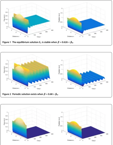
can get the unique Hopf bifurcation valueβ= .. Thus, the bifurcating periodic
so-lutions are spatially homogeneous. From Theorem , we can find that the positive equilib-rium solutionE∗≈(., .) is asymptotically stable whenβ= . <β(see
Fig-ure ), and the periodic solution bifurcates fromE∗≈(., .) whenβ= . >β
(see Figure ). From Figure , the solutions converge to zero, and a periodic phenomenon vanishes whenβis slightly away from the critical valueβbecause the Hopf bifurcation
Figure 1 The equilibrium solutionE∗is stable whenβ= 0.626 <β0.
Figure 2 Periodic solution exists whenβ= 0.68 >β0.
Figure 3 Solution converges to zero whenβ= 0.8 >β0.
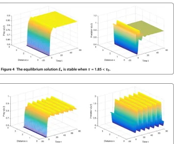
Next, to meet the assumption (H), we rechoose
m= , β= ., r= ., d= , d= .,
and the initial functionsu= . andv= . Then the positive equilibrium solution is
E∗= (., .). By direct computation, we have the Hopf bifurcation critical value τ≈. whenn= andω≈.. From Figures and , we can observe that
the positive equilibrium solutionE∗is asymptotically stable when time delayτ = . is smaller than the Hopf bifurcation critical valueτ; on the other hand,E∗is unstable, and
Figure 4 The equilibrium solutionE∗is stable whenτ= 1.85 <τ0.
Figure 5 The equilibrium solutionE∗is unstable, and a periodic solution occurs whenτ= 3 >τ0.
Figure 6 The spatially inhomogeneous periodic solution exists.
Finally, from Figure , we can also observe the existence of spatially inhomogeneous periodic solution when
m= , β= ., r= ., d= ., d= ., τ=
with initial valuesu= . + .cos(x+t) andu= + .cos(x+t).
6 Conclusions
been established based on inequality techniques. Hopf bifurcation conditions have also been derived by choosing different bifurcation parameters respectively. It is observed that a periodic phenomenon appears when the bifurcation parameter passes through some critical value.
It is shown that the parameterβ, which reflects the specific predation rate or the in-teraction strength between two species, can make the equilibrium solutionE∗= (u∗,v∗)
asymptotically stable or unstable without time delay. From Theorem , we can control the parameterβ sufficiently small to achieve the stabilization. For example, some mea-sures can be adopted to decrease the value ofβ, such as founding a refuge for prey species or increasing the interference with interaction between two species. On the other hand, the numerical examples indicate that a spatially homogeneous periodic solution will exist when the parameterβis larger than the Hopf bifurcation value. Nevertheless, whenβis far away from the critical value, the two species will be extinct. It reflects that over-hunting or denudation may seriously destroy the ecological environment.
Our results also show that time delay has a vital impact on the dynamics of system (). The second group of parameters we choose in Section also satisfy the conditions of Theorem . in []. That is to say, the equilibrium solutionE∗is globally asymptotically
stable when time delay is equal to zero. However, the asymptotic behavior is not able to always keep stable when time delay varies. If time delayτ is sufficiently small, then the equilibrium solutionE∗is still asymptotically stable. Whenτ is slightly larger than a cer-tain critical value, the equilibrium solutionE∗is no longer stable and a spatially periodic
solution may appear. Furthermore, if we choose other diffusion coefficients, we can find spatially inhomogeneous periodic solutions, which are not included in [, ], without time delay.
Well, due to the local existence of Hopf bifurcation, the periodic solutions only exist in a small neighborhood of bifurcation value. It is interesting and significant to further explore the global continuation of local Hopf bifurcation, which can ensure the existence of periodic solutions when the parameter is much larger or less than the bifurcation value. We will continue this research in the near future. Still, the methods and results in the present paper have supplemented the ones in [–] and can also be applied to other reaction-diffusion systems without or with time delay. We hope that our work could be useful to study the effects of spatial diffusion and time delay on the population dynamics.
Competing interests
The authors declare that they have no competing interests.
Authors’ contributions
Both authors contributed equally in this article. They read and approved the final manuscript.
Author details
1Business School, University of Shanghai for Science and Technology, Shanghai, 200093, China.2School of Statistics and
Applied Mathematics, Anhui University of Finance and Economics, Bengbu, 233030, China.3College of Science,
University of Shanghai for Science and Technology, Shanghai, 200093, China.
Acknowledgements
This work is supported by the National Natural Science Foundation of China (11301001 and 11171220). It is also supported by the Key Project for Excellent Young Talents Fund Program of Higher Education Institutions of Anhui Province (gxyqZD2016100) and the Anhui Provincial Natural Science Foundation (1508085MA09 and 1508085QA13).
Received: 10 November 2016 Accepted: 19 January 2017
References
2. Lotka, AJ: Elements of Physical Biology. Williams & Wilkins, Baltimore (1925)
3. Goel, NS, Maitra, SC, Montroll, EW: On the Volterra and other nonlinear models of interacting populations. Rev. Mod. Phys.43, 232-276 (1971)
4. Dawes, J, Souza, MO: A derivation of Holling’s type I, II and III functional responses in predator-prey systems. J. Theor. Biol.327, 11-22 (2013)
5. Li, Y, Xiao, D: Bifurcations of a predator-prey system of Holling and Leslie types. Chaos Solitons Fractals34, 606-620 (2007)
6. Haque, M: A detailed study of the Beddington-DeAngelis predator-prey model. Math. Biosci.234, 1-6 (2011) 7. Hsu, SB, Hwang, TW, Kuang, Y: Global dynamics of a predator-prey model with Hassell-Varley type functional
response. Discrete Contin. Dyn. Syst., Ser. B10, 857-871 (2008)
8. Mohammadi, H, Mahzoon, M: Effect of weak prey in Leslie-Gower predator-prey model. Appl. Math. Comput.224, 196-204 (2013)
9. Tripathi, JP, Tyagi, S, Abbas, S: Global analysis of a delayed density dependent predator-prey model with Crowley-Martin functional response. Commun. Nonlinear Sci. Numer. Simul.30, 45-69 (2016)
10. Wang, X, Wei, J: Diffusion-driven stability and bifurcation in a predator-prey system with Ivlev-type functional response. Appl. Anal.92, 752-775 (2013)
11. Hu, D, Cao, H: Stability and bifurcation analysis in a predator-prey system with Michaelis-Menten type predator harvesting. Nonlinear Anal., Real World Appl.33, 58-82 (2017)
12. Arditi, R, Ginzburg, LR: Coupling in predator-prey dynamics: ratio-dependence. J. Theor. Biol.139, 311-326 (1989) 13. Zhang, L, Liu, J, Banerjee, M: Hopf and steady state bifurcation analysis in a ratio-dependent predator-prey model.
Commun. Nonlinear Sci. Numer. Simul.44, 52-73 (2017)
14. Banerjee, M, Abbas, S: Existence and non-existence of spatial patterns in a ratio-dependent predator-prey model. Ecol. Complex.21, 199-214 (2015)
15. Sharma, S, Samanta, GP: A ratio-dependent predator-prey model with Allee effect and disease in prey. J. Appl. Math. Comput.47, 345-364 (2015)
16. Leslie, PH: Some further notes on the use of matrices in population mathematics. Biomtrika35, 213-245 (1948) 17. Leslie, PH: A stochastic model for studying the properties of certain biological systems by numerical methods.
Biomtrika45, 16-31 (1958)
18. Shi, H, Li, Y: Global asymptotic stability of a diffusive predator-prey model with ratio-dependent functional response. Appl. Math. Comput.250, 71-77 (2015)
19. Shi, H, Ruan, S, Su, Y, Zhang, J: Spatiotemporal dynamics of a diffusive Leslie-Gower predator-prey model. Int. J. Bifurc. Chaos25, 1530014 (2015)
20. Zhou, J: Bifurcation analysis of a diffusive predator-prey model with ratio-dependent Holling type III functional response. Nonlinear Dyn.81, 1535-1552 (2015)
21. Song, Y, Yuan, S, Zhang, J: Bifurcation analysis in the delayed Leslie-Gower predator-prey system. Appl. Math. Model.
33, 4049-4061 (2009)
22. Banerjee, M, Zhang, L: Influence of discrete delay on pattern formation in a ratio-dependent prey-predator model. Chaos Solitons Fractals67, 73-81 (2014)
23. Fang, L, Wang, J: The global stability and pattern formations of a predator-prey system with consuming resource. Appl. Math. Lett.58, 49-55 (2016)
24. Camara, BI, Haque, M, Mokrani, H: Patterns formations in a diffusive ratio-dependent predator-prey model of interacting populations. Physica A461, 374-383 (2016)
25. Yang, R, Zhang, C: Dynamics in a diffusive predator-prey system with a constant prey refuge and delay. Nonlinear Anal., Real World Appl.31, 1-22 (2016)
26. Tian, Y: Stability for a diffusive delayed predator-prey model with modified Leslie-Gower and Holling-type II schemes. Appl. Math.59, 217-240 (2014)
27. Hattaf, K, Yousfi, N: A generalized HBV model with diffusion and two delays. Comput. Math. Appl.69, 31-40 (2015) 28. Hattaf, K, Yousfi, N: Global dynamics of a delay reaction-diffusion model for viral infection with specific functional
response. Comput. Appl. Math.34, 807-818 (2015)
29. Wu, J: Theory and Applications of Partial Functional Differential Equations. Springer, New York (1996) 30. Hassard, BD, Kazarinoff, ND, Wan, YH: Theory and Applications of Hopf Bifurcation. Cambridge University Press,