Block sparsity based localization in wireless sensor networks

R E S E A R C H

Open Access

Block-sparsity-based localization in wireless

sensor networks

Alessandro Bay

, Diego Carrera

, Sophie M. Fosson

, Pasqualina Fragneto

, Marco Grella

, Chiara Ravazzi

and Enrico Magli

Abstract

In this paper, we deal with the localization problem in wireless sensor networks, where a target sensor location must be estimated starting from few measurements of the power present in a radio signal received from sensors with known locations. Inspired by the recent advances in sparse approximation, the localization problem is recast as a block-sparse signal recovery problem in the discrete spatial domain. In this paper, we develop different

RSS-fingerprinting localization algorithms and propose a dictionary optimization based on the notion of the coherence to improve the reconstruction efficiency. The proposed protocols are then compared with traditional fingerprinting methods both via simulation and on-field experiments. The results prove that our methods outperform the existing ones in terms of the achieved localization accuracy.

Keywords: Block-sparsity; Localization; Real data experimentation/testbed; RSS-fingerprinting

1 Introduction

In the last decade, localization services have become widespread in everyday life, supported by the advances in communication technologies that allow to detect the position of people and devices [1]. After the diffu-sion of satellite-based localization systems, which can be exploited in favorable outdoor conditions, much atten-tion has been devoted to localizaatten-tion in indoor environ-ments or in outdoor adverse conditions due to geological or energy barriers (e.g., presence of mountains or dense forests, high consumption of GPS systems) [2, 3]. The studies in this field are motivated by a number of safety and monitoring tasks, such as the tracking of products and equipment in hospitals or warehouses, or the detec-tion of security personnel in a building. More generally, tasks like indoor guidance are convenient in all those con-texts where mobility is fundamental, for example, in huge shopping malls, museums, or airports.

Localization has recently taken advantage of the devel-opment of wireless sensor networks (WSNs), that are now widely used as a valuable alternative to satellite-based technologies in the aforementioned frameworks. Many

*Correspondence: [email protected]

1Department of Electronics and Telecommunications (DET), Politecnico di Torino, Corso Duca degli Abruzzi, 24, 10129 Torino, Italy

Full list of author information is available at the end of the article

different settings, designs, and methodologies have been tested and analyzed for localization in WSNs, which are illustrated in a number of books and surveys on the topic, e.g., [3–7].

The mathematical modeling of indoor signal propaga-tion is particularly challenging due to the presence of multipath, moving elements, and reflecting surfaces. A unified approach is not available yet: techniques are typi-cally developed for a specific setting and different schemes can be combined to improve the efficiency [3].

Based on the type of measurements available, we can distinguish two main approaches: (a) triangulation and (b) scene analysis (or fingerprinting) [3]. Triangulation exploits the geometric properties of triangles and includes methods like Direction of Arrival (DoA) and Time of Arrival (ToA) (see [1] for an overview), which estimate the angle from which a source is emitting the signal and the time of arrival of the signal (which is typically proportional to the distance), respectively. Nevertheless, the former approach is not capable of revealing the physical location of the emitting source, while the second dramatically suf-fers from multipath and refraction effects. The presence of obstacles causes inaccuracies also using methods based on the measurement of the received signal strength (RSS), that is, the power transmitted by the device to be local-ized. RSS-based techniques however are more efficient if

combined with fingerprinting [8], which is a map-based approach that consists in creating a signature map in order to represent the physical space capturing the variations of the dynamic nature of the indoor radio propagation. More precisely, RSS measurements are collected off-line at some known locations in the area and then stored in a signature map. The unknown location can then be obtained on-line from the current RSS measurements, which are compared with those in the signature map.

While more robust and accurate, RSS-fingerprinting methods require the exchange of a large number of data between the receiver and the transmitter to achieve the desired level of performance. This issue has been recently tackled by recasting localization into a sparse approxi-mation problem [9–11]. The rationale is the following: assuming that the physical space is discretized onto a grid ofDcells, each of them associated with a prescribed posi-tion, the device position can be represented by a vector of lengthDthat has non-zero entries only where a device occupies that position. Typically, we want to localize few devices at a time, thus this vector has few non-zero entries, i.e., it is sparse, while the number of possible positionsD is very large. Within the aforementioned applications, the localization of a specific medical equipment in a hospi-tal [3] is an example of a problem that may be sparse. A hospital typically is a wide environment and is discretized in a huge number of cells, while a specific equipment (even if several copies of it are available) is not expected to be present everywhere, i.e., does not occupy many cells. Localization can then be performed by solving an under-determined linear system under sparsity constraints. The underlying mathematical problem is analogous to the one considered by the recent theory of compressed sensing [12], which provides a number of theoretical guarantees on the recovery accuracy.

In this paper, we start from the setting presented in [9] and we present new methods, based on block-sparsity, that improve the performance of the localization sys-tem and make it suitable for practical use. Block-sparsity assumes that the non-zero entries of the sparse signal to be reconstructed are confined in some blocks, while other segments are completely empty; recent work [13, 14] pro-vides theoretical guarantees for their reconstruction in a compressed sensing framework. Leveraging these general results, we explore RSS-fingerprinting methods based on block-sparsity and we prove their efficiency.

In particular, we propose two families of algorithms. In the first class, given the dictionary of fingerprints that consists of multiple blocks, the localization is obtained by searching for the block-sparsest solution, i.e., the repre-sentation that uses the minimum number of blocks. In the second one, the blocks are rearranged by exploiting intra-block correlation in order to improve recovery per-formance. These algorithms also shed light on how to

optimize the dictionary exploiting such correlation and, thereby, improving performance. Our criteria depend on the notion of mutual coherence of a dictionary. We evalu-ate the performance of the proposed localization systems through a number of simulations and on-field trials, show-ing their higher accuracy in terms of localization distance error with respect to the state of the art. Thanks to the blocks’ arrangement, our methods are also more robust to noise, which can be caused by interferences with other signals, or by people walking in the area, or by walls and furniture. Moreover, the algorithms we use for the local-ization are based on greedy algorithms, which are known to be computationally efficient. Thus we obtain a more accurate localization in a short time, as we will explain at the end of Section 3.

The paper is organized as follows: in Section 2, we introduce the localization scenario, defining the setting of our model; in Section 3, we explain the proposed algo-rithms based on block-sparsity. Technical details on the boards used in our experiments and the validation of the theoretical model are given in Section 4. Finally, the results of simulations and field tests, both in outdoor and indoor environments, are presented in Sections 5 and 6, respectively.

2 Indoor localization system

In this section, we introduce the localization scenario that we consider throughout the paper and we describe the mathematical formulation of the problem.

2.1 Model setting

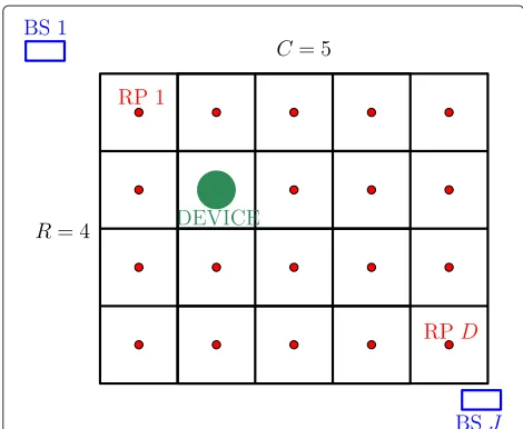
We start by defining a two-dimensional regionA ⊂ R2 that represents the area of interest where the device to be localized is placed. We then consider a discretization of Aby settingD∈Nsignificant points inA, named refer-ence points (RPs), whose coordinates are indicated byξi, i∈ {1,. . .,D}, and partitioningAintoDsubsets (or cells), each of them containing a RP. If the environment is pretty much uniform, a natural choice to arrange the cells is a uniform grid that covers the entire area with the desired resolution, as in Fig. 1. On the other hand, if obstacles such as building walls or furniture limit the area, non-uniform adapted partitions could be considered. The RPs are generally intended as the centroids of the cells. For simplicity of exposition, in this work, we always consider a rectangular-shaped regionAwith uniform grid ofRrows andCcolumns, andD=RCRPs as in Fig. 1.

Fig. 1Example of a uniform grid over a rectangular area_A; the RPs (red dots) are set in the centroids of the cells; in this case the BSs are set outside_A

and runs the localization algorithm. In our model, the BSs are assumed to acquire the RSS of the signals, which is a measure of the power. RSS methods are widely used for localization as they are among the most inexpensive and less consuming [9, 15]. Taking into account, the atten-uation due to the distance and obstacles between the transmitting device and the receiver (e.g., walls, furniture, and people), the RSS at distancedis modeled as follows [9]:

Pr(d)=Pt−PL(d0)−10nlog10(d/d0)−ησ, (1)

wherePtis the transmitting power,PL(d0)is the average path loss value at a reference distanced0, generallyd0 = 1m,nis an attenuation parameter (generally 2≤n≤4), ησis a zero-mean Gaussian noise with standard deviation σ, that we denote asησ ∼N(0,σ2).

Let us now introduce the fingerprinting basics [8], on which we build our localization procedure.

2.2 Fingerprinting techniques

RSS-fingerprinting consists in creating a signature map (or dictionary) that represents the RPs ofAand then com-paring RSS measurements with such fingerprints. More precisely, we distinguish two phases, known as training (or off-line) phase and runtime (or on-line) phase, that we now describe.

2.2.1 Training phase

During the training phase, a fingerprint map is created as follows. A transmitting device is set in turn in each RP at positionξi, i ∈ {1, 2,. . .,D} and broadcasts a sig-nalT ≥ 1 times. At each timet ∈ {1, 2,. . .,T}, each BS j∈ {1, 2,. . .,J}stores a RSSψ_t,ij from RP atξi. Each BS is

then associated with a mapjthat can be written as the measurements’ matrix

The motivation to take multiple acquisitions (T >1) is clearly the presence of noise, which is inherent in trans-missions and also due to the stable or moving obstacles in the area of interest: intuitively, a redundant number of samples guarantees to obtain accurate localization with higher probability.

Finally, each BS sends its ownj to the central unit, which stores the global map

=

Localization is performed in the runtime phase. The BSs takeT ≥1 RSS measurementszj∈RT,j∈ {1,. . .,J}, and transmit them to the central unit, that collects them into the global measurement vector

Figure 2 illustrates the transmission tasks performed during the training and runtime phases.

At this point, given andz, the central unit estimates the position of the device comparingzwith. Intuitively, if the device is in the RP at ξl, each BSjis expected to receive a signalzj“close” toψ_t,lj ,t=1,. . .,T. Based on the notion of distance that one considers, different algorithms can be developed to estimate the position.

3 Block-sparsity-based fine localization

We now introduce some elements of localization via spa-tial sparsity; further we introduce block-sparsity, which is the theoretical foundation for our novel approach to localization.

3.1 Localization via spatial sparsity

Recently, a sparsity-based approach to localization has been explored in literature [9–11, 15], which arises from the observation that localization can be interpreted as the reconstruction of a sparse signal, namely a signal with few non-zero entries. Specifically, we define a vectorb ∈

{0, 1}D_{such thatb}

Fig. 2Illustration of training phase (left) and runtime phase (right): in the training phase, each RP transmitsTtimes to the BSs, which in turn send the data to the central unit that collects the signature map; in the runtime phase, a device is placed in cell and transmits to the BSs, which forward the information to the central unit, which tries to localize the device using the database

otherwise. Assuming that the number of devices is small with respect to the numberDof RPs,bis sparse, and its recovery (i.e., the recovery of the position of its non-zero entries) corresponds to solving the localization problem.

The mathematical problem [9, 16] consists in finding b ∈ RD such thatz = b+ηwhereη ∈ RTJ is a small error, subject to the constraint that just one position is occupied by each device. A common formulation to this problem is the following:

min

x∈Rnz−x2 s. t.x0≤k (5)

wherex0= |{i∈ {1,. . .,D}|xi =0}|,| · |denotes cardi-nality, andk≥1 is the number of devices to be localized. The sparse recovered vector has 1 in the position where the solution to (5) is non-zero and 0 otherwise.

As already mentioned, the classical algorithms, such as the nearest neighbor ones [17] and Bayesian ones [18], can localize only one device, while our methods can handle multiple devices. However, in this work, we focus on the localization of one device in order to fairly compare to the classical algorithms. From now on, we then assumek=1. Assuming thatJ < D, the formulation of the problem in (5) is similar to compressed sensing [12], which has been widely studied in the last years. The problem can be solved by relaxing the constraint with the 1-norm and by using convex optimization [12]. It is well known that b can be recovered solving (5) if the sensing matrix ful-fills the so-called restricted isometry property (RIP; [19]), which however has been proved only for a limited class of matrices (in particular, random matrices [20]). In our case, the matrix not only cannot be chosen, but is in fact determined by the real environment, which makes it poorly suited to a study of its mathematical properties.

In this section, we develop three different schemes that recast the localization into a block-sparse recov-ery problem. The schemes we propose are referenced as crossing approach, hierarchical approach, and hierarchi-cal approach with spatial averages. In the next paragraphs, we describe the proposed protocols.

3.2 Crossing approach

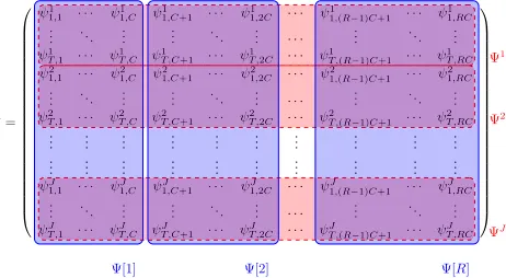
In this first approach, we provide the position of the tar-get by estimating the row and the column which identify the cell occupied in the grid. More precisely, we consider the signature map exactly as defined in (3), but we look at it organized in blocks according to the rows of the discretization grid:

where z ∈ RTJ×1 is the acquired vector in the runtime phase,b2,0= |{i∈ {1,. . .,N}:b[i]>0}|. Ifbis the solution of (6), then the indexˆrsuch thatb[ˆr]=0 is the row occupied by the device.

Then, reorganizing the columns in, we can write it in blocks according to the columns of the grid, i.e.

= [ 1] ,[ 2] ,. . .,[C]

where each block [c]=

[c](1),[c](2),. . .,[c]

(r),. . .,[c](R)

contains thecth column of the previous

Rblocks:

e.g.,[c](r)=[r](c)is thecth column of therth block of.

The estimation of the column cˆ is provided by the solution of

min

b∈Rnz−b2 s. t.b2,0≤k (7)

Thus, the estimated position is given byx=C(ˆr−1)+ ˆc, crossing the estimated rowrˆand columncˆ, as shown in Fig. 3.

Fig. 3Graphical representation of the crossing approach

3.3 Hierarchical approach

In this approach, we refine the spatial sparsity methods by grouping the cells and proposing a hierarchical search of the device position.

The idea is as follows. In the training phase, some adja-cent cells, which form a partition of the ground floor, are grouped into N macroblocks. The dictionary is then rearranged accordingly. For example, let us consider a 6×8 grid andN = 12 groups composed by 2×2 blocks of adjacent cells as shown in Fig. 4.

The matrix is then rearranged to form a new dictio-nary, denoted by

=[ 1] ,[ 2] ,. . .,[N].

Specifically,has the following structure:

where the different colors represent different blocks, com-posed by the cells indicated in Fig. 4. We also rear-range x ∈ RD into a concatenation of N blocks x =

(x[ 1],x[ 2],. . .,x[N]).

In the runtime phase, first, the macroblock occupied by the device is estimated by solving the optimization problem

minz−x2 s. t.x2,0≤k (8)

where x2,0 = |{i ∈ {1,. . .,N} : x[i]2 > 0}|. Sec-ond, ifx is the solution to (8) and is the index such that x[]= 0, the cell occupied by the device in the

selected macroblock is estimated by solving (5), reducing the dictionary to the columns of[].

This approach can be extended to multiple stages and to multiple devices to be localized.

3.4 Hierarchical approach with spatial averages

We now propose an extension of the hierarchical approach. It also operates in two consecutive steps, requir-ing a new signature map, where each block[n] is com-puted taking the mean in the cells constituting the block:

[n]= 1 Ln

Ln

l=1

ψS[n](l) ∈RTJ,

whereLnis the number of cells constituting thenth block andψ_S[n](l)is the column ofindexed byS[n](l)that is thelth component of the subsetS of indices of the cells constituting thenth block.

Referring to Fig. 4, S[ 1]= {1, 2, 9, 10}, S[ 2]= {2, 3, 11, 12}, and so on, are the subsets of indices rep-resenting each block. Thus, for instance, the first block, which is the red-colored one, is computed taking the average of the first, the second, the ninth and the tenth columns of, as defined in (3).

Specifically

This approach is motivated by the fact that averag-ing RSS measurements minimizes the mean square error (MSE) of the RSS values measured in different points. Moreover, if the distance among the reference points is

not too large, compared to the environment dimension, the averaging process is approximately equivalent to take the RSS from the centroid of the reference points. For instance, if we consider four adjacent cells in a macroblock 2×2, the averaging process provides an approximation of the RSS in the middle of the macroblock. Thus, this could be interpreted as a new discretization with bigger cells.

Then, we find the occupied blockˆιby solving (5), and finally we can find the occupied position by solving (5) using the selected block[ˆι]. In all previous approaches, the recovery of the occupied position is computed via Orthogonal Matching Pursuit (OMP) algorithm [21]. We choose OMP instead of a convex optimization routine, such as the interior point or the simplex method [22], since it is computationally more efficient.

4 Hardware implementation and model validation

Before presenting numerical and experimental results, we provide the specifications about the hardware and the software used for the experiments as well as some tests that we performed in order to validate our model.

4.1 Boards and software description

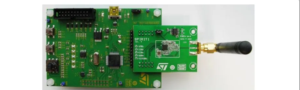
The experiments have been carried out using SPIRIT1-based evaluation boards [23] produced by ST Microelec-tronics (see Fig. 5). The SPIRIT1 is a radio frequency transceiver optimized for low-power operations [24].

This device is designed to operate both in the license-free ISM and SRD frequency bands at 169, 315, 433, 868, and 915 MHz, and can support different modulation schemes. The experiments reported in this paper have been carried out using the 915-MHz band. The SPIRIT1 transceiver provides digital output of the RSS for the last received packet or for the last sequence of received sym-bols. This sensed value is used by each base station to provide the RSS information of the packets received by the device to be localized.

The firmware running on the devices has been devel-oped starting from the Thingsquare [25] open source code, taking advantage of its Contiki operating system [26] core for the programming model and for the net-working support. The experimental results have been col-lected using a set of SPIRIT1-based boards, connected by means of a 6LoWPAN network [27]. A usb-dongle device connected to a laptop has been used to provide the Bor-der Router functionalities to the wireless sensor network (WSN).

4.2 RSS trend and model validation

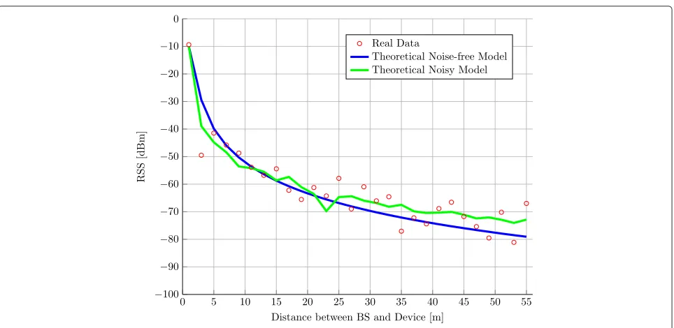
Some experiments have been carried out to evaluate the profile of sensed RSS versus the distance from the receiv-ing device.

We employ two boards, one serving as a base station and the other as the device sending messages to the base station. We start with the two boards next to each other, then we separate them gradually for about 60 m, taking measurements every 2 m, in order to compare these sam-ples with the theoretical model (1). The result is shown in Fig. 6: at each step, we take the average of 20 sam-ples (red circles). Both the noise-free and the noisy model (blue and green curves, respectively) follow the trend of the real sample. The noisy trend is obtained adding Gaus-sian noise to the noise-free model with standard deviation σcomputed from the samples (σ∈[ 0.2, 5.5]).

Another test to validate the considered model is carried out in an outdoor area of size 20×9 m2where we placed six BSs inside the grid. We choose quadrangular cells with a 180-cm-long side. In Fig. 7, we show the trend of the

RSS at a BS, which is located in the ninth row and the sec-ond column. In the first two images, we can see the RSS trend on the ninth row and the second column, respec-tively, while in the second two we display a color-map of the whole area. The RSS value is higher in the neighbor-hood of the BS and decreases with the distance both in the real experiments and in the ideal case.

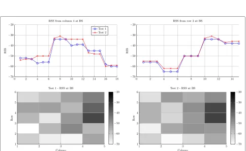
Moreover, in order to check if the trend is more or less constant over time, we take twice the RSS values in a 15× 12.5 m2indoor area at a BS located in the third row and the fourth column. The result of this experiment is shown in Fig. 8: both the trend on a line in the third row and in the fourth column of the grid and the trend on the whole grid are almost the same for both the experiments tested. We can notice that the highest RSS values are in correspondence of the BS and then they decrease with distance.

Finally, in order to validate the choice of SPIRIT1 board, we try also a similar experiment in an indoor area with another kind of board: we test MBxxx [28], a platform based on STM32W with 2.4 GHz, IEEE 802.15.4-compliant transceiver, working with Contiki-OS [26] as well. In this case, as we can see in Fig. 9, the RSS values obtained at a BS located in the fifth row and first column are less stable than the one we obtained with SPIRIT1 boards: as a matter of fact, there are several peaks and unexpected oscillations. This is due to the different trans-mitting frequency: for the SPIRIT1, we use a 915 MHz band, so operating in the sub-GHz band, while for the MBxxx it is 2.4 GHz, which is more noisy since it is the frequency of many other signals (e.g., Wi-Fi). Moreover,

Fig. 7Comparison between RSS trend on a rectangular outdoor area in a simulated case and using SPIRIT1 boards: thetopgraphics represent the RSS trend at a single BS obtained from the column and row the BS occupies; thebottomones, instead, give the RSS map of the whole area at that BS for two different tests

Fig. 9RSS trend on a rectangular indoor area with MBxxx boards: thetopgraphics represent the RSS trend at a single BS obtained from the column and row the BS occupies; thebottomones, instead, give the RSS map of the whole area at that BS for two different tests

a lower frequency brings a longer wavelength, reduc-ing thus the interferences of physical obstacles such as walls.

5 Simulations

In this section, we present the results of some numeri-cal simulations to test our algorithms, comparing them to classical fingerprinting-based algorithms (i.e., WkNN [17]) and to sparse methods [9].

5.1 Classical fingerprinting-based methods

Classical methods are mainly based on nearest neighbor (NN; [17]) procedures, that search for the RP that is the nearest to z. These are widely known clustering meth-ods that can be efficiently applied for fingerprinting-based localization.

Different variations are known, such as k-nearest neighbor (kNN; [17]), and weighted k-nearest neighbor (WkNN; [17]).

The basic idea of NN-based methods is to estimate the position as the weighted mean

ˆ

x= D

i=1 wi D

h=1wh

ξi, (9)

where w = (w1,. . .,wD) are weights, computed in different ways in the different algorithm versions. More precisely, let us define the distances

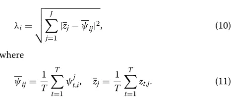
λi=

J

j=1

|zj−ψij|2, (10)

where

ψij= 1 T

T

t=1 ψj

t,i, zj= 1 T

T

t=1

zt,j. (11)

We now define a permutation (i1,i2,. . .,iD) of the sequence(1, 2,. . .,D)such thatλi1 < λi2 < . . . λiD. Then the weighting coefficientsware chosen as in Table 1: in the classical NN we consider only the closest RP putting wi1 =1 and 0 elsewhere; inkNN thekclosest RPs are con-sidered, while in WkNN thekclosest RPs are considered with a weight depending on the distances.

Table 1Weights for deterministic methods based on NN

wi1 wi2 . . . wik wik+1 . . . wiD

NN 1 0 . . . 0 0 . . . 0

kNN 1 1 . . . 1 0 . . . 0

5.2 Results

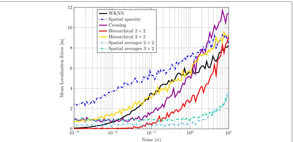
For our simulations, we set an area of 30 × 15 m, on which we build a 12 × 6 grid, with 250-cm-side quad-rangular cells. We deploy J = 8 BSs randomly in the grid, and at each BS we took T = 5 measurements. The signature map is built in a noise free case, follow-ing the model (1), where we set Pt − PL = −50 and n=2.5. Then, for the runtime phase, we generate the real-time measurements using 100 different values of noise (σ) and for each value of σ we have performed 200 experiments.

The results are shown in Fig. 10. Spatial averages meth-ods with blocks of 2×2 cells (lightblue line) turns out to perform best overall and only the hierarchical approach with 2 ×2 block-cells (red line) outperforms it in case of low noise (untilσ < 0.1) since it recovers the exact position almost every time. On the other hand, in case of high noise, spatial averages with 3×2 cells (green line) reaches performance as good as the best one: a mean localization error of 2.5 m means that the average error of 200 experiments is of just one cell. Also our other proposed algorithm based on block-sparsity (crossing approach, violet line) performs close to spatial averages approaches in case of low noise and only for high values ofσ it behaves worse than the spatial sparsity method [9] and the WkNN [17] (blue and black lines, respectively). Finally, with 3×2 cells hierarchical method (yellow line), we incur a mean localization error that is always higher than, or at most the same as, WkNN, but our method is better than spatial sparsity, except for very high noise cases.

5.3 Dictionary design via block-coherence

The block-coherence μB of a dictionary measures the similarity between dictionary elements belonging to dif-ferent blocks, and is defined as

μB():= 1 Tmaxi=j ρ

[i][j],

whereρ [i][j]is the spectral norm of the matrix [i][j]. Conversely, thesub-coherenceis a measure of the correlation of the atoms belonging to the same block, and is defined as

ν():=max i minj=h

θ[i]_j θ[i]h

,

where θj[i] denotes the jth column of the ith block. Theorem 3 in [14] provides a sufficient condition for suc-cessful recovery in absence of noise. More precisely, let x ∈RLW be a blockk-sparse vector (i.e.,x2,0 ≤k) and y=x, where∈RN×LW. If the following inequality is satisfied

kL< 1 2

1 μB()+

L−(L−1) ν() μB()

, (12)

thenxcan be exactly recovered fromy. In practice, this condition requires a small correlation between the atoms belonging to the same block (i.e., a small value ofν()), and a small correlation between the different blocks (i.e., a small value ofμB()).

We perform a Monte Carlo simulation (over 104runs) in order to estimate the probability that a dictionary verifies the block-coherence condition in (12). We remark that the block coherence condition for exact reconstruction holds only in the noise-free case, and no guarantees are given for the noisy case. However, we expect the estimation in (8) to be robust against bounded noise (see [14]): small perturbations in the observations should cause small perturbations in the reconstruction. We build exploiting the RSS model described in Section 2, and we compute a new dictio-nary obtained by reorganizing the columns of the orig-inal matrix , as described in Section 3. We choose several partitions of the ground floor, corresponding to different choices of the block size. For each of these choices, we evaluated the condition in (12). The estimated probability for our block-based approach is reported in Table 2.

For this test, we consider the same settings as in Section 5. We builtexploiting the RSS model described in Section 2, and for each localization approach, we compute a new signature map obtained by reorganizing the columns of the original matrix , as described in Section 3.

In the hierarchical approach, we choose several par-titions of the ground floor, corresponding to different choices of the block size. The estimated probability for the hierarchical approach is summarized in Table 2.

We observe that the best probability is obtained for blocks of size 2×2. This happens because the value of the sub-coherenceνincreases as the block size increases; therefore, the best value ofν is reached when the block size is considered the smallest.

For the crossing approach, instead, the estimated prob-ability is equal to zero. This happens because the block-coherence of the matrix is large, since the blocks of

corresponding to adjacent rows or columns are very similar, thus highly correlated.

Finally, for the hierarchical approach with spatial aver-ages, we consider the same block sizes as in case

Table 2Estimated probabilities for to satisfy sufficient condition (12) for hierarchical approach by changing the size of blocks

of the hierarchical approach. In this case, the esti-mated probabilities are always 1. This is not surpris-ing, because in this case the blocks of matrix have size 1, therefore condition (12) is satisfied if the matrix has a full column rank. This occurs with very high probability.

6 On-field tests

In this section, we show the results of some real experiments, performed in different indoor and outdoor scenarios.

6.1 Outdoor experiments

First of all, we consider an outdoor scenario, where we have less obstacles than in an indoor one, in order to limit the effect of noise to just the interferences from other signals.

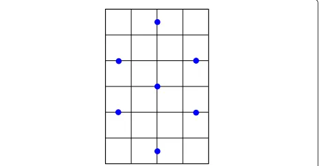
We choose a 6×4 grid with 3-m-side cells in a 18× 12 m open air area. We place allJ=7 BSs, six around the grid and one in the middle, as shown in Fig. 11. At each BS, we tookT =3 measurements both in the training and in runtime phase.

The results are shown in Fig. 12, where we illustrate the cumulative distribution function (CDF) curve with respect to the localization error, which is defined as the probability that the localization error of a single exper-iment X will be found to have a value less than or equal tox:

CDF(x)=P(X≤x).

On a sample of 48 experiments, we obtain that in the 65 % of cases the spatial averages approach (lightblue line) localizes exactly our device, while for more than the 85 %, we have a localization error lower than 3 m, which means we have localized the device at most in an adjacent

Fig. 12Comparison of cumulative distribution functions for different approaches in an outdoor case: a localization error of 0 m corresponds to the exact localization of the device, 3 m means that we localized it in an adjacent cell, 4_·24 m in a diagonal cell, and so on

cell and this can be however considered a success. This approach, as well as the other based on block-sparsity, outperforms all the other approaches considered in this paper: as a matter of fact, about 55 % of the experiments give the exact position for the crossing approach (vio-let line) and the other hierarchical ones (red, vio(vio-let and yellow lines), while the one based on spatial sparsity [9] (blue line) and the WkNN (black line) recovers the cor-rect cell just 30 and 10 % of the times, respectively. We can notice that spatial averages methods increase per-formance of respective hierarchical approaches, and that 2 × 2 blocks are better than 3× 2, as expected from Table 2.

6.2 Indoor experiments

Then, we move into indoor environments, where we expect the localization accuracy to decrease a little due to the higher noise effect given by walls and furniture near the device to be localized and the BSs.

We have considered two different setups. Setup 1: small indoor scenario

Since localization is relevant in smart building contexts, we have tested our algorithms in a household scenario.

In Fig. 13, we can see the house plan with the walls dividing the rooms emphasized by dark red thicker lines. In each room, we considered four cells and deployed all J = 7 BSs (blue dots) in the middle, except for hallway and bathrooms. At each BS, we have takenT =

3 measurements both in the training and in runtime phase.

We run 60 experiments and, as depicted in Fig. 14, the hierarchical algorithm (red line) presents the best perfor-mance, with 2×2 blocks that correspond to the rooms size and 2×1 blocks for the hallway. As expected, the per-formance is worse than in the outdoor scenario due to the presence of walls and furniture that affects the RSS mea-surements; however, spatial averages with the same block configuration and crossing approaches (lightblue and vio-let lines, respectively) recover the exact position between

Fig. 14Comparison of cumulative distribution functions for different approaches in a home scenario: a localization error of 0 m corresponds to the exact localization of the device, 2_·5 m means that we localized it in an adjacent cell, 3_·53 m in a diagonal cell, and so on

50 and 60 % of the experiments, while in the literature [9] (blue line) and [17] (black line) the percentage of suc-cess is about 30 and below 10 %, respectively. Moreover 3×2 blocks approaches, instead, recover the exact posi-tion only in 35 % of the experiments. This is because the blocks have been built overlapping them in the hallway. However, in 80 % of the experiments, all our approaches localize the device in the right room, even if it could be in a wrong cell.

Setup 2: wide indoor scenario

The second indoor scenario considered is the aisle of a university institute, which presents wider rooms with respect to a household scenario. We change also the geometry: we build a 12 × 2 grid with 180-cm-side cells, where we deploy J = 6 BSs (blue dots) on a side of the aisle, as shown in Fig. 15. This configura-tion is more convenient since if we had displaced the BSs along the mid-line, the RSS values read on the left-hand side would have been exactly the same as the one read on the right-hand side. At each BS, we took T = 3 measurements both in the training and in runtime phase.

We run 24 experiments and, as we can see in Fig. 16, the CDF curves’ trend shows that the best algorithms are the hierarchical and the spatial averages approaches with 2×2 blocks (red and lightblue lines, respectively), which give an exact localization of the device between 45 and 50 % of the experiments, or localize it at most in the adjacent one in 80 % of the times. Our other algorithms based on block-sparsity (violet, yellow, and green lines),

instead, are similar to each other, localizing exactly the device in 30 % of the experiments and approaching 80 % if we consider as success even neighboring diagonal cells. Moreover, also in this scenario, all our algorithms out-perform [9] and [17] (blue and black lines, respectively), which localize exactly the device in less than 20 % of the experiments.

Fig. 16Comparison of cumulative distribution functions for different approaches in the university institute aisle: a localization error of 0 m corresponds to the exact localization of the device, 1_·8 m means that we localized it in an adjacent cell, 2_·5 m in a diagonal cell, and so on

7 Conclusions

In this paper, we have introduced new methodologies for RSS-fingerprinting localization in wireless sensor net-works, based on block-sparsity, and we have proved that they perform better than the state-of-the-art techniques through several numerical simulations and real experi-ments. In particular, we have done tests deploying sensors in different indoor and outdoor scenarios.

As in [9], our study arises from the observation that localization of one or few devices can be interpreted as reconstruction of a sparse signal. Our specific contribu-tion improves the results in this framework using block-sparsity, which can be assumed when very few devices have to be localized (which is the most common localiza-tion setting).

Recent mathematical results on block-sparsity provide analytic conditions for signal reconstruction, which have been discussed to support our experimental results.

We also describe a real-world implementation of a sys-tem running for both training and runtime phases: once the localization parameters and the blocks have been set, a device sends messages to base stations, which compute the RSS values and send them to a central unit, where a Java server collects them and runs hierarchical algorithm and outputs the estimate of the device’s position.

Many important aspects that have not been dealt in this work will be investigated in our future research. In par-ticular, we will focus on distributed localization, in which the device is not localized by a central unit that collects and processes the data acquired from the sensor network,

but by the network itself. This raises challenging problems in terms of computational capabilities and transmissions, but would be an extremely appealing feature for all those applications where the network is large and a central unit is inconvenient.

Competing interests

The authors declare that they have no competing interests.

Acknowledgements

This work has received funding from the European Research Council under the European Community’s Seventh Framework Programme (FP7/2007-2013)/ ERC Grant agreement number 279848.

Author details

1_{Department of Electronics and Telecommunications (DET), Politecnico di}

Torino, Corso Duca degli Abruzzi, 24, 10129 Torino, Italy.2_{Department of}

Electronics, Information Science and Bioengineering (DEIB), Politecnico di Milano, Via Ponzio, 34/5, 20133 Milano, Italy.3_{Advanced System Technology,}

STMicroelectronics, Via C. Olivetti 2, 20864 Agrate Brianza, Italy.

Received: 31 October 2014 Accepted: 5 June 2015

References

1. Y Liu, Z Yang, X Wang, L Jian, Location, localization, and localizability. J. Comput. Sci. Technol.25(2), 274–297 (2010)

2. Y Gwon, R Jain, T Kawahara, inProc. of IEEE INFOCOM 24th Annual Joint Conference of the IEEE Computer and Communications Societies. Robust indoor location estimation of stationary and mobile users, vol. 2 (Hong Kong, China, 2004), pp. 1032–1043

3. H Liu, H Darabi, P Banerjee, J Liu, Survey of wireless indoor positioning techniques and systems. IEEE Trans. Syst. Man Cybern. Syst. Part C: Appl.

Rev.37(6), 1067–1080 (2007)

5. A Boukerche, HAB Oliveira, EF Nakamura, AAF Loureiro, Localization systems for wireless sensor networks. IEEE Wireless Commun. 14(6), 6–12 (2007)

6. J Wang, RK Ghosh, SK Das, A survey on sensor localization. J. Control Theory Appl.8(1), 2–11 (2010)

7. Z Farid, R Nordin, M Ismail, Recent advances in wireless indoor localization techniques and system. J. Comput. Netw. Commun.2013, 1–12 (2013) 8. VK Jain, S Tapaswi, A Shukla, Performance analysis of received signal

strength fingerprinting based distributed location estimation system for indoor wlan. Wirel. Pers. Commun.70(1), 113–127 (2013)

9. S Nikitaki, P Tsakalides, inAsilomar Conference on Signals, Systems and Computers. Localization in wireless networks via spatial sparsity (Asilomar, Pacific Grove, CA, US, 2010), pp. 236–239

10. S Nikitaki, P Tsakalides, inIEEE 19th European Signal Processing Conference, 2011. Localization in wireless networks based on jointly compressed sensing (Barcelona, Spain, 2011), pp. 1809–1813

11. S Nikitaki, P Tsakalides, inProc. of 7th ACM Workshop on Performance Monitoring and Measurement of Heterogeneous Wireless and Wired Networks. Decentralized indoor wireless localization using compressed sensing of signal-strength fingerprints (Paphos, Cyprus, 2012), pp. 37–44 12. EJ Candès, MB Wakin, An introduction to compressive sampling. IEEE

Signal Process. Mag.25(2), 21–30 (2008)

13. YC Eldar, M Mishali, Robust recovery of signals from a structured union of subspaces. IEEE Trans. Inf. Theory.55(11), 5302–5316 (2009)

14. YC Eldar, P Kuppinger, H Bolcskei, Block-sparse signals: Uncertainty relations and efficient recovery. IEEE Trans. Signal Process.58(6), 3042–3054 (2010)

15. C Feng, WSA Au, S Valaee, Z Tan, Received-signal-strength-based indoor positioning using compressive sensing. IEEE Trans. Mobile Comput. 11(12), 1983–1993 (2012)

16. A Bay, P Fragneto, M Grella, SM Fosson, C Ravazzi, E Magli, in15th International Workshop on Multimedia Signal Processing. Sparsity-based indoor localization in wireless sensor networks (Pula (Sardinia), Italy, 2013) 17. B Li, J Salter, AG Dempster, C Rizos, inProc. of 1st IEEE International

Conference on Wireless Broadband and Ultra Wideband Communications. Indoor positioning techniques based on wireless LAN (Sidney, Australia, 2006)

18. D Madigan, E Einahrawy, RP Martin, W-H Ju, P Krishnan, A Krishnakumar, in Proc. of IEEE INFOCOM 2005, 24th Annual Joint Conference of the IEEE Computer and Communications Societies. Bayesian indoor positioning systems, vol. 2 (Miami, FL, US, 2005), pp. 1217–1227

19. EJ Candès, The restricted isometry property and its implications for compressed sensing. Comptes Rendus Mathematique.346(9), 589–592 (2008)

20. R Baraniuk, M Davenport, R DeVore, M Wakin, A simple proof of the restricted isometry property for random matrices. Constr. Approx.28(3), 253–263 (2008)

21. JA Tropp, AC Gilbert, Signal recovery from random measurements via orthogonal matching pursuit. IEEE Trans. Inf. Theory.53(12), 4655–4666 (2007)

22. S Boyd, L Vandenberghe,Convex Optimization. (Cambridge university press, Cambridge, UK, 2004)

23. STMicroelectronics, SPIRIT1 Low Data Rate, Low Power Sub 1GHz Transceiver. http://www.st.com/web/catalog/sense_power/FM1968/ CL1976/SC1845/PF253167

24. STMicroelectronics, STEVAL-IKR002V5 SPIRIT1 Low Data Rate Transceiver 915 MHz Full Kit. http://www.st.com/web/en/catalog/tools/PF259026 25. Thingsquare, Homepage. http://thingsquare.com/

26. Contiki, The Open Source OS for the Internet of Things. http://www. contiki-os.org/

27. 6LoWPAN, Proposed Standard. http://tools.ietf.org/html/rfc4944 28. STMicroelectronics, STM32W-EXT Extension boards for evaluation kit for

STM32 Wireless devices. http://www.st.com/web/en/catalog/tools/ PF247100

Submit your manuscript to a

journal and benefi t from:

7Convenient online submission

7 Rigorous peer review

7Immediate publication on acceptance

7 Open access: articles freely available online 7High visibility within the fi eld

7 Retaining the copyright to your article