Partial Interference and Its Performance Impact on Wireless Multiple Access Networks

(1)

Volume 2010, Article ID 735083,20pages doi:10.1155/2010/735083

Research Article

Partial Interference and Its Performance Impact on

Wireless Multiple Access Networks

Ka-Hung Hui,

1

_{Wing Cheong Lau,}

2

_{and Onching Yue}

2

1_{Department of Electrical Engineering and Computer Science, Northwestern University, Evanston, IL 60208, USA} 2_{Department of Information Engineering, The Chinese University of Hong Kong, Shatin, Hong Kong}

Correspondence should be addressed to Wing Cheong Lau,[email protected]

Received 12 February 2010; Revised 9 July 2010; Accepted 12 August 2010

Academic Editor: Kwan L. Yeung

Copyright © 2010 Ka-Hung Hui et al. This is an open access article distributed under the Creative Commons Attribution License, which permits unrestricted use, distribution, and reproduction in any medium, provided the original work is properly cited.

To determine the capacity ofwireless multiple access networks,the interference among the wireless links must be accurately modeled. In this paper, we formalize the notion of the partial interference phenomenon observed in many recent wireless measurement studies and establish analytical models with tractable solutions for various types of wireless multiple access networks. In particular, we characterize the stability region of IEEE 802.11 networks under partial interference with two potentially unsaturated links numerically. We also provide a closed-form solution for the stability region of slotted ALOHA networks under partial interference with two potentially unsaturated links and obtain a partial characterization of the boundary of the stability region for the general M-link case. Finally, we derive a closed-form approximated solution for the stability region for general M-link slotted ALOHA system under partial interference effects. Based on our results, we demonstrate that it is important to model the partial interference effects while analyzing wireless multiple access networks. This is because such considerations can result in not only significant quantitative differences in the predicted system capacity but also fundamental qualitative changes in the shape of the stability region of the systems.

1. Introduction

In a wireless network, all stations communicate with each other through wireless links. A fundamental diﬀerence between a wireless network and its wired counterpart is that wireless links may interfere with each other, resulting in performance degradation. Therefore in the study of wireless networks, one important performance measure is the capacity of the network when the eﬀects of interlink interference are considered.

In establishing the capacity of a wireless network, we have to predict whether the wireless links interfere with each other. Two most common interference models in the wireless networking literature, namely, for example, protocol model and physical model [1], were proposed to predict whether transmissions in a wireless network are successful. In these interference models, one key assumption is that interference is abinary phenomenon, that is, either the links mutually interfere with each other to result in total loss of throughput of a target link, or there is no

(2)

call this phenomenonpartial interference. From the physical layer implementation perspective, the partial interference phenomenon can be viewed as a consequence/manifestation of the probabilistic nature of signal decoding in the receiver, its interaction with the well-known capture eﬀect [10, 11], and the specific implementation of the frame reception and capture algorithms in individual chipsets [12].

While the phenomenon of partial interference in wireless networks has been widely observed as mentioned above, its incorporation in the performance modeling of such networks is still in its infancy. Most of the eﬀorts in this direction so far ([2, 7, 12, 13]) have been limited to the characterization of the nonbinary transitional region in the PRR-versus-SINR curve based on measurement data [7,12,

13] or some analytical means [2, 14]. However, once the PRR-versus-SINR curve is obtained, they only resort to simulations to evaluate the eﬀects of partial interference on the system performance.

In this paper, our focus is to develop analytical mod-els with tractable solutions for various types of wireless multiple access networks which can accurately capture the performance impact of partial interference. Via analytical and numerical results throughout this paper, we demonstrate that it is important to model the partial interference eﬀects while analyzing wireless multiple access networks. This is because such considerations can result in not only significant quantitative diﬀerences in the predicted system capacity but also fundamental qualitative changes in the shape of the stability region of the systems (e.g., from a concave to a convex region).

To quantify the impact of interference on multiple access networks, we propose an analytical framework to characterize partial interference for two representative types of multiple access wireless networks, namely, the IEEE 802.11 Wireless LANs and the classical slotted ALOHA networks. For IEEE 802.11 Wireless LANs, we extend the single-channel Markov model in [15] to take into account theunsaturated traﬃc conditions, the SINR attained at the receivers, and the modulation scheme employed. These modifications result in a partial interference region, which cannot be captured by the binary interference models used in previous works. We also find out the stability (admissible) region of IEEE 802.11 networks with two interfering, potentiallyunsaturated links numerically. For slotted ALOHA networks, we extend the model in [16] to derive the exact stability region of slotted ALOHA with two links while considering partial interference. We show that as the link separation increases, the stability region obtained expandsgraduallyunder partial interference, as in the case of 802.11.

Despite the simplicity of slotted ALOHA, characterizing its exact stability region with unsaturatedlinks is extremely diﬃcult and has remained to be a key open problem for decades when there are more than two, potentially unsatu-rated links in the system [16–23]. However, by extending the FRASA (Feedback Retransmission Approximation for Slotted ALOHA) approach [24] to model the partial interference eﬀects, we obtain aclosed-formapproximation for the exact stability region foranynumber of links.

In summary, this paper has made the following contribu-tions.

(1) After reviewing related work inSection 2, we formal-ize the notion of partial interference inSection 3and then demonstrate its significant performance impact on different types of wireless networks via vari-ous examples and their analytical/numerical results throughout the rest of the paper. As an illustration, we show in Section 4 that, by considering partial interference effects while scheduling traffic in a wireless network of regular topology, the gain in network capacity across unit cutcan be as high as 67%. (2) In Section 5, we establish a model to analyze the effects of partial interference on the throughput of IEEE 802.11 networks with unsaturatedlinks. Our approach enables one to compute numerically the stability region of any 2-link 802.11 system under unsaturatedtraffic conditions.

(3) In Section 6, we investigate the eﬀects of partial interference on the capacity of a slotted ALOHA system with unsaturated links by (i) establishing the exact stability region in closed-form for the 2-link case and (ii) providing a closed-form, partial characterization of the stability region of the general M-link case.

(4) InSection 7, we extend the FRASA approach in [24] to yield a closed-form approximationfor the stability region of the general M-link slotted ALOHA system while considering partial interference effects. The capacity region derived by our approximation and the corresponding simulation results are provided for some sample cases. Again, this is to demonstrate the potential qualitative and quantitative differences in the system capacity region when the effect of partial interference is taken into account. We then conclude the paper inSection 8.

2. Related Work

In [1], two interference models, called the protocol model and thephysical model, were introduced. The protocol model states that a transmission is successful if the corresponding receiver is located inside the transmission range of the trans-mitter, and all other active transmitters are located outside the interference range of the receiver. In the physical model, the transmissions from other transmitters are considered as noise, and a transmission is successful if the SINR attained at the receiver exceeds a certain threshold. Based on these models, the capacities of a multihop wireless network under random and optimal node placement were derived.

(3)

UDP throughputs of an individual link. It was found that the throughputs increased smoothly when the separation between the links increased. The throughputs increased more rapidly as the channel separation between the links increased. Such nonbinary transitional region in the link throughput (or PRR equivalently) as the receiver SINR varies has also been observed by numerous measurement studies including [2–4]. These experimental results all confirmed that the binary assumption in the protocol or physical interference models are not valid in practice.

There has been some analytical work on finding the relationship between the SINR attained at a receiver and the throughput (or PRR equivalently) achieved by the corresponding wireless link. In [14], a methodology for estimating the packet error rate in the aﬀected wireless networkdue to the interference from theinterfering wireless network was presented. The throughput of the aﬀected wireless network was found to increase continuously with the SINR attained at the corresponding receiver, which increased with the separation between the networks. Similarly, [2] derived expressions for the PRR as a function of distance, radio channel parameters, and the modulation/encoding scheme used by the radio. However, they did not provide analytical model on how the PRR function would impact the performance of the corresponding networks.

In [25], the throughput achieved by an M-link IEEE 802.11 network under physical layer capture was derived. While their analysis can be viewed as another case study of the eﬀects of the partial interference over 802.11 networks, their approach only works for the case where all of the links are always saturated, that is, with infinite backlog at the transmitter side. In contrast, the approach proposed in

Section 5of this paper can handle unsaturated links and has provided explicit numerical solutions for the stability region of the 2-link case.

The study of the stability region ofM-user infinite-buﬀer slotted ALOHA was initiated by the study in [17] decades before and is still an ongoing research. The authors in [17] obtained the exact stability region whenM = 2 under the collision channel (i.e., binary interference) model. References [18, 19] used stochastic dominance and derived the same result as in [17] for the case ofM=2.

For general M, there were attempts to find the exact stability region, but there was only limited success. Reference [21] established the boundary of the stability region, but it involves stationary joint queue statistics, which still do not have closed form to date. Instead, many researchers focused on finding bounds on the stability region for general M. Reference [17] obtained separate suﬃcient and necessary conditions for stability. References [18,19] derived tighter bounds on the stability region by using stochastic dominance in diﬀerent ways. Reference [22] introducedinstability rank and used it to improve the bounds on the stability region. However, the bounds in [18,22] are not always applicable. Also, the bounds obtained may not be piecewise linear.

With the advances in multiuser detection, researchers also studied this problem with the multipacket reception (MPR) model. Reference [23] studied this problem in the infinite-user, single-buﬀer, and symmetric MPR case.

Reference [16] considered the problem with finite users and infinite buﬀer. They obtained the boundary for the asymmetric MPR case with two users, and also the inner bound on the stability region for generalM.

3. Partial Interference—Basic Idea

As an illustration to the methodology in [14], assume the underlying modulation scheme used is binary phase shift keying (BPSK). The distance between the transmitter and the receiver and that between the interferer and the receiver aredSanddI meters, respectively. The transmission power of the transmitter and the interferer are PS and PI watts, respectively.

Assuming that the interfering signal can be modeled as additive white Gaussian noise (AWGN) and the background noise can be ignored, we use the two-ray ground reflection model

pl(d)=GTGRh2Th2R

d4 =

C

d4 (1)

to represent the path loss, whereGT andGRare the gain of transmitter and receiver antenna, respectively,hT andhRare the height of transmitter and receiver antenna, respectively, andC = GTGRh2Th2R. The path loss exponent is 4 in this model. We letGT = GR = 1 and hT = hR = 1.5. Then, according to [26], the bit error rate (BER) is given by

1 2erfc

γ, (2)

whereγis the SINR attained at the receiver and is given by

γ=PSpl(dS)

PIpl(dI). (3)

Define the packet-level normalized throughput ρ(γ) to be the ratio of the successful packet reception rate at the receiver when SINR=γto the maximum packet reception rate of the link when BER=0. As such,ρ(γ) is actually the probability of a packet to be received without error when the SINR isγ. Suppose that all packets consist ofLbits and bit errors are identically, independently distributed within each packet. We have

ργ=

1−1 2erfc

γ

L

. (4)

In general,ρ(γ) depends on the BER, which, in turn, is a function of the SINR at the receiver as well as the specific modulation scheme being used. While we use BPSK as an example here, the actual expression forρunder other modu-lation schemes can be readily derived as shown in [2, Table 5].

(4)

with the findings of many empirical studies discussed in

Section 1.

In Figure 1, we also plot the variation of throughput against distance between the interferer and the receiver if the physical model is used. The SINR thresholdγ0for the binary-interference model is set by assuming that whenγ=γ0, the packet error rate is 10−3, that is,

10−3=1−

1−1 2erfc

γ0

L

. (5)

We observe that if the value we assign to γ0 is too large (or the threshold distance is too large), we underestimate the throughput that the links can achieve. On the other hand, if γ0 is too small (or the threshold distance is too small), we introduce excessive interference into the network. In other words, it is diﬃcult to use a single threshold to describe accurately the relationship between interference and throughput of each link in a network.

4. Capacity Gain When Partial

Interference Is Considered

In this section, we demonstrate that there is a gain in system capacity when the eﬀect of partial interference is considered. We consider one variation of the Manhattan network [27], that is, a network consisting of a rectangular grid extending to infinity in both dimensions. The horizontal and vertical separations between neighboring stations are denoted byr andd, respectively.

Under infinite transmitter backlog, the packet-level capacity of each link, that is, the maximum packet reception rate without interference, is denoted byρ0. We assume that diﬀerential binary phase shift keying (DBPSK) is employed and a packet consists ofLbits. We use the two-ray ground reflection model (1) as in previous section to model the path loss. To apply the physical model, we let the SINR thresholdγ0be the case that the packet error rate is, that is, 1−[1−(1/2) exp(−γ0)]L=, where (1/2) exp(−γ) is the bit error rate of DBPSK [26]. We letL=8192 and=10−3, therefore the SINR requirement isγ0=15.23. Assuming that there is no interferer, this SINR requirement is met when the length of a link is smaller than 493 meters.

We use a Cartesian coordinate plane to represent the modified Manhattan network. One station is placed at every point with integral coordinates in the network. Suppose that we schedule flows in the modified Manhattan network from the South to the North using the pattern shown inFigure 2

and its shifted versions. In Figure 2, an arrow is used to represent an active link, where the tail and the head of an arrow denote the transmitter and the receiver of the link, respectively.

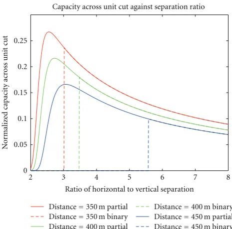
We use thecapacity across unit cut η(μ) as the perfor-mance metric, whereμ = r/dis the ratio of the horizontal separation to the vertical separation. It is a measure on how much traﬃc we can send through a cut in a network on average while physically packing the links towards each other. Consider the SINR attained at the receiver marked with the blue circle, which has the position assigned as the origin in

400 450 500 550 600 650 700 0

0.2 0.4 0.6 0.8 1

Network separation (m)

Relationship between throughput and network separation

Binary Partial

N

o

rm

aliz

ed

thr

oug

hput

Figure1: Throughput degradation and network separation.

−6 −4 −2 0 2 4 6

A sample schedule

Figure2: A scheduling pattern in the modified Manhattan network.

the Cartesian coordinate plane. We assume that all stations transmit with powerP, and each station has a background noise power ofN. The SINR is defined byγ(μ)=S/(N+I(μ)), whereSis the received power from the intended transmitter and I(μ) is the power received from all interferers. The packet-level capacity achieved by each link, that is, the suc-cessful packet reception rate at the receiver, isρ(μ)=ρ0{1− (1/2) exp[−γ(μ)]}L _{under our partial interference model.} On the other hand, under the physical interference model, ρ(μ)=ρ0ifγ(μ)≥γ0andρ(μ)=0 otherwise. AcutCin the network is an infinitely long horizontal line. Let{Tn}n∈Nbe

the set of all active transmitters such thatCintersects the link used byTn. We divideCinto segmentsC(Tn),n∈N, where

C(Tn)= x∈C:x−Tn =min

n_∈_Nx−Tn

(5)

and · is the Euclidean norm. Then the lengthLof the cut occupied by an active transmitter is the length ofC(Tn), and the capacity across unit cut is thereforeη(μ)=fρ(μ)/L, wherefis the fraction of time that a link is active.

In the following we assume thatd = 450 meters, P = 24.5 dBm, andN = −88 dBm. For the schedule inFigure 2, the signal power isS=PC/d4_{. All transmitters in}_{Figure 2}_are located at positions (x, 4y−1), wherexandyare integers. The interference power is

Iμ=

Considering the physical model, if the schedule is allowed to be active, we needμ ≥ μ0 = 5.58, as listed inTable 1 and depicted inFigure 3by the blue dashed line. The value ofμ0is obtained fromγ(μ0)=γ0. Each active transmitter occupies a cut of lengthr=μd, and each link is active for one quarter of a cycle. Therefore, forμ=μ0, the maximum capacity across unit cut under the physical model isρ0/4μ0d=0.0996ρ0bits per second per kilometer.

If we allow partial interference, the active transmitters can be packed more closely. Whenμdecreases, more spatial reuse is allowed. The increase in the density of active transmitters outweighs the degradation in capacity, so there is an increase in the capacity across unit cut. However, ifμ decreases further, interference will be the dominant factor in determining the capacity across unit cut. Therefore, the capacity across unit cut drops, and there exists μopt for the optimal performance under partial interference. This behavior is depicted by the blue solid line inFigure 3. The optimal value of μ under partial interference is μopt = 3.06, and the capacity across unit cut is 0.1661ρ0 bits per second per kilometer. There is a percentage increase of 66.82% in the capacity across unit cut when the eﬀect of partial interference is considered. Similar results are shown in

Table 1andFigure 3ford=350, 400 meters. The percentage increase is larger when the links are longer, but the capacity achieved by each link reduces. We can viewμ0das the carrier sensing range in the modified Manhattan network with the scheduling pattern inFigure 2, as it is the smallest horizontal separation allowed by the physical model. We observe that if the length of the links increases, the carrier sensing range needs to be increased in a larger proportion. Also, this carrier sensing range is much larger than double of the length of the links, which is the usual convention used in defining the relationship between carrier sensing range and transmission range.

5. Partial Interference in 802.11

In this section, we study partial interference in 802.11 networks, the prevalent wireless random access networks.

2 3 4 5 6 7 8

Capacity across unit cut against separation ratio

Ratio of horizontal to vertical separation

Distance=350 m partial Distance=350 m binary Distance=400 m partial

Distance=400 m binary Distance=450 m partial Distance=450 m binary

N

Figure 3: Capacity across unit cut for diﬀerent lengths of links under the physical model (binary interference) and partial interfer-ence.

Table1: Capacity gain in the modified Manhattan network with diﬀerent lengths of links.

d μ0 η(μ0) μopt η(μopt) % increase

350 3.02 0.2365ρ0 2.55 0.2671ρ0 12.93%

400 3.48 0.1796ρ0 2.73 0.2163ρ0 20.45%

450 5.58 0.0996ρ0 3.06 0.1661ρ0 66.82%

We present an analytical framework to characterize partial interference in a single-channel wireless network under unsaturated traﬃc conditions, which uses 802.11b with basic access scheme and DBPSK. We show that there is a partial interference region, in which the throughput of each link increases continuously with the separation between the links in the network. As a first attempt to relate the capacity-finding problem in wireless random access networks to the stability region of such networks, we derive the admissible (stability) region of an 802.11 network with two potentially unsaturated links numerically.

5.1. The 802.11 Model. We present our framework to characterize partial interference in a wireless network with random access protocols. In this framework, we derive the transmission probabilities τn and the packet corruption probabilities cn of the links in the network. τn is the probability that a station transmits in a randomly chosen slot, whilecnis the probability that a packet is received with error.

(6)

modulation schemes. In addition, we make the following assumptions.

(i) The network consists of two links (T1,R1) and (T2,R2), whereTnandRndenote the transmitter and the receiver of the links, respectively,n=1, 2. (ii) There are a constant buﬀer nonempty probabilityqn

that the transmission buﬀer ofTnis nonempty and a constantchannel idle probabilityinthatTnsenses the channel to be idle,n=1, 2.

(iii)Tn transmits with power Pn, and the background noise power atRnisNn,n=1, 2.

(iv) Channel defects like shadowing and fading are neglected, and a generic path loss model pl(d) = Cd−α_{is used to model the wireless channel, where}_d_is the propagation distance,αis the path loss exponent, andCis a constant.

(v) The interference from other transmitters plus the receiver background noise is assumed to be Gaussian distributed.

(vi) All bits in a packet must be received correctly for correct reception of the packet.

(vii) The size of an acknowledgement is much smaller than that of the payload, so the bit errors on acknowledgement are negligible.

We follow the approach as in [15], using a discrete-time Markov chain to model the 802.11 Distributed Coordination Function (DCF) and obtain the transmission probability of a station. An ordered pair (j,k) is used to denote the state of the Markov chain, where j represents the backoffstage andk is the current backoffcounter value. In stage j,k is in the range [0,Wj−1], whereWjis the contention window size in stage j.mis the maximum number of backoffstages. However, there are some discrepancies between the model in [15] and the actual behavior of 802.11 DCF. First, the model assumes that a station retransmits indefinitely until the packet is successfully transmitted. This assumption is inconsistent with 802.11 basic access scheme. Also, the model does not account for the unsaturated traffic conditions, which is the scenario appeared in practical situations.

To overcome these limitations, we adopt and modify the Markov chain proposed by [15] to obtain an enhanced model. First, we take into account the limited number of retransmissions in 802.11 as in [28], by restricting the Markov chain to leave the mth backoff stage once the station transmits a packet in that backoff stage. Second, we follow [28] to modify the values of Wj in accordance with the 802.11 MAC and PHY specifications [29], withm corresponding to the first backoffstage using the maximum contention window size

In addition, to handle the unsaturated traﬃc conditions, we follow [30] to augment the Markov chain by introducing new

−1, 0

Figure4: A Markov chain model for 802.11 DCF in unsaturated conditions.

states (−1,k),k ∈ [0,W0−1]. These new states represent the states of being in the post-backoffstage. The post-backoff stage is entered whenever the station has no packets queued in its transmission buffer after a successful transmission. The corresponding Markov chain is depicted inFigure 4.

Let πj,k denote the stationary probability of the state (j,k) in the Markov chain. The transmission probability of a station is given by

τn=π−1,0qnin+

The details of the Markov chain and the derivation of this equation can be found in [31].

The packet corruption probability is calculated according to the modulation scheme used in the PHY layer, the distance between the transmitter and the receiver, and the existence of nearby interferer(s). For a fixed carrier sensing threshold β, we diﬀerentiate into two cases, whether both transmitters can sense the transmission of each other or not.

(7)

The bit error rate attained by (T1,R1) is e(γ1) = (1/2) exp(−γ1), and the packet corruption probability for (T1,R1) is header, the MAC header, and the payload, respectively.

On the other hand, ifT1cannot sense the transmission of T2, that is,P2pl(dT1,T2)≤β, then the SINR atR1depends on

whetherT2is active in transmission or not, that is,

Prγ1=γ

The packet corruption probability is calculated by the average bit error rateE[e(γ1)]

The channel idle probability is defined as follows. IfT1 can sense the transmission ofT2, then T1will consider the channel to be idle wheneverT2is inactive, that is,i1=1−τ2; otherwiseT1always senses the channel to be idle andi1=1.

Suppose that we want to schedule a flow ofλnbits per second on (Tn,Rn) and ρn bits per second is achieved by (Tn,Rn),n=1, 2. We referλnandρnto theoﬀered loadand thecarried load, respectively. We calculateρnby

ρn=τn(1−cn)L

E[Sn]

, (14)

where E[Sn] is the expected length of a slot as seen by (Tn,Rn). Let an be the probability that at least one station is transmitting, and let sn be the probability that there is at least one successful transmission given that at least one station is transmitting. ThenE[Sn]=(1−an)σ+ansn(Ts+ σ) +an(1−sn)(Tc+σ), whereσ,Ts, and Tc are the time spent in an idle slot, a successful transmission, and an unsuccessful transmission, respectively. WhenT1 can sense the transmission of T2, we consider both links to be one system:

Otherwise, we treat both links to be separate systems:

a1=τ1,

s1=1−c1.

(16)

We approximate the packet arrival of (Tn,Rn) to be a Poisson process with rate λn/L,n = 1, 2, and estimate the buﬀer nonempty probability by

qn=1−exp −λn

LE[Sn]

. (17)

In summary, ifT1can sense the transmission ofT2, then we obtain the following set of equations for (T1,R1):

Otherwise, we obtain another set of equations for (T1,R1)

τ1=

Similarly, we can obtain three equations for link (T2,R2). With these six equations we can solve for the variablesτ1, c1, q1,τ2, c2, q2 by Newton’s method [32] and obtain the loadings of these two links by (14).

5.2. Some Analytical Results. We use the two-ray ground reflection model

pl(d)=GTGRh2Th2R

d4 =

C

d4 (20)

(8)

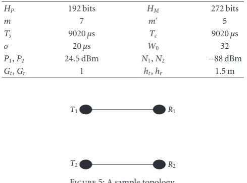
Table2: Parameters used for the analytical results.

HP 192 bits HM 272 bits

m 7 m 5

Ts 9020μs Tc 9020μs

σ 20μs W0 32

P1,P2 24.5 dBm N1,N2 −88 dBm

Gt,Gr 1 ht,hr 1.5 m

T1 R1

T2 R2

Figure5: A sample topology.

In the following we attempt to find the maximum carried loads of each link in various scenarios. One observation from solving the system of equations in Section 5.1 is that the carried load will be smaller than the offered load when the offered load is too large. This corresponds to the instability of 802.11 observed in previous works (e.g., [15]). Therefore, we use binary search to find the maximum carried load under stable conditions. Initially, the search range for the offered load is between 0 and 1 Mbps. We choose the midpoint of the search range to be the offered load and solve the system of equations. If the resultant carried load is the same as the offered load, the offered load can be increased, and the next search range will be the upper half of the original one. Other-wise, the offered load results in instability, and the next search range will be the lower half of the original one. This proce-dure is repeated until the search range is sufficiently small.

We consider a network of two parallel links as shown in

Figure 5, withd andr representing the length of the links and the link separation, respectively. The link separation is defined as the perpendicular distance between the links. We letL=8192 bits,d=450 meters, andβ= −70,−75,−78, −80 dBm to solve for the maximum carried loads and obtain the curves as shown in Figures6(a)–6(d).

Consider the curve corresponding to the carrier sensing threshold of −78 dBm in Figure 6(c), which is a common value used in NS-2 simulation and the practical value used in Orinoco wireless LAN card. The corresponding carrier sensing range is 550 meters, which is in line with the carrier sensing range used in practice. In our model, we assume that carrier sensing works when the separation is within the carrier sensing range and fails otherwise and use two diﬀerent sets of equations to model the system in these situations. Therefore there is an abrupt change in the aggregate throughput when the separation equals the carrier sensing range. If there is no carrier sensing in the system, the aggregate throughput will reduce to zero smoothly when the link separation reduces.

The curve inFigure 6(c)can be divided into three parts according to the link separation r. When r < 550 meters,

both transmitters are in the carrier sensing range of each other. As a result, at most only one transmitter is active at a time. Ifr ≥ 550 meters, the transmitters are unaware of the existence of each other, and they contend for the wireless channel as if there were no interferers nearby. Whenr >800 meters, the separation is so large that there will not be any interference between the links. Whenrlies between 550 and 800 meters, the aggregate throughput of the links increases smoothly asrincreases. We label this range ofras thepartial interference region. The existence of this partial interference region suggests that the interference models proposed by [1] that a single threshold can represent the interference relationship in wireless networks may be overly simplified.

The width of this partial interference region depends on the carrier sensing thresholdβused. Smallerβ, for example, −80 dBm, results in a narrower partial interference region as inFigure 6(d). Simultaneous transmissions are allowed only for the links separated far enough, and the throughput is suppressed significantly. For largerβ, for example,−75 and −70 dBm, morespatial reuseis allowed, and the width of the partial interference region is larger, as shown in Figures6(a)

-6(b). However, excessive interference is introduced for larger β, so there is a reduction in the aggregate throughput.

Besides carrier sensing threshold, the length of the links dalso aﬀects the partial interference region. We reducedto be 400 meters and obtain the results in Figures7(a)–7(d). As shown in Figures7(a)–7(d), the partial interference region becomes narrower for all values of carrier sensing threshold. Also, the aggregate throughput achieved by the links is larger for the same link separation when the links are shortened.

5.3. Admissible (Stability) Region. As an attempt to obtain the capacity of 802.11 networks under partial interference, we compute theadmissible (stability) regionpredicted from our model. The admissible region includes all flow vectors (λ1,λ2) such that if (λ1,λ2) is located inside the admissible region, then a flow ofλncan be allocated on and achieved by (Tn,Rn),n=1, 2. We use the same settings as above and choose the carrier sensing threshold to be−78 dBm. The link separations are chosen to be 500, 600, and 900 meters for illustrative purposes, because they correspond to diﬀerent shapes of the admissible region.Figure 8shows the admis-sible region for these three link separations. The link sepa-ration of 500 meters represents that the links are in mutual interference and the admissible region has a triangular shape. When the links are separated by 900 meters, the links do not interfere with each other, and the admissible region is rect-angular. For the link separation of 600 meters, partial inter-ference exists and the admissible region becomes convex.

(9)

300 400 500 600 700 800 900 0

0.5 1 1.5

2 Aggregate throughput against link separation

Distance betweenT1andT2(m)

A

gg

regat

e

thr

oug

h

put

(Mbps)

CST= −70 dBm

(a)−70 dBm

300 400 500 600 700 800 900

0 0.5 1 1.5 2

Aggregate throughput against link separation

A

gg

regat

e

thr

oug

h

put

(Mbps)

CST= −75 dBm

(b)−75 dBm

300 400 500 600 700 800 900

0 0.5 1 1.5 2

A

gg

regat

e

thr

oug

h

put

(Mbps)

CST= −78 dBm

(c)−78 dBm

300 400 500 600 700 800 900 0

0.5 1 1.5 2

A

gg

regat

e

thr

oug

h

put

(Mbps)

CST= −80 dBm

(d)−80 dBm

Figure6: Aggregate throughput for the topology inFigure 5with length of links=450 meters and various carrier sensing thresholds.

6. Partial Interference in Slotted ALOHA

In order to obtain insights in the stability region of general 802.11 networks, in this section, we study the stability of slotted ALOHA, which is a simpler random access protocol, under the assumptions of finite links and infinite buﬀer.

6.1. The Finite-Link Slotted ALOHA Model. LetM= {n}M n=1 be the set of links in the slotted ALOHA system. Time is slotted. The following assumptions apply to all links n ∈ M. Let Tn and Rn be the transmitter and the receiver of link n, respectively. Tn has an infinite buﬀer. The packet arrival process at Tn is Bernoulli with mean λn and is independent of the arrivals at other transmitters.Tnattempts

a virtual transmission with probability pn, that is, if its buﬀer is nonempty,Tnattempts anactual transmissionwith probability pn; otherwise, Tn always remains silent. Also definep_n=1−pn.

In the system, each time slot is just enough for trans-mission of one packet. Packets are assumed to have equal lengths. We assume that transmission results are independent in each slot. For n ∈ A ⊆ M, letqM_n,A be the probability

(10)

We let Qn(t),t ∈ Nbe the queue length in Tn at the beginning of slottand use anM-dimensional Markov chain QM(t) = (Qn(t))n∈M to represent the queue lengths in all

transmitters. We denote by An(t) the number of packets arrived at Tn in slot t and Dn(t) the number of packets successfully transmitted in slot t by Tn when Qn(t) > 0. ThenQn(t+ 1) = [Qn(t)−Dn(t)]++An(t), where [z]+ = max{0,z}is used to account for the case that there is no packet transmitted whenQn(t) = 0. We use the definition of stability in [16,21,22].

Definition 1. AnM-dimensional stochastic processQM(t) is stable if forx∈NM_{the following holds:}

lim t→ ∞Pr

QM(t)<x=F(x), lim

x→ ∞F(x)=1. (21)

If the following weaker condition holds instead,

lim

x→ ∞lim inft→ ∞ Pr

QM(t)<x=1, (22)

then the process issubstable. The process isunstableif it is neither stable nor substable.

The stability problem of slotted ALOHA we consider here is to determine whether the slotted ALOHA system with the set of links M is stable given the parameters{λn}n∈M and {pn}n∈M. We use the result from [34]. On the assumption

that the arrival and the service processes of a queue are stationary, the queue is stable if the average arrival rate is less than the average service rate, and the queue is unstable if the average arrival rate is larger than the average service rate. We also define the slotted ALOHA system to be stable when all queues in the system are stable.

6.2. Stability Region of 2-Link Slotted ALOHA under Partial Interference. We extend the model in [16] to capture the impact of partial interference on the capacity of a 2-link slotted ALOHA system with potentially unsaturated oﬀered load. For n ∈ M, let Pn and Nn be the transmission power used byTn and the background noise power at Rn, respectively. Assume that the signal propagation follows the path loss model pl(d) = Cd−α_{, where} _d_{is the propagation} distance, αis the path loss exponent, and C is a constant. We let γMn,A be the SINR attained at Rn when{Tn}_n_∈_A is the set of active transmitters. Assume that a packet consists ofLbits. Lete(γ) be thebiterror rate when the SINR isγ. In particular, if DBPSK is used in the physical layer,e(γ)= (1/2) exp(−γ). Under binary interference, we let the SINR thresholdγ0be the case that the packeterror rate is, that is, 1−[1−(1/2) exp(−γ0)]L=. ConsiderM=2. When only T1is active, the SINR attained atR1isγM_1,{1}=P1Cd_T−1α,R1/N1,

and

qM

1,{1}=

⎧ ⎨ ⎩

1, γ1,{1}M ≥γ0,

0, γ1,{1}M < γ0,

(23)

wheredX,Y is the distance betweenXandY. When bothT1 andT2are active, thenγM1,{1,2} =P1CdT−1α,R1/(P2Cd

−α T2,R1+N1)

is the SINR attained atR1, and

qM

1,{1,2}=

⎧ ⎨ ⎩

1, γ1,{1,2}M ≥γ0,

0, γ1,{1,2}M < γ0.

(24)

If we consider partial interference instead, we can calculate qM

n,Aas follows. When onlyT1is active,

qM

1,{1}=

1−eγM1,{1}

_L

. (25)

When bothT1andT2are active,

qM_1,{1,2}=1−eγM1,{1,2}

_L

. (26)

Similarly, we can derive expressions for qM_2,{2} and qM_2,{1,2} under binary and partial interference.

To evaluate the boundary of the stability region for the 2-link slotted ALOHA system, we use stochastic dominance as introduced in [18]. We use SP to represent adominant systemof the original systemS, withP being thepersistent set. The transmitters of the links in this set transmit dummy packets when they decide to transmit but do not have packets queued in their buﬀer. The remaining transmitters behave identically as those in S. We first consider the dominant system S{1}. In this dominant system, the successful trans-mission probability of link 2 is p2p₁qM2,{2} + p2p1qM2,{1,2}. For link 1, the queue in T2 is empty with probability 1−λ2/(p2p₁qM_2,{2}+p2p1qM_2,{1,2}); in this case the successful transmission probability isp1qM1,{1}; otherwise, the successful transmission probability is p1p2qM1,{1}+ p1p2qM1,{1,2}. Hence, the average successful transmission probability of link 1 is

p1qM1,{1}

1− λ2

p2p1qM2,{2}+p2p1qM2,{1,2}

+p1p₂q_1,{1}M +p1p2qM_1,{1,2}

_λ

2

p2p1qM2,{2}+p2p1qM2,{1,2}. (27)

With the following notations,

λ1=p1p2q1,{1}M +p1p2qM1,{1,2},

λ2=p2p1q2,{2}M +p2p1qM2,{1,2},

ΔqM

1,{1},{2}=qM1,{1}−qM1,{1,2}, ΔqM

2,{2},{1}=qM2,{2}−qM2,{1,2},

(28)

the stability region ofS{1}is

λ1< p1qM1,{1}−

λ2p2p1ΔqM_1,{1},{2}

λ2

(11)

300 400 500 600 700 800 900 0

0.5 1 1.5 2

A

gg

regat

e

thr

oug

h

put

(Mbps)

CST= −70 dBm

(a)−70 dBm

300 400 500 600 700 800 900

0 0.5 1 1.5 2

A

gg

regat

e

thr

oug

h

put

(Mbps)

CST= −75 dBm

(b)−75 dBm

300 400 500 600 700 800 900

0 0.5 1 1.5 2

A

gg

regat

e

thr

oug

h

put

(Mbps)

CST= −78 dBm

(c)−78 dBm

300 400 500 600 700 800 900

0 0.5 1 1.5 2

A

gg

regat

e

thr

oug

h

put

(Mbps)

CST= −80 dBm

(d)−80 dBm

Figure7: Aggregate throughput for the topology inFigure 5with length of links=400 meters and various carrier sensing thresholds.

and by symmetry, the stability region ofS{2}is

λ2< p2qM2,{2}−

λ1p1p2ΔqM_2,{2},{1}

λ1

, λ1< λ1. (30)

The union of these two regions constitutes the inner bound on the stability region of the original systemS.

The reason for the union of these two regions to be the outer bound on the stability region follows from the indistinguishability argument [16, 18]. Consider the dominant system S{1}. With a particular initial condition on the length of the queues, if the queue inT1is unstable, it is equivalent to the case that the queue in T1 never empties with nonzero probability. ThenS{1} andSwill be indistinguishable, in the sense that the packets transmitted

fromT1inS{1}are always real packets andSis also unstable. Therefore, the union of the regions defined by (29) and (30) is theexactstability region forM=2.

6.3. Some Illustrations. In this section, we depict the stability region derived in previous section by considering the parallel-link topology inFigure 5. We use the two-ray ground reflection model

pl(d)=GTGRh2Th2R

d4 (31)

to represent the path loss. The values of various parameters are shown inTable 3.

(12)

0 0.2 0.4 0.6 0.8 1

Admissible Region

Throughput of link 1 (Mbps)

Thr

o

ug

hput

of

link

2

(Mbps)

Distance=500 m Distance=600 m Distance=900 m

Figure8: Admissible region for various link separations.

Table3: Parameters used for the analytical results.

P1,P2 24.5 dBm N1,N2 −88 dBm

GT,GR 1 hT,hR 1.5 m

0.001 dT1,R1,dT2,R2 450 m

distance between the links, to obtain the results under binary interference in Figure 9(a). The stability region has only two possible shapes. For the separations of 600, 800, and 1000 meters, the SINR attained at either receiver when both transmitters are active is smaller than the threshold. There-fore the underlying channel follows the collision channel model, and the stability region is nonconvex. When the separation is 1200 meters, the links are separated far enough so that transmissions on both links are independent. The channel can be regarded as the orthogonal channel, and the stability region is convex. Therefore, the threshold in binary interference determines when toswitchbetween the collision channel and the orthogonal channel.

Figure 9(b)shows the corresponding results under par-tial interference. When the link separation is small, the amount of interference is so large that partial interference degenerates to the collision channel. As the link separation increases, the stability region expands gradually and changes from nonconvex to convex. At another extreme, when the links are suﬃciently far apart, partial interference is identical to the orthogonal channel. Therefore, partial interference can be viewed as a generalization of binary interference that it interpolatesthe transition from the collision channel to the orthogonal channel. Notice that the results here are similar to the case in 802.11, therefore our results should be applicable to networks with practical random access protocols like 802.11.

Next, we assume that the links are separated by 800 meters. We let both links transmit with probability p and illustrate the eﬀect of p on the convexity of the stability region under binary interference in Figure 10(a). When p is small, that is, 0.2 and 0.4, the links are too conservative in attempting transmissions. It leads to better channel utilization by adding one more link to the system, and the stability region is convex. On the other hand, whenpis large, that is, 0.6 and 0.8, the links are too aggressive. When one more link is added to the system, it increases contention and hence reduces the loading supported by each link drastically. As a result, the stability region is nonconvex. The convexity of the stability region can therefore be regarded as a measure of the contention level in a network.

Figure 10(b)illustrates the stability region when partial interference is considered instead, under the same settings. Although the SINR attained at a receiver when both transmitters are active is smaller than the threshold, the SINR is large enough to support a sustainable throughput probabilistically. Therefore, it is possible to receive more packets opportunistically under partial interference, thereby increasing the loading supported by each link and allowing the stability region to be convex. If we compare the stability region under binary and partial interference in identical settings, as shown in Figures11(a)–11(d), the stability region under partial interference is always larger than that under binary interference. This implies that by considering partial interference, more combinations of flows on the links can be admitted, and the capacity of a wireless network can be potentially increased.

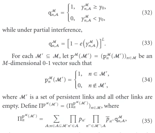
6.4. Partial Characterization of the Stability Region for the M-Link Case. In this section, we give in closed form a partial characterization on the boundary of the stability region of M-link slotted ALOHA under partial interference. First, for

n∈A⊆M,γnM,A=PnCdT−nα,Rn/(

!

n_∈_A_\{_n_}P_nCd_T−α

n,Rn+Nn). Therefore, under binary interference,

qM

n,A=

⎧ ⎨ ⎩

1, γnM,A≥γ0,

0, γnM,A< γ0,

(32)

while under partial interference,

qM

n,A=

1−eγMn,A

L

. (33)

For eachM ⊆M, letpM(M)=(pM_n(M))_n_∈_Mbe an M-dimensional 0-1 vector such that

pM

n (M)=

⎧ ⎨ ⎩

1, n∈M_,

0, _{n /}∈M_, (34)

whereM is a set of persistent links and all other links are empty. DefineΠpM(M₎

=(ΠpnM(M))n∈M, where

ΠpM(M₎

n =

A:n∈A⊆M "

n_∈_A

pn

"

n_∈_M_\_A

p_nqM_n,A, (35)

(13)

0 0.2 0.4 0.6 0.8 1

Loading on link 1

Loading

o

n

link

2

Distance=600 m Distance=800 m

Distance=1000 m Distance=1200 m Stability region of slotted ALOHA under binary interference

(a) Binary interference

0 0.2 0.4 0.6 0.8 1

Loading on link 1

Loading

on

link

2

Distance=600 m Distance=800 m

Distance=1000 m Distance=1200 m Stability region of slotted ALOHA under partial interference

(b) Partial interference

Figure9: Stability region forM=2 with transmission probabilities 0.8 under binary and partial interference.

0 0.2 0.4 0.6 0.8 1

Loading on link 1

Loading

on

link

2

p=0.2

p=0.4

p=0.6

p=0.8

Stability region of slotted ALOHA under binary interference

(a) Binary interference

0 0.2 0.4 0.6 0.8 1

Loading on link 1

Loading

on

link

2

p=0.2

p=0.4

p=0.6

p=0.8

Stability region of slotted ALOHA under partial interference

(b) Partial interference

Figure10: Stability region forM=2 with link separation 800 meters under binary and partial interference.

Theorem 2. All corner points lie on the boundary of the stability region.

Proof. Refer toAppendix A.

By using stochastic dominance and the indistinguishabil-ity argument, we obtain the following theorem.

Theorem 3. LetΠpM(P)_,_ΠpM₍_P_∪_D₎

be two corner points such

thatD = {n} ⊆ M\P. Then the line segment joining these

two points lies on the boundary of the stability region. This line segment represents the case thatP is the set of persistent links while n is the only nonempty nonpersistent link in the system.

Proof. Refer toAppendix B.

(14)

900 meters. Each link transmits with probability 0.6. Other parameters are the same as in Table 3. From Theorem 2, each of the eight 3-dimensional 0-1 vectors corresponds to a corner point shown inFigure 12(b), and their coordinates can be obtained from (35). By Theorem 3, the solid lines in Figure 12(b) are part of the boundary of the stability region. As another example, for M = 2, notice that (29) and (30) are special cases of (B.1). As a direct consequence of our Theorems 2 and 3, the stability region of slotted ALOHA with two links under partial interference is piecewise linear.

7. Stability Region of

the General M-Link Slotted

ALOHA System under

Partial Interference

Theorems2and3cover all cases with zero or one nonempty nonpersistent link in an M-link system, respectively. How-ever, if there are at least two nonempty unsaturated links, the stationary joint queue statistics must be involved in calculating the boundary. Unless we are able to compute the stationary joint queue statistics in closed-form, we are unable to solve the capacity-finding problem, even assuming one of the simplest random access protocol, that is, slotted ALOHA. In fact, the characterization of the exact stability region of a general M-link slotted ALOHA system with nonpersistent links has remained to be a key openproblem for decades

when M > 2 [16–23] even under the simplified binary

interference model.

To overcome the problem caused by the stationary joint queue statistics, we have introduced the FRASA (Feedback Retransmission Approximation for Slotted Aloha) model in [24] to obtain a closed-form approximation for the stability region of a general M-link slotted ALOHA system under binary interference (i.e., simple collision channel) assumptions. We refer the readers to [24, 31] for a detailed description of the FRASA approach. In the following subsection, we extend the model and analysis in [24] to cover the partial interference case. We remark that our results here automatically apply to the binary interference case if we allow qM_n_,_A to be either zero or one only by comparing the corresponding SINR, that is, γnM,A, against a predefined threshold γ0, as illustrated in (32) and (33).

7.1. FRASA under Partial Interference. Assume identical settings as in [24]. There areMlinks in the network, and the set of links is denoted byM = {n}M

n=1. Denote this FRASA system byS. Letp=(pn)n∈Mbe the transmission probability

vector. Define pn =1−pnfor alln∈M. We first consider areduced FRASA system, in which we letM−1 of the links have fixed aggregate arrival rates and the remaining link is assumed with infinite backlog. Taken# ∈ M to be the link with infinite backlog and denote this reduced FRASA system bySn#. Letχnbe the aggregate arrival rate of linkn∈M\{n}# , where χn is between zero and one. Hence, link #nis active with probability pn#, while for n /=#n, link n is active with

Equation (36) is the probability of successful transmission of linkxgiven that linkxis active but link yis not. Equation (37) is the probability of successful transmission of link x given that both linksxandyare active. Equation (38) is the probability of successful transmission of linkxgiven that link xis active. Then the parametric form of the stability region ofSn#will beλn=λn,∀n∈M, where

vector under partial interference.

With this parametric form, we obtain the stability region of FRASA under partial interference as in the following theorem.

Theorem 4. For eachn# ∈ M, one constructs a hypersurface F#n, which is represented byλn=λn,∀n∈M, where

Proof. Refer toAppendix C.

An illustration of the results of Theorem 4 with the topology inFigure 12(a)is given inFigure 13. Figures13(a),

(15)

0 0.2 0.4 0.6 0.8 1

Loading on link 1

Loading

on

link

2

Partial interference Binary interference

Stability region of slotted ALOHA

(a) p1=p2=0.2

0 0.2 0.4 0.6 0.8 1

Loading on link 1

Loading

on

link

2

(b) p1=p2=0.4

0 0.2 0.4 0.6 0.8 1

Loading on link 1

Loading

on

link

2

(c) p1=p2=0.6

0 0.2 0.4 0.6 0.8 1

Loading on link 1

Loading

on

link

2

(d) p1=p2=0.8

Figure11: Stability region forM=2 under binary interference and partial interference with various transmission probabilities.

7.2. Simulation Results. In this subsection, we demonstrate the eﬀects of partial interference on the stability region of the general M-link slotted ALOHA systems by presenting results based on both simulation as well as the FRASA closed-form approximation approach. In particular, we perclosed-form simulations as in [24] to obtain the stability region of slotted ALOHA by considering the ring topology in Figure 12(a). We assume that all links transmit with probability 0.6. For illustrative purpose, we only show the cross-sections of the stability regions. InFigure 14(a), we depict the cross-sections of the stability region by fixing λ2, while in Figure 14(b) the cross-sections of the stability region are obtained by fixing λ1. The solid lines represent the simulation results

(16)

−200 0 200 400 600 800 1000 1200 1400

(a) A sample topology

0 Stability region of slotted ALOHA

(b) Part of the exact boundary

Figure12: Stability region withM=3.

0

(a) F1, boundary of stability region with link 1 infinitely backlogged

0

(b) F2, boundary of stability region with link 2 infinitely backlogged

0

(c) F3, boundary of stability region with link 3 infinitely backlogged

0

(d)R, the whole stability region

Figure13: Stability region of FRASA under partial interference withM=3, transmission probabilities 0.6 and topology inFigure 12(a)by

(17)

0 0.1 0.2 0.3 0.4 0.5 0.6

0 0.1 0.2 0.3 0.4 0.5 0.6 Loading on link 1

Loading

o

n

link

3

Load 2=0S Load 2=0_A Load 2=0.2S

Load 2=0.2A Load 2=0.4S Load 2=0.4A Slices of stability region of slotted ALOHA

(a)λ2fixed, partial interference

0 0.1 0.2 0.3 0.4 0.5 0.6

Loading

on

link

3

Load 1=0S Load 1=0A Load 1=0.2S

Load 1=0.2A Load 1=0.4S Load 1=0.4A Loading on link 2

Slices of stability region of slotted ALOHA

(b)λ1fixed, partial interference

0 0.1 0.2 0.3 0.4 0.5 0.6

0 0.1 0.2 0.3 0.4 0.5 0.6 Loading on link 1

Loading

on

link

3

Load 2=0S Load 2=0A Load 2=0.2S

Load 2=0_.2_A Load 2=0_.4_S Load 2=0.4A Slices of stability region of slotted ALOHA

(c)λ2fixed, binary interference, collision channel

0 0.1 0.2 0.3 0.4 0.5 0.6

Loading

on

link

3

Load 1=0_S Load 1=0_A Load 1=0.2S

Load 1=0_.2_A Load 1=0_.4_S Load 1=0.4A Loading on link 2

Slices of stability region of slotted ALOHA

(d)λ1fixed, binary interference, collision channel

Figure14: Cross-section of stability region of the slotted ALOHA system withM = 3 and transmission probability 0.6 under partial interference and binary interference (i.e., collision channel) models.

qualitative changes in the shapes of the cross-sections of the stability region from concave to convex when the more realistic partial interference phenomenon is considered. This reinforces our argument that it is important to model the partial interference eﬀects while analyzing the performance of wireless multiple access protocols.

8. Conclusion

(18)

characterize the stability region of IEEE 802.11 networks under partial interference with two potentially unsaturated links numerically. We also derive the stability region of slotted ALOHA networks under partial interference with two links analytically and obtain a partial characterization of the boundary of the stability region for the case of more than two, potentially unsaturated links in a slotted ALOHA system. By extending the FRASA model, we provide a closed-form approximation for the stability region for general M-link slotted ALOHA system under partial interference effects. Our analyses demonstrate that partial interference considerations can result in not only significant quantitative differences in the predicted system capacity but also fun-damental qualitative changes in the shape of the stability region of the systems. This highlights the need of capturing the partial interference effects instead of adopting the conventional, overly simplified binary interference models while analyzing wireless MAC protocols.

Appendices

A. Proof of

Theorem 2

When M = ∅, (35) becomes ΠpM(M₎

= 0, which is obviously on the boundary. If M= ∅_/ , each link n ∈ M operates as M/M/1. If at a certain instant, only the links in A ⊆ M _{are active, which occurs with probability}

$

n_∈_Apn$_n_∈_M_\_Ap_n, the probability of successful trans-mission of linknisqM_n,A. Therefore, by unconditioning onA

while noticingqM_n_,_A=0 if_{n /}∈A, the successful transmission probability of linknis

lies on the boundary.

B. Proof of

Theorem 3

When|P| = 0, it is trivial that the line segment between ΠpM₍_P₎

the dominant systemS_P, assuming that the system contains only the links inP∪D. For the suﬃciency part, the queue

The necessity follows directly from the indistinguishability argument. We observe thatλnvaries linearly withλnon the boundary, ∀n /∈D. It is trivial that λn = 0 and λn = λn correspond toΠpM(P)_and_ΠpM(P∪D)_{, respectively.}

C. Proof of

Theorem 4

(19)

from operating in persistent conditions to nonpersistent conditions, because this reduces the amount of interference experienced by all links. Mathematically, we partitionMinto three disjoint setsP,{n},P. We first letP∪{n}be the set of persistent links. Then the successful transmission probability of linknis

If we let P be the set of persistent links, the successful transmission probability of linknis

It is easy to see that the successful transmission probability in (C.3) is larger than that in (C.2), because is in general true because the probability of successful transmission is larger when there are less interferers. This implies that the stability region of FRASA obtained by assuming all links in P ⊆ M in persistent conditions is

contained inside the stability region of FRASA obtained by assuming all links inP⊆Pin persistent conditions. Hence, to obtain the boundary of stability region of FRASA under partial interference, we only have to consider the case that only one link is persistent. Then we can use the parametric form (40) to obtain the boundary whenχn#=1. By repeating

over all possible values ofn#, we get the desired result.

Acknowledgments

The material in this paper was presented in part at the IEEE International Conference on Communications 2007, Glasgow, Scotland, June, 2007 and the 18th Annual IEEE International Symposium on Personal, Indoor and Mobile Radio Communications, Athens, Greece, September, 2007.

References

[1] P. Gupta and P. R. Kumar, “The capacity of wireless networks,”

IEEE Transactions on Information Theory, vol. 46, no. 2, pp. 388–404, 2000.

[2] M. Zuniga and B. Krishnamachari, “Analyzing the transitional region in low power wireless links,” inProceedings of the 1st Annual IEEE Communications Society Conference on Sensor and Ad Hoc Communications and Networks (SECON ’04), pp. 517–526, Santa Clara, Calif, USA, June 2004.

[3] W. Kim, J. Lee, T. Kwon, S.-J. Lee, and Y. Choi, “Quan-tifying the interference gray zone in wireless networks: A Measurement Study,” inProceedings of the IEEE International Conference on Communications (ICC ’07), pp. 3758–3763, Glasgow, UK, June 2007.

[4] R. Maheshwari, S. Jain, and S. R. Das, “A measurement study of interference modeling and scheduling in low-power wireless networks,” inProceedings of the 6th ACM Conference on Embedded Networked Sensor Systems (SenSys ’08), Raleigh, NC, USA, November 2008.

[5] J. Padhye, S. Agarwal, V. N. Padmanabhan, L. Qiu, A. Rao, and B. Zill, “Estimation of link interference in static multi-hop wireless networks,” inProceedings of the Internet Measurement Conference, Berkeley, Calif, USA, October 2005.

[6] A. Mishra, E. Rozner, S. Banerjee, and W. Arbaugh, “Exploit-ing partially overlapp“Exploit-ing channels in wireless networks: turn-ing a peril into an advantage,” inProceedings of the Internet Measurement Conference, Berkeley, Calif, USA, October 2005. [7] R. Maheshwari, J. Cao, and S. R. Das, “Physical interference modeling for transmission scheduling on commodity WiFi hardware,” in Proceedings of the 24th Annual Joint Confer-ence of the IEEE Computer and Communications Societies (INFOCOM ’09), pp. 2661–2665, Rio de Janeiro, Brazil, April 2009.

[8] D. Aguayo, J. Bicket, S. Biswas, G. Judd, and R. Morris, “Link-level measurements from an 802.11b mesh network,” inProceedings of the Conference on Computer Communications (SIGCOMM ’04), pp. 121–131, Portland, Ore, USA, Septem-ber 2004.