The significant impact of a set of topologies on wireless sensor networks

(1)

R E S E A R C H

Open Access

The significant impact of a set of topologies

on wireless sensor networks

Lutful Karim

1*

, Tarek El Salti

1

, Nidal Nasser

2

and Qusay H Mahmoud

1

Abstract

Routing and topology control for Wireless Sensor Networks (WSNs) is significantly important to achieve energy efficiency in resource-constrained WSNs, and high-speed packet delivery. In this article, we introduce a framework for WSN that combines three design approaches: (1) clustering, (2) routing, and (3) topology control. In this framework, we implement an energy-efficient zone-based topology and routing protocol. The framework features a new set of graphs referred to as the Mini Gabriel (MG) graphs. The simulation results demonstrate that the

framework with the MG graphs and without these graphs are generally 28% better than the framework with an existing geometric graph. This is in terms of the total network energy consumptions. In addition, the proposed framework is 10, 25, 26, and 46% better than the proposed work with an existing geometric graph in terms of the end-to-end data transmission delay, the transmission energy consumptions, the number of hops in established paths and the routing delay, respectively. Moreover, the MG demonstrates that it achieves the connectivity property, which is critical for WSNs.

Keywords:wireless sensor network, topology control, unit disk graph, Gabriel graph, routing protocol

1. Introduction

Wireless Sensor Networks (WSNs) have many interest-ing applications such as disaster detection and

monitor-ing. A WSN is a type of anadhocnetwork that consists

of a collection of sensor nodes. Each of these nodes has several capabilities (e.g., sensing temperature) that allow it to gather the information about the surrounding environment. The nodes send all captured data to a Base Station (BS) for processing and further analysis.

Several challenging design factors exist for WSN. In this article, we focus on routing and topology control challenges. Many of the existing routing protocols [1-3] use energy-inefficient tree structure and dynamic flood-ing. These protocols use the number of hops as the length of data transmission path. However, the actual length of the shortest hop path can be longer than that of a larger hop path. Other existing protocols [4,5] enable the senor nodes to exchange a great number of control messages. Hence, the WSN’s lifetime is dramati-cally shortened. Moreover, there are routing protocols [6] that use the global topological information for

message forwarding where sensor nodes have limited resources such as memory size. Combining all these drawbacks leads to the following research question: how to construct a routing protocol that has the following interesting behaviors: (1) being efficient in terms of the power consumption, and (2) using the local neighbor-hood’s information for packet forwarding.

Related to this problem is the topology control chal-lenge for WSN where several algorithms are used [7-9]. However, the constructed topologies remove too many edges (i.e., wireless links). Furthermore, some of these graphs (i.e., the Gabriel Graph (GG) [7,10] and the Rela-tive Neighborhood Graph (RNG) [9]) are planar graphs. As a consequence, many shortest paths are discarded. Thus, the packet delivery speed is dramatically reduced [11]. In addition, the power consumption for the source-destination paths is significantly increased. This introduces another challenge: how to maintain as much of the shortest paths as possible when new topologies

are constructed. To the best the authors’ knowledge,

there is no existing work that addresses all these chal-lenges in one framework. In addition, this integration allows us to investigate how several approaches interact in terms of several metrics over existing approaches. * Correspondence: lkarim@uoguelph.ca

1_{School of Computer Science, University of Guelph, Guelph, ON, Canada}

Full list of author information is available at the end of the article

(2)

In this article, we introduce a framework for WSN that combines three design approaches: (1) clustering, (2) routing, and (3) topology control. We call the frame-work Cluster-based Routing and Topology Control Approach (CRTCA). In this framework, we implement an energy-efficient zone-based topology and routing protocol. Afterwards, we present a new set of graphs referred to as the Mini Gabriel (MG) graphs. The simu-lation results show that the framework based on the new set of graphs, i.e., MG outperforms the Gabriel Graph GG [7,10]. This is in terms of the total network energy consumptions, transmission energy consump-tions, routing delay, and end-to-end data transmission delay. In addition, the proposed framework generally demonstrates the best performance in terms of the most performance metrics except data transmission delay where both CRTCA and CRTCA-MG at lower values are considered to be the same. Moreover, the MG demonstrates that it achieves the connectivity property. Achieving this property is critical for WSNs.

1.1. Assumptions and terminologies

The reasons for choosing GG in our comparisons are as follows. First, MG set’s elimination areas are derived

from GG’s elimination area. Second, GG has been

gen-erally used as underlying topologies for WSNs [12]. Third, GG reduces the degree of nodes but does not remove too many edges compared to other existing geo-metric graphs [8,9]. Therefore, GG preserves shortest and least power paths compared to those existing graphs.

In this article, all the sensor nodes in the network are assumed to run a sleep scheduling algorithm [13] to manage their residual energy. In addition, those nodes

have the same sensing range (Rs) and communication

range (Rc) (i.e., the network is homogenous).

Further-more, each sensor node has its 2D geometric position and its neighbors’ positions [14]. From these positions, the 2D Euclidean distance between any pair of sensor nodes, sayuandv, is denoted by |uv|. Any pair of sen-sor nodes communicates if the distance between this pair is less than the communication range (i.e., Unit

Disk Graph–UDG). This graph, denoted byG, is

repre-sented by a set of vertices (or sensor nodes) |V| and a set of edges (or wireless links) |E|. In other words, any pair of sensor nodes communicates if their sensing cir-cles intersect by at least one point. This is based on the double range property [15], i.e.,Rc=w. Rs, wherew≥2.

The term w is a constant parameter. The WSN is

divided into clusters (or zones). Each zone has at least one Cluster Head (CH) and one active sensor node. All these nodes are uniformly distributed into each zone. Moreover, each zone is specified by the number of hops away from the BS. For instance, sensor nodes whose

hop count is less than or equal to three reside in a spe-cific zone. Each zone is divided by the BS into squares where there is at least one sensor node into each square. Notice that the Rs of a sensor node located in a square

is ₂√₂ times the length of that square side. All these assumptions are necessary for the proposed work where this is the first time that clustering, routing, and topol-ogy control are all investigated as one main framework. The proposed work does not consider mobile sensor nodes just fixed nodes.

The remainder of this article is organized as follows. Section 2 discusses work related to topologies, routing protocols, and geometric graphs. Section 3 proposes the CRTCA framework that uses Gabriel and MG graphs. Section 4 presents the evaluation results and analysis of CRTCA, and finally, Section 5 concludes the article and presents ideas for future work.

2. Literature review

We study the topologies for WSN, which are used in existing monitoring applications. Kait et al. [5] propose a WSN-based paddy growth monitoring system. Sensor nodes gather and send field data, such as temperature, periodically to the BS. The procedure is done by using multi-hop routing which is not considered energy effi-cient. This is because sensor nodes transmit data through the nearest neighbor which might end up with the longest path. Moreover, this routing protocol does not consider the energy level of the sensor nodes to generate transmission path. Another interesting study by Yoo et al. [3] proposes a precision and intelligence agri-cultural system referred to as the Automated Agricul-ture System. The goal of this system is to monitor and control the growing process of melon and cabbage in a greenhouse. In the system, sensor nodes are organized in a parent-child tree structure. The nodes join the net-work by broadcasting a parent search packet. Further-more, the nodes transmit data to the BS using three gateway nodes. However, the tree structure has a single point of failure. Yang et al. [16] developed an intensive WSN-based irrigation monitoring system. Sensor nodes are placed by this system in widely separated clusters. Thus, sensor nodes consume much energy for transmit-ting data to remote nodes in other clusters.

Chitiet al. [1] propose next generation firm for Agro-food productions. This system uses Ambient Intelligence and WSN. Moreover, the proposed system provides feedback and adaptability to increase productions in Agro-food. However, the deployed WSN uses a dynamic flooding inefficient-energy routing protocol. This is due to the fact that a large number of messages are broad-casted. Village eScience for Life [4] is a WSN-based agriculture project. It is implemented in developing Karimet al.EURASIP Journal on Wireless Communications and Networking2012,2012:120

http://jwcn.eurasipjournals.com/content/2012/1/120

(3)

regions in Africa and uses dynamic zone-based topology. This project initially deploy sensor nodes into zones in such a way that each sensor node remains within the transmission range of the nodes of at least two zones and each node belonging to a zone elects nodes in neighboring zones to which it can connect with a mini-mum transceiver power. Hence, several graphs are gen-erated and the graph requiring minimum transmission power is selected for routing. However, this routing pro-tocol does not guarantee to eliminate sensing holes. COMMONSense Net (CNS) [2] is another WSN-based agriculture monitoring project developed for semiarid regions in developing countries. The routing protocol of CNS uses tree structure which is not reliable since a link failure or sensor node failure can make other nodes unreachable to BS.

Unlike the earlier works that focus mainly on the WSN-based monitoring applications, recent research [8] has significantly considered studying the actual structure of WSN through graph theory. In particular, geometric graphs are used in WSNs [17] to model the relationship between a sensor node and its neighboring sensor nodes. The GG [7,10] uses a forbidden area to define the edges created between a set of sensor nodes. The constructed edges are undirected. In addition, the GG is a sub-graph of the UDG, where the UDG is connected. The algorithm for constructing the GG is as follows (see

Figure 1). An edge binding two vertices, sayv1(i.e.,

run-ning the algorithm) andv2is in GG if the following

cri-terion holds: the minimal diameter circle that circumscribesv1 andv2 whose diameter is the line

seg-ment that has both v1 and v2 as its endpoints has no

other vertex of V. The sensor node v1 follows these

steps with the other neighbors. Moreover, the algorithm is executed on every sensor node in the network.

Similar to the GG mentioned above, the RNG [9] also uses a forbidden area to define the edges constructed between a set of sensor nodes, where the edges are con-sidered undirected (see Figure 2). This graph can be considered as a subgraph of GG and UDG graphs, where all these graphs are connected. The algorithm for constructing the RNG graph is as: an edge binding two vertices, uand vÎ V, is in RNG if the intersection of the two circles centered on two vertices with radii |uv|

does not have any other vertexw Î V. From Figure 2,

the edge is constructed since nodewis not in the inter-section of the two circles centred on two vertices with radii |uv|.

Another interesting graph is the Half Space Proximal (HSP) graph proposed by Chavez et al. [8]. It constructs an edge based on a forbidden area with the nearest neighboring node. There are two versions of this graph: either directed or undirected graphs. The algorithm for constructing this graph is as follows (see Figure 3). First,

(4)

a directed D-HSP (G) is defined, whereGis defined to

be the UDG and it is connected. At each node uin G,

the following iterative procedure is performed until all the neighbors ofuare either discarded or are connected with an edge. A directed edge [u, v] is formed with the nearest neighborv. An open half plane is defined by a

line perpendicular to [u,v], intersecting [u,v] at its mid-way point, and containingv. All the sensor nodes in this half plane are then discarded. The procedure then con-tinues with the next nearest non-discarded neighbor and so on until all the sensor nodes have been discarded.

The selected directed edges determine the D-HSP (G).

Figure 2The edge [u, v] is in RNG.

Figure 3HSP graph.

Karimet al.EURASIP Journal on Wireless Communications and Networking2012,2012:120 http://jwcn.eurasipjournals.com/content/2012/1/120

(5)

The undirected HSP (G) is obtained by ignoring the direction of the edges.

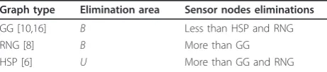
In general, all the mentioned graphs reduce the degree of the sensor nodes to shorten the routing delay on each node. As a consequence, many shortest paths in terms of the Euclidean distances are discarded between any pair of sensor nodes. Moreover, some least power paths between sensor nodes are unfortunately lost. Further-more, Shu et al. [11] mention that although GG and RNG are planar graphs, the delay for the multimedia WSNs based on these graphs is dramatically increased. As a summary, Table 1 demonstrates the differences between all the mentioned graphs in terms of different behaviors and definitions.

The reasons that GG eliminates few edges compared to RNG and HSP are as follows. First, GG has a bounded elimination area (i.e., circle) compared to the HSP (i.e., open half plane). Second, GG’s circular forbid-den area exists in the RNG’s elimination area (i.e., in the forbidden area constructed from the intersected of two circular areas).

3. An integration of clustering, routing, and topology control approaches

In this section, we introduce an integrated framework referred to as the CRTCA for WSNs. We incrementally integrate the proposed clustering, routing, and topology control approaches to construct the framework. We begin with the zone creation and active nodes selection that is followed by establishing paths among active nodes to the BS. Each of the integrated components is presented in the following sections.

3.1. Zone creation and active node selection

Once sensors are localized, the network area is divided into a number of zones. The BS assigns the sensor nodes to different zones based on their geometric positions.

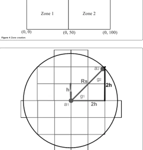
For instance, if the network area is very small (e.g., 100 m × 100 m) and divided into four zones, then sen-sor nodes are distributed as follows. Nodes with posi-tions between (0, 0) and (50, 50) reside in Zone 1. Whereas sensor nodes with positions between (50, 0) and (100, 50) reside in Zone 2. Figure 4 illustrates the zones construction where the BS is located outside of those zones.

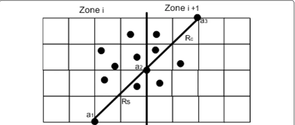
Afterwards, a minimum number of active sensor nodes are chosen by the BS and it works as follows. Each zone is divided into squares where each square has at least one active sensor node. However, even if this assumption does not hold, the region of that square is sensed by an active node of the neighboring squares. This is because an active sensor node in a square has the sensing coverage of all the neighboring squares (Fig-ure 5). Therefore, a very high probability of not having a sensing hole in the network is achieved. As a result, fault tolerance is accomplished. For instance, whenever the active sensor node of a square g1 fails, the network

operation (i.e., sending and receiving messages) pro-ceeds. This is done without activating another sensor node for that square or re-establishing the network topology. This is because the active node of the neigh-boring square ofg1 fully coversg1.

Using this topological structure, there is a high prob-ability that no sensing hole exists in the network if (see

Figure 5). The terms hand Rs is the side of a square

and the sensing range, respectively. Let us consider the following. The active sensor node a1of square g1 exists

at the bottom left corner and the active node a2 of

square g2 exists at the top right corner. If the nodea2

fails, then the squareg2 can still be covered by the node a1 of square g1. This is even if no other neighboring

square of g2 has active node. This is explained as

fol-lows. The farthest point p2 of g2 is within the sensing

range ofa1. By following Pythagoras formula, the square

coverage is possible. Figure 5 also clarifies this relation-ship betweenRsandh.

This topological structure also ensures that several active sensor nodes (i.e., at least one sensor node) of a zone reside within the communication range (Rc) of the

active nodes of the neighboring zones. This enables the sensor nodes to transmit the data to the BS through active nodes in their neighboring zones. This is because

Rc>Rsand there is a defined relationship between those

ranges [1]. In Figure 6, we find that sensor node a2 is at

the border of two zones Zi and Zi+1. Sensor nodes a1

anda2 are atRsapart. In addition, sensor nodes a1and a3 are atRcapart. In addition, a large number of nodes

in Zi+1 reside within the Rc of node a1 of Zone Zi.

Using this topological structure even if a small number of sensor nodes are distributed into the zones, the net-work is still expected to be covered. The reason is that each sensor node in a square covers all surrounding squares.

The BS chooses a CH for each zone. The chosen node is responsible for controlling the zone as well as select-ing active nodes of a zone. The criterion for choosselect-ing the CH is as follows. Based on our assumption that all sensor nodes initially have the same residual energy, the BS randomly chooses a sensor node. The chosen node Table 1 Differences between GG, RNG, and HSP graphs

Graph type Elimination area Sensor nodes eliminations

GG [10,16] B Less than HSP and RNG

RNG [8] B More than GG

HSP [6] U More than GG and RNG

(6)

Figure 4Zone creation.

Figure 5Zone-based topology where the sensing range. _R_s_{= 2}√₂_h.

(7)

becomes the CH. If the residual energy of the sensor nodes varies, the sensor node with the highest residual energy is chosen as CH. Then, the CH chooses active nodes in each zone based on (1) residual energy, (2) dis-tance, (3) number of sleep rounds, and (4) free buffer spaces. If only one sensor node is located in a square, then it is chosen as an active node. Otherwise, having

the same residual energy in nodes, say Aand Bin the

same zone, node Ais chosen as an active node. This is

when nodeAis closer to the BS than Bor active nodes

of neighboring zones. Further ties are broken by com-paring the remaining storage space or the number of sleep rounds of a node. Especially, node Ais given more priority if it has more remaining storage space compared

to node B. All other sensor nodes except the chosen

active nodes remain in sleep mode. This is done by turning their sensing and transmission radios off. Thus, a number of active nodes are determined in each zone. The determined number of sensor nodes provides a high probability that these nodes provide the sensing coverage of the whole network. Then, each active node generates the shortest path to the BS. Once the CH and active nodes are chosen, they work for a certain period of time (or rounds). They stop working once their resi-dual energy goes below a threshold value. After the clus-tering technique is proposed, we proceed with the second component of the proposed framework as follows.

3.2. Path establishment method

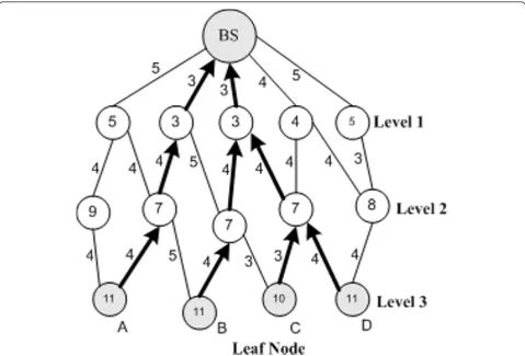
The path establishment method works as follows. Sensor nodes at levelL1 calculate their distances to the BS and

send this distance information to the sensor nodes at

levelL2. Then, nodes at level L2calculate their distances

to the sensor nodes at level L1 and then calculate the

total distance to the BS. This is done through different active nodes at levelL1. Thus, active nodes at the level L2find out the shortest path to the BS (see Figure 7).

Similarly, nodes at level Lkcompute the total distance

of the neighboring nodes at the upper levelLk-1to the

BS. Afterwards, these nodes identify the shortest path to the BS. Based on this information, an active node cre-ates a communication path with the neighboring active nodes. As a result, the total distance to the BS as well as the power consumptions is minimized as compared to existing tree-based routing protocols since power con-sumptions are proportional to the distance of transmis-sion path.

Moreover, each active sensor nodex at the level Li

chooses another active sensor nodey at the levelLi-1

with whichx has the second lowest distance to the BS.

The sensor nodey acts as an alternative node or as an

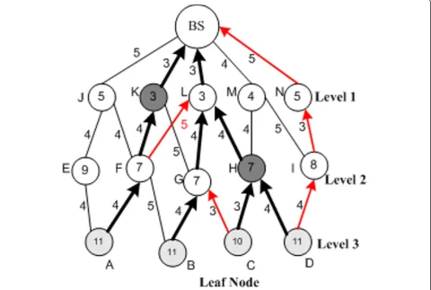
intermediate node of an alternative path for each leaf node to the BS. This enables the leaf node to transmit data to the BS in case of any active node fails. Once the paths are established, active nodes sense and route the data to the BS. Figure 7 demonstrates the path establish-ment method, where the shortest path from a leaf node to the BS is represented by bold arrows. Figure 8 illus-trates the alternative path establishment and the trans-mission of data through alternative node when an active sensor node fails. For instance, if node Kat level 1 fails,

active sensor node F at level 2 transmits data through

node L. The alternative path is shown as red arrows.

Based on the proposed framework, a new set of graphs for underlying topologies is proposed as follows.

(8)

3.3. A set of topology control algorithms

We introduce a new set of graphs referred to as the MG geometric graphs. These graphs are sub-graphs of the

UDGs. Each sensor node, u, running these graphs

chooses the nearest neighboring node, v. Afterwards, a

midpoint mid is calculated between the sensor nodes u

and v. As a result, a circlecis constructed with a center located at mid with a radiusr_midequal to s (|uv|/2).

The term sis a constant parameter within the range of

[0, 1] which shortens or increases ther_mid. If c con-tains a sensor node, sayw, in its area, then the edge [u,

v] is removed. Otherwise, the edge [u,v] is preserved. The algorithm proceeds on each sensor node until the network originally modeled by the UDG is recon-structed. This construction is based on a givens value. Because the MG only needs the position of the sensor node running this algorithm (i.e., current sensor node) as well as its neighboring nodes, this algorithm is there-fore local. Ifs is equal to1, then a special case of the graph is constructed, a GG [7,10]. However, the new set of graphs preserves more edges by using smaller circles and it may have crossing edges (i.e., non-planar graphs ifs ≠1). This is compared to that circle constructed by the GG. The possibility of maintaining shorter paths is

therefore increased in the MG. This is compared to the GG which makes the MG a denser graph. The MG runs in O(l*l) where lis the degree of sensor nodes. This is

because each time a sensor node, sayu, runs the MG,

chooses the nearest neighbor. Afterword, u checks all

the possible neighbors if they are inside the circle con-structed. In addition, the algorithm behaves locally which means that the complexity is analyzed per one

sensor node. For completeness, the MG’s algorithm is

included as shown in Algorithm 1 (appendix).

In the following section, we present the last frame-work’s component, i.e., the routing sensors data.

3.4. Routing of sensors data

The proposed routing protocol has two phases: (1) setup and (2) steady phase. The setup phase includes zones creation, active nodes selection, and path establishment.

All the framework’s components are based on MG and

GG. In the steady phase, data are transmitted from the source active node to the BS through intermediate active nodes. Active nodes at different levels work using TDMA scheme. The length of the timeslots at different levels is variable. For instance, at Timeslot 1, the active

nodes at the farthest level Lk sense the subscribed

Figure 7Shortest paths from leaf nodes to BS using path establishment method. Karimet al.EURASIP Journal on Wireless Communications and Networking2012,2012:120 http://jwcn.eurasipjournals.com/content/2012/1/120

(9)

events. Furthermore, the nodes send the corresponding data to active nodes at upper levelLk-1. At Timeslot 2,

active nodes at the levelLk-1receive data packet. These

nodes send acknowledgements to nodes at the levelLk.

Moreover, they transmit data packet to nodes at the

upper level Lk-2. Hence, the length of Timeslot 1 is

shorter than that of Timeslot 2.

The network is scalable since when more nodes are added to the network BS assigns zone ID to each node based on their locations and notifies CH without initiat-ing any network setup phase. These nodes will be con-sidered to be selected as active nodes whenever the setup phase is initiated after a certain number of rounds,

numOfRound, based on the current network energy sta-tus.

numOfRound= prevNoOfRounds

prevNetEnergy ×currentNetEnergy (1)

4. Performance evaluation

In this section, we present the energy model, the perfor-mance metrics, and the simulation model we have used

for performance evaluation. Furthermore, we show the simulation results for the proposed CRTCA and its var-iant with Gabriel (GG) and MG graphs.

4.1. Energy model

The energy consumption of a sensor node for sending a

data packet of size ndata bytes to another sensor node

(orCH) at the distancedis

ETX=ndata×εdata+ndata×d2×εair (2)

The energy consumptions of a node for receiving data

ERX=ndataεdata (3)

In Equation (2), εdata represents energy spent in

trans-mitter electronics circuitry (50 nJ/bit) and in Equation (3), εair represents energy consumptions in radio

ampli-fier for propagation loss (10 pJ/bit/m2). Receiving energy consumptions of a sensor does not have energy con-sumptions of radio amplifier for propagation loss.

4.2. Simulation model and performance metrics

(10)

programming language. We use randomly connected UDGs on an area of 100 m × 100 m as a basis of our simulation model. BS divides the network into a number zone and CH selects a number of active nodes in each zone that establish path to BS. The co-ordinate of the BS is assumed to be at 55 × 101.

The evaluation is done in terms of the following: (a) network energy consumptions (i.e., transmission and receiving power), (b) transmission energy consumptions, (c) end-to-end data transmission delay, (d) accumulated routing delays, and (e) length of the paths in terms of the crossed hops. Network energy consumption is defined as the total energy consumed by all the sensors nodes for routing data over a certain period of time. Network energy consumptions also reflect the lifetime of the net-work, i.e., the remaining network energy. We measure the end-to-end delay as the time that is required to trans-mit data from any source sensor node to the BS based on the traversed Euclidean distances. Another type of delay is in terms of the routing delay. Using this metric, the accumulated routing delays from any source sensor node to the BS are measured. Between these pairs of nodes, we also use another metric that counts the number of hops traversed on the path way which actually measures the network’s paths lengths.

Some simulation runs measure these metrics by either varying the followings: (1) the number of rounds (num_r) (i.e., from 10000 to 40,000 of an increment of 10,000) and (2) the number of zonesa(num_z) (i.e., from

4 to 10 of an increment of 2). When varyingnum_r, we

fixnum_zand the number of sensor nodes (num_sens) to 4 and 120, respectively. However, when we vary the

num_z, we fix the num_rand thenum_sens to 10,000 and 120, respectively. For all these simulation runs, the

constantsfor the MG graph is varied from 0.25 to 0.75

with an increment of 0.25.

Lastly, the connectivity of the network based on the MG is determined by measuring the Largest Connected Component. If this component was equal to the total number of sensor nodes in the network, then the net-work would have to be connected.

4.3. Simulation results

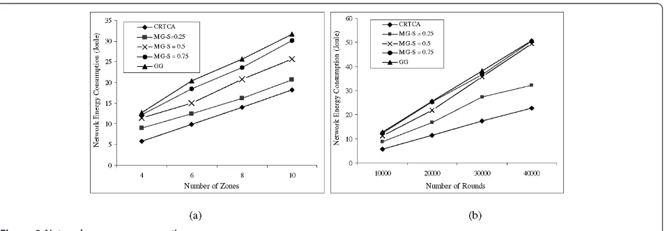
Figure 9a,b illustrates the total network energy con-sumptions varying the number of zones in the network and number of rounds, respectively. In both cases, the CRTCA outperforms other approaches. The same obser-vation applies even ifsis varied for the MG. This beha-vior is due to the high number of intermediate sensor nodes along the source-destination paths constructed by the CRTCA-GG and the CRTCA-MG. In other words, increasing the values ofs also increases the radius for the circular forbidden area where the intermediate nodes reside. Thus, more sensor nodes expose their bat-tery power. As a consequence, the total network energy consumptions for the CRTCA-GG and the CRTCA-MG are more than that for the CRTCA. It is also evident that if there are more intermediate nodes on a path in GG and MG, the receptions energy consumptions at the intermediate nodes will contribute to the larger network energy consumptions.

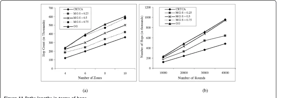
Hence, we evaluate their performance in terms of only the transmission energy consumptions which are illu-strated in Figure 10a,b. Again, we find that CRTCA out-performs the CRTCA-GG and CRTCA-MG. This is because more number of transmissions through the intermediate nodes will have more overhead energy consumptions of radio amplifier for propagation loss. Figure 11a,b supports the previous explanation by show-ing that the CRTCA maintains more number of shorter paths in terms of hops compared to those paths tra-versed by the other approaches.

Figure 9Network energy consumptions.

(11)

From all the previous simulation runs, an interesting

behavior for the set of MGs is demonstrated when sis

varied. The behavior is as follows: whens increases the possibility for loosing edges increases as the radius for the circular forbidden area increases. As a consequence, more intermediate nodes are selected for transmitting data from a source node to the destinations that results more network energy consumptions, transmission energy consumptions, and number of hops.

In Figure 12a,b, we find that the CRTCA-MG and CRTCA outperforms the CRTCA-GG in terms of the end-to-end delay. This is because the MG keeps more edges compared to those for the GG. As a result, shorter paths are discovered by the CRTCA-MG which significantly improves the transmission delay.

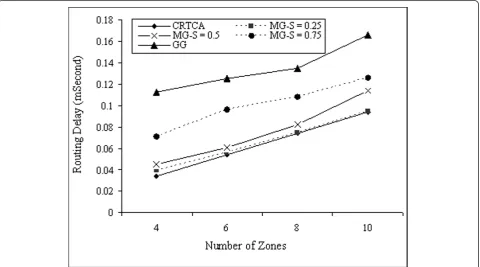
Finally, Figure 13 demonstrates the routing delay for varying the number of zones. Again, CRTCA outper-forms both MG and GG since in CRTCA, a path has less number of intermediate nodes and thus, delay for

making routing decision will be less as compared to MG and GG which have more intermediate nodes on a data path.

In general, the above results demonstrate that CRTCA outperforms MG and GG in most cases. For instance, as the number of zones increases the number of levels in the hierarchy also increases. As a consequence, the number of sensor nodes is decreased in each subzone of a level. Therefore, the average degree of sensor nodes is decreased. Furthermore, because of the nature for the MG and the GG, more edges are removed. Thus, longer paths are achieved between any pair of sensor nodes in the GG and the MG that contribute to more network energy consumptions, transmission energy consump-tions, and end-to-end delay. We also perform student’s

t-test at 95% confidence level which reveals the same

phenomenon, as are demonstrated and stated. However, all these simulations demonstrate that the MG achieves the connectivity property.

Figure 10Transmission energy consumptions.

(12)

5. Conclusion and future work

In this article, we introduced a framework for WSN that combines clustering, routing, and topology control approaches. We refer to the framework as CRTCA. This framework uses an efficient zone-based topology and routing protocol. Moreover, a new set of graphs are used as underlying topologies for the framework referred to as the MG graph. We find that the CRTCA based on the proposed new set of MG graphs (CRTCA-MG) outperforms the same framework based on an existing Gabriel graph (CRTCA-GG) in terms of the network energy consumptions, transmission energy

consumptions, end-to-end data transmission delay, rout-ing delay, and number of hops in the established path. In addition, the CRTCA demonstrates the best perfor-mance in most cases over CRTCA-MG and CRTCA-GG except the statistical analysis using student’st-test at 95% confidence level reveals that both CRCTA and

CRTCA-MG at lower value ofs have the same

perfor-mance in terms of end-to-end delay. Moreover, the MG demonstrates that it achieves the connectivity property. In the future, we will theoretically prove some geometric properties for the MG graphs. Furthermore, we will evaluate the framework by varying the number of nodes Figure 12End-to-end data transmission delay.

Figure 13Routing delay varying number of zones.

(13)

and the constants and in terms of additional defined metrics.

Appendix

Algorithm 1. MG(G,s)graph algorithm

Input: A graph G with the sensor node setVand a

parameters.

Output: A list of undirected edgesLfor each sensor

node u Î Vwhich represents the MG subgraph of G,

MG(G).

for allnodeuÎVdo

Create a list of neighbors ofu:LN(u) =N(u).L= ø. repeat

(a) Remove the nearest neighbor sensor nodevfrom

LN(u).

It also implies the number of levels in the virtual hier-archical structure of WSN.

A short version of this paper (6 pages) has appeared in the proceedings of IEEE WiMob 2011.

Author details 1

School of Computer Science, University of Guelph, Guelph, ON, Canada

2_{Electrical & Computer Engineering Department, College of Engineering,}

Alfaisal University, Saudi Arabia

Competing interests

The authors declare that they have no competing interests.

Received: 30 October 2011 Accepted: 27 March 2012 Published: 27 March 2012

References

1. F Chiti, A De Cristofaro, R Fantacci, D Tarchi, G Collodo, G Giorgett, A Manes, Energy efficient routing algorithms for application to agro-food wireless sensor networks, inProceedings of the IEEE International Conference on Communication (ICC), Seoul, Korea, pp. 3063–3067 (May 2005) 2. P Jacques, R Seshagiri, TV Prabhakar, H Jean-Pierre, HS Jamadagni,

COMMONSense Net: a wireless sensor network for resource-poor agriculture in the semiarid areas of developing countries. J Inf Technol Int. 4(1), 51_–67 (2007). doi:10.1162/itid.2007.4.1.51

3. S Yoo, J Kim, T Kim, S Ahn, J Sung, D Kim, A2_{S: automated agriculture}

system based on WSN, inPaper presented at the IEEE International Symposium on Consumer Electronics (ISCE), Dallas, TX, USA, pp. 1–5 (June 2007)

4. AH Kabashi, JMH Elmirghani, A technical framework for designing wireless sensor networks for agricultural monitoring in developing countries. in Paper presented at the International Conference on Next Generation Mobile Applications, Services and Technologies (NGMAST), Cardiff 395–401 (September 2008).

5. LK Kait, CZ Kai, R Khoshdelniat, SM Lim, EH Tat, Paddy growth monitoring with wireless sensor networks, inPaper presented at the International Conference on Intelligent and Advanced Systems (ICIAS), Kuala Lumpur, Malaysia, pp. 966_–970 (November 2007)

6. Z Haas, M Pearlman, The performance of query control schemes for the zone routing protocol. IEEE/ACM Trans Netw (TON).9(4), 427–438 (2001). doi:10.1109/90.944341

7. K Gabriel, R Sokal, A new statistical approach to geographic variation analysis. Syst Zool.18, 259–278 (1969). doi:10.2307/2412323

8. E Chavez, S Dobrev, E Kranakis, J Opatrny, L Stacho, H Tejeda, J Urrutia, Half-space proximal: a new local test for extracting a bounded dilation spanner, inProceedings of the International Conference On Principles of Distributed Systems, vol. 3974. Pisa, Italy, pp. 235–245 (2006)

9. G Toussaint, The relative neighborhood graph of finite planar set. Pattern Recogn.12(4), 261–268 (1980). doi:10.1016/0031-3203(80)90066-7 10. D Matula, R Sokal, Properties of gabriel graphs relevant to geographic

variation research and the clustering of points in the plane. Geograph Anal. 12(3), 205–222 (1980)

11. L Shu, Y Zhang, LT Yang, Y Wang, M Hauswirth, NX Xiong, TPGF: geographic routing in wireless multimedia sensor networks. Telecommun Syst.44(1-2), 79_–95 (2010). doi:10.1007/s11235-009-9227-0

12. S Liu, T Fevens, A Abdallah, Hybrid position-based routing algorithms for 3D mobile ad hoc networks, inPaper presented at the 4th International Conference on Mobile Ad-hoc and Sensor Networks, Wu Yi Mountain, China, pp. 177–186 (2008)

13. Z Yuan, L Wang, L Shu, T Hara, Z Qin, A balanced energy consumption sleep scheduling algorithm in wireless sensor networks, inWireless Communications and Mobile Computing Conference (IWCMC), Istanbul, Turkey, pp. 831–835 (July 2011)

14. R Chen, Z Zhong, M Ni, Cluster based iterative GPS-free localization for wireless sensor networks, inVehicular Technology Conference (VTC Spring), 2011 IEEE 73rd, Budapest, Hungary, pp. 1_–5 (May 2011)

15. G Xing, C Lu, R Pless, Q Huang, Impact of sensing coverage on greedy geographic routing algorithms. IEEE Trans Parallel Distrib Syst.17(4), 348–360 (2006)

16. W Yang, H Liusheng, W Junmin, X Hongli, Wireless sensor networks for intensive irrigated agriculture, inPaper presented at the Consumer Communications and Networking Conference (CCNC), Las Vegas, NV, USA, pp. 197_–201 (January 2011)

17. W Ke, W Liqiang, C Shiyu, Q Song, An energy-saving algorithm of WSN based on gabriel graph, in5th International Conference on Wireless Communications, Networking and Mobile Computing (WiCOM), Beijing, China, pp. 1_–4 (September 2009)

doi:10.1186/1687-1499-2012-120

Cite this article as:Karimet al.:The significant impact of a set of topologies on wireless sensor networks.EURASIP Journal on Wireless Communications and Networking20122012:120.

Submit your manuscript to a

journal and benefi t from:

7Convenient online submission 7Rigorous peer review

7Immediate publication on acceptance 7Open access: articles freely available online 7High visibility within the fi eld

7Retaining the copyright to your article