On solving some functional equations

(1)

R E S E A R C H

Open Access

On solving some functional equations

Dmitry V Kruchinin

*

*_{Correspondence:}

[email protected] Tomsk State University of Control Systems and Radioelectronics (TUSUR), Tomsk, Russia National Research Tomsk Polytechnic University (TPU), Tomsk, Russia

Abstract

Using the notion of composita and the Lagrange inversion theorem, we present techniques for solving the following functional equationB(x) =H(xB(x)m_{), where}_H₍_x_),

B(x) are generating functions andm∈N. Also we give some examples.

MSC: Primary 05A15; secondary 65Q20; 39B12

Keywords: composita; generating function; Lagrange inversion theorem; functional equation

1 Introduction

In this paper we study the coeﬃcients of the powers of an ordinary generating function and their properties. Using the notion of composita, we get the solution of the functional equationB(x) =H(xB(x)m_{), which is based on the Lagrange inversion equation, where}

H(x),B(x) are generating functions andm∈N.

In the papers [–], the author introduced the notion ofcompositaof a given ordinary generating functionF(x) =_n_>f(n)xn.

SupposeF(x) =_n_>f(n)xn_{is the generating function, in which there is no free term}

f() = . From this generating function we can write the following equation:

F(x)k=

n>

F(n,k)xn. ()

The expressionF(n,k) is thecomposita, and it is denoted byF₍_n_,_k_).

Deﬁnition  Thecompositais the function of two variables deﬁned by

F₍_n_,_k_{) =} πk∈Cn

f(λ)f(λ)· · ·f(λk), ()

whereCnis a set of all compositions of an integern,πkis the composition

k

i=λi=ninto

kparts exactly.

The expressionF₍_n_,_k_{) takes a triangular form}

F ,

F

, F,

F

, F, F,

F

, F, F, F,

..

. ... ... ... ...

F

n, Fn, . . . Fn,n– Fn,n

(2)

2 Lagrange inversion equation

First we consider a solution of the functional equation

A(x) =xHA(x), ()

whereA(x) andH(x) are generating functions such thatH(x) =_n≥_h(n)xnandA(x) =

n>a(n)xn.

In the following lemma, we give the Lagrange inversion formula, which was proved by Stanley [].

Lemma (The Lagrange inversion formula) Suppose H(x) =_n≥_h(n)xnwith h()= ,

and let A(x)be deﬁned by

A(x) =xHA(x). ()

Then

nxnA(x)k=kxn–kH(x)n, ()

where[xn_]_A₍_x₎k_{is the coeﬃcient of x}n_{in A}₍_x₎k_and_[_xn–k_]_H₍_x₎n_{is the coeﬃcient of x}n–k_in

H(x)n_.

By using the above Lemma , we now give the following theorem.

Theorem  Suppose H(x) =_n≥_h(n)xn_{is a generating function}_,_{where h}_()_{= ,}_H x(n,k)

is the composita of the generating function xH(x),and A(x) =_n_>a(n)xn_{is the}

generat-ing function,which is obtained from the functional equation A(x) =xH(A(x)).Then the following condition holds true:

A(n,k) =k

nH

x(n–k,n). ()

Proof According to Lemma , for the solution of the functional equationA(x) =xH(A(x)), we can write

nxnA(x)k=kxn–kH(x)n.

On the left-hand side, there is the composita of the generating functionA(x) multiplied byn:

nxnA(x)k=nA₍_n_,_k_).

We know that

xH(x)k=

n≥k

(3)

Then

H(x)k=

n≥k

H_x(n,k)xn–k.

If we replacen–kbym, we obtain the following expression:

H(x)k=

m≥

H

x(m+k,k)xm.

Substitutingnforkandn–kform, we get

xn–kH(x)n=H_x(n–k,n).

Therefore, we get

A(n,k) =k

nH

x(n–k,n).

According to the above theorem, for solutions of the functional equation A(x) =

xH(A(x)), we can use the following expression:

A(x)k=

n≥k

A(n,k)xn=

n≥k

k nH

x(n–k,n)xn,

whereH

x(n,k) is the composita of the generating functionxH(x). Therefore,

A(x) =

n≥



nH

x(n– ,n)xn. ()

Since the composita is uniquely determined by the generating function, formula () pro-vides a solution of the inverse equationA(x) =xH(A(x)), whenA(x) is known andH(x) is unknown. Hence,

H_x(n,k) = k k–nA

(k, k–n).

It should be noted that forn=k,

H_x(n,n) =A(n,n).

Next we give some examples of functional equations.

Example  Let us ﬁnd an expression for coeﬃcients of the generating functionA(x) =

n>a(n)xn, which is deﬁned by the functional equation

A(x) =x+xA(x) +xA(x)_{+ }_xA₍_x₎_.

The generating functionxH(x) has the form

(4)

The composita ofxH(x) is

According to formula (), the coeﬃcients ofA(x) are

a(n) = 

Example  Let us ﬁnd an expression for coeﬃcients of the generating function B(x) =

Next we introduce the following generating functionA(x) =xB(x). Considering the func-tional equation, we can notice that

A(x) =x +A(x) +A(x)



 –A(x) .

Then we get the following functional equation:

(5)

Hence, using Theorem , we get the composita ofA(x),

3 The generalized Lagrange inversion equation

Next we generalize the caseA(x) =xH(A(x)).

ReplacingA(x) byxB(x) in the functional equation (), we get

B(x) =HxB(x). ()

Let us introduce the following deﬁnitions.

Deﬁnition  The left composita of the generating functionB(x) in the functional equa-tion () is the composita

H

Deﬁnition  The right composita of the generating functionH(x) in the functional equa-tion () is the composita

B_x(n,k) =k

There exists the left composita for every left composita and there exists the right com-posita for every right comcom-posita.

Formula () can be generalized for the case when a generating function is the solution of a certain functional equation. Let us prove the following theorem.

Theorem  Suppose H(x) =_n≥_h(n)xn_{and B}₍_x_{) =}

n≥b(n)xnare generating functions

such that B(x) =H(xB(x)m_),_{where m}_∈_N_;_H

x(n,k)and Bx(n,k)are the compositae of the

generating functions xH(x)and xB(x),respectively.Then

B_x(n,k) = k

im–

H_x(im,im–), ()

(6)

Proof Form= , we have

B(x) =HxB(x)=G(x), im–=k,im=n.

Then we obtain the identity

B x(n,k) =

k kH

x(n,k).

Form= , we have

B(x) =G

xB(x)

, im–=n,im= n–k.

Then we obtain

B_x_,(n,k) = k

nH

x(n–k,n)

that satisfy Theorem .

By induction, we put that formthe solution of the equation

Bm(x) =H

xBm(x)m

()

is

B_x_,_m(n,k) = k

im–

H_x(im,im–).

Then we ﬁnd the solution form+ ,

Bm+(x) =H

xBm+(x)m+

.

For this purpose, we consider the following functional equation:

Bm+(x) =Bm

xBm+(x)

.

Instead ofBm(x), we substitute the right hand-side of ()

Bm+(x) =H

xBm+(x)

Bm

xBm+(x)

m

;

from whence it follows that

Bm+(x) =H

xBm+(x)m+

.

We note thatB

x,m+(n,k) is the right composita ofBm(x),

B_x_,_m_+(n,k) =k

nB

x,m(n–k,n),

whereB

(7)

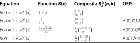
Table 1 Table of functional equations

Equation FunctionB(x) CompositaBx(n, k) OEIS

B(x) = 1 +xB0_(x) _{1 +}_x k n–k

B(x) = 1 +xB1_(x) 1 1–x

n–1 k–1

A000012

B(x) = 1 +xB2_(x) 1–√1–4x 2x

k n

2n–k–1 n–1

A000108

B(x) = 1 +xB3_(x) k n

3n–2k n–k

A001764

Then

B_x_,_m_+(n,k) = k

(m+ )n–mkH

x

(m+ )n– (m+ )k, (m+ )n–mk.

Therefore, for the functional equation

Bm+(x) =Bm

xBm+(x)

,

we obtain the required condition

B_x_,_m_+(n,k) = k

im

H_x(im+,im),

whereim= (m+ )n–mk.

In Table  we present a sequence of functional equations for the generating function

H(x) =  +x, where OEIS means the On-Line Encyclopedia of Integer Sequences [].

Competing interests

The author declares that they have no competing interests.

Acknowledgements

The author wishes to thank the referees for their useful comments. This work was partially supported by the Ministry of Education and Science of Russia, government order No. 1220 ‘Theoretical bases of designing informational-safe systems’.

Received: 30 October 2014 Accepted: 25 December 2014

References

1. Kruchinin, VV, Kruchinin, DV: Composita and its properties. J. Anal. Number Theory2(2), 1-8 (2014) 2. Kruchinin, DV, Kruchinin, VV: A method for obtaining generating function for central coeﬃcients of triangles.

J. Integer Seq.15, 1-10 (2012)

3. Kruchinin, DV, Kruchinin, VV: Application of a composition of generating functions for obtaining explicit formulas of polynomials. J. Math. Anal. Appl.404, 161-171 (2013)

4. Stanley, RP: Enumerative Combinatorics, vol. 2. Cambridge Studies in Advanced Mathematics. Cambridge University Press, Cambridge (1999)