Resonant Elastic Scattering
Francois de Oliveira Santos
1GANIL,CEA/DSM-CNRS/IN2P3,BoulevardHenriBecquerel,CaenCedex5,F-14076,France e-mail: [email protected]
Abstract.Elastic scattering of nuclei at energies typically below 10 MeV/nucleon can be
used as a powerful method for studying nuclear spectroscopy. Resonances are observed in the excitation function, corresponding to unbound states in the compound nucleus. The analysis of the shape of these resonances can provide the excitation energy, the total width, the partial width, and the spin of the excited states.
1 The Rutherford scattering
The experimental study of nuclear collisions started when Marsden, Geiger, Rutherford and their collaborators directed alpha particles emitted by a radioactive source of radium onto different metallic foils (publication in 1909 [1]). They observed that a part of the alpha projectiles interacted "strongly" with the matter and back-scattered at large angles (beyond 90 degrees). In 1911, Rutherford published [2] an interpretation of these data. In his model, the atoms are made of a nucleus positively charged and containing most of the atomic mass, surrounding by a halo of light electrons negatively charged. The positively charged alpha particles were back-scattered by the strong Coulomb repulsion of the positively charged atomic nuclei. In 1914, Darwin [3] derived a formula for the cross section of this "Rutherford elastic scattering":
dσ
dΩRuther f ord=( Z1Z2e2 Esin(θ
2)
)2 (1)
whereZ2is the charge of the target nucleus,E andZ1 are the energy of the incident particle and its charge, scattered at center of mass angleθ(see Fig. 1 top left).
2 First observations of anomalies in the elastic scattering
The radioactive sources provide alpha particles with well defined energies. Different foils can be used to decelerate the particles to different lower energies. Then, it is possible to measure the excitation function, that is to say, the differential cross section as the function of the energy, and to compare it with the Rutherford scattering. According to the formula, the differential cross section should vary inversely proportional to the square of the energy. Deviations from this law were observed (Rutherford 1919 [5], Chadwick 1921 [6] ). Figure 2 shows the results obtained by Chadwick for the scattering of alpha particles onto an hydrogen target, compared to the expected results using the Rutherford scattering formula. Large deviations are observed at higher energies.
EPJ Web of Conferences 184, 01006 (2018) https://doi.org/10.1051/epjconf/201818401006
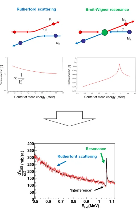
Figure 1.Top left: The Rutherford elastic scattering. The two nuclei undergo the strong Coulomb repulsion but they don’t "touch" each other. The cross section can be calculated with Eq. 1. Top right: The resonant elastic scattering. The two nuclei merge and make a compound nucleus which then decays to the elastic scattering channel. The cross section can be calculated with the Breit-Wigner formula. Bottom: Excitation function of the reaction14N(p,p)14N measured at GANIL [4] at the angle of 180◦CM. The data follow very well the Rutherford elastic scattering formula, except at the energy close to Elab ≃1.06 MeV where a resonance can be observed. It is interpreted as a resonance in the compound nucleus15O. As shown at energies below the maximum of the
resonance, the Rutherford and the resonant contributions interfere negatively.
3 Resonances in the elastic scattering
More precise measurements made later on different targets have revealed many deviations, generally localized at certain specific incident energies. For example, Fig. 1 (bottom) shows the excitation function of the elastic scattering reaction14N(p,p)14N measured at GANIL [4] at the angle of 180◦ CM. It is observed that the cross section follows very well the Rutherford elastic scattering formula, except for the energy close to Elab ≃1.06 MeV where a resonance can be observed. As it is shown
EPJ Web of Conferences 184, 01006 (2018) https://doi.org/10.1051/epjconf/201818401006
Figure 1.Top left: The Rutherford elastic scattering. The two nuclei undergo the strong Coulomb repulsion but they don’t "touch" each other. The cross section can be calculated with Eq. 1. Top right: The resonant elastic scattering. The two nuclei merge and make a compound nucleus which then decays to the elastic scattering channel. The cross section can be calculated with the Breit-Wigner formula. Bottom: Excitation function of the reaction14N(p,p)14N measured at GANIL [4] at the angle of 180◦CM. The data follow very well the Rutherford elastic scattering formula, except at the energy close to Elab ≃1.06 MeV where a resonance can be observed. It is interpreted as a resonance in the compound nucleus15O. As shown at energies below the maximum of the
resonance, the Rutherford and the resonant contributions interfere negatively.
3 Resonances in the elastic scattering
More precise measurements made later on different targets have revealed many deviations, generally localized at certain specific incident energies. For example, Fig. 1 (bottom) shows the excitation function of the elastic scattering reaction14N(p,p)14N measured at GANIL [4] at the angle of 180◦ CM. It is observed that the cross section follows very well the Rutherford elastic scattering formula, except for the energy close to Elab ≃1.06 MeV where a resonance can be observed. As it is shown
Figure 2.Square root of the differential cross section as a function of the square of the inverse of the projectile
velocity, measured for the reaction H(α,α)H. In these axis, the Rutherford scattering formula is a straight line (green). Deviations from the Rutherford formula are observed at higher energies.
in Fig.3, this resonance matches perfectly to the energy of an excited state in the compound nucleus 15O.
Figure 3.The energy Elab≃1.06 MeV of the resonance observed in Fig. 1, or ECM ≃0.985 MeV in center of mass, above the reaction threshold14N+p(S=7.2971 MeV), matches perfectly to the energy E
x=8.284 MeV of the 3/2+excited state in the compound nucleus15O: E
x=S+ECM. The resonance is due to the existence of this excited state.
Two different reaction mechanisms can be invoked to explain the measured data. On the one hand (Fig.1, top left), the two nuclei undergo the strong Coulomb repulsion but they don’t "touch" each other. On the other hand (Fig.1, top right), the two nuclei make a compound nucleus which decays to the elastic scattering channel. This reaction mechanism is called Resonant Elastic Scattering.
EPJ Web of Conferences 184, 01006 (2018) https://doi.org/10.1051/epjconf/201818401006
4 R-Matrix formalism
In reality, the two contributions, the Rutherford scattering and the resonant scattering, operate si-multaneously and are indistinguishable. The final cross section is not just the sum of the two cross sections, quantum mechanics says. Amplitude of probabilities should be added, resulting sometimes into interferences between the two contributions, see Fig.1 (bottom). The R-Matrix formalism can be used to calculate, to predict or to fit the excitation function of the elastic scattering including different contributions and their interferences. The theoretical developments of this formalism would take up too much space in this article, theoretical details can be obtained in other articles, see for example Ref[7, 8]. Here, the heuristic example (without Coulomb!): the case of the s-wave scattering of a spinless neutron by a square-well potential, will be presented.
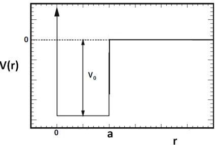
For simplicity, let’s assumed the potential between the target nucleus and the projectile to be a square well with a potential depth V0and a radiusr=a, see Fig. 4. The potential goes to infinity at r=0, and it is zero out tor=∞.
Figure 4.The potential between the target nucleus and the projectile is assumed be a square well with a potential depth V0and a radiusr=a.
In this simple case, two contributions are also expected: the elastic scattering from the square-well and the resonant scattering from the compound nucleus (the neutron in the mean field of the square well). The radial part of the Schrödinger equation
−2m2 d2drϕ(2r) + V0ϕ(r) = Eϕ(r) (2)
should be solved.
In the internal region (r<a), the solution is
ϕ(r)=Asin(K r) (3)
whereAis a constant andK= √2m(E+V0)/.
In the external region (r>a), it is possible to show that
ϕ(r)=B[e−ikr−e2iδe+ikr] (4)
EPJ Web of Conferences 184, 01006 (2018) https://doi.org/10.1051/epjconf/201818401006
4 R-Matrix formalism
In reality, the two contributions, the Rutherford scattering and the resonant scattering, operate si-multaneously and are indistinguishable. The final cross section is not just the sum of the two cross sections, quantum mechanics says. Amplitude of probabilities should be added, resulting sometimes into interferences between the two contributions, see Fig.1 (bottom). The R-Matrix formalism can be used to calculate, to predict or to fit the excitation function of the elastic scattering including different contributions and their interferences. The theoretical developments of this formalism would take up too much space in this article, theoretical details can be obtained in other articles, see for example Ref[7, 8]. Here, the heuristic example (without Coulomb!): the case of the s-wave scattering of a spinless neutron by a square-well potential, will be presented.
For simplicity, let’s assumed the potential between the target nucleus and the projectile to be a square well with a potential depth V0and a radiusr=a, see Fig. 4. The potential goes to infinity at r=0, and it is zero out tor=∞.
Figure 4.The potential between the target nucleus and the projectile is assumed be a square well with a potential depth V0and a radiusr=a.
In this simple case, two contributions are also expected: the elastic scattering from the square-well and the resonant scattering from the compound nucleus (the neutron in the mean field of the square well). The radial part of the Schrödinger equation
−2m2 d2drϕ(2r) + V0ϕ(r) = Eϕ(r) (2)
should be solved.
In the internal region (r<a), the solution is
ϕ(r)=Asin(K r) (3)
whereAis a constant andK= √2m(E+V0)/.
In the external region (r>a), it is possible to show that
ϕ(r)=B[e−ikr−e2iδe+ikr] (4)
and the cross section of the elastic scattering
σ(E)=4 π
k2sin2(δ) (5)
whereBis a constant,δis called the phase shift, it is a function of the energy, andk= √2m(|E|)/. The functionϕ(r) and its derivative should be continuous atr=a, this gives
δ=arctan[k
Ktan(Ka)]−ka (6)
This can be rewritten
δ=arctan[kϕ(a)
ϕ(a)′]−ka (7)
The internal wave function can always be expanded with a complete set of basics states Xλ(r)
ϕ(r)=∑
λ
CλXλ(r) (8)
whereCλare different coefficients. These coefficients can be obtained with the relation
Cλ=
∫ a
0 X
∗
λ(r)ϕ(r)dr (9)
The "resonant states" inside the square well are a good set of basics states. These "resonant states" can be obtained by solving the Schrödinger equation with the condition
dXλ
dr (r=a)=0 (10)
One obtains
Xλ(r)=(
2 a)1
/2sin(K
λr) (11)
with
Kλ=(λ+1
2)
π
a (12)
At r=a, one gets
Xλ(r=a)=(2
a)1
/2 (13)
Using the Schrödinger equations forϕ(r) and for Xλ(r), one can get
−2m2 {ddr2ϕ2X∗
λ−ϕ
d2X∗
λ
dr2 }=(E−Eλ)ϕX∗λ (14)
which gives after integration
−2m2 [ dϕ drX∗λ−ϕ
dX∗
λ
dr ]a0 = (E−Eλ)
∫ a
0 ϕX
∗
λdr (15)
which can be used in eq. 9, giving
Cλ= 2/2m Eλ−EX
∗
λ(a)ϕ ′
(a) (16)
EPJ Web of Conferences 184, 01006 (2018) https://doi.org/10.1051/epjconf/201818401006
Using this expression in eq.8, one gets
aϕ′(a)
ϕ(a) =
1 ∑
λ 2/ma2
Eλ−E
= 1
R (17)
where R is the R-function, i.e. R=∑λ γ 2
Eλ−E withγ
2 =2/ma2the reduced width. Eq. 17 can be used
in eq. 7, in the approximation of a single term inλ, i.e. R=Eγ2
λ−E, giving
4 sin2(δ) = |2 sin(ka)eika− Γ (Eλ−E)−iΓ2|
2 (18)
withΓ = 2kaγ2the level width, and for the cross section (eq.5)
σ(E)= π k2
�� �� ��
�2 sin(ka)e
ika− Γ (Eλ−E)−iΓ2
�� �� �� � 2
(19)
There are two terms in this expression. The first term corresponds to the elastic scattering onto a hard sphere (for which the potential is infinite forr < aand zero forr >a). If the second term is
neglected, when k goes to zero,σ(E)→4πa2, which is just the geometric cross section of the square
well. The second term corresponds to the Breit-Wigner resonance. The two terms may interfere since the two amplitudes are added before putting the sum to the square.
5 R-Matrix codes
There are two variants of the R-matrix formalism differing mainly by their types of applications [7]. In the calculable R-matrix, the aim is to accurately solve the Schrödinger equation mostly in the con-tinuum and predict reaction cross sections (predict resonances properties). In the phenomenological R-matrix, the goal is to parameterize scattering data (fit of data, predict cross sections from a given set of resonance properties).
Several codes exist "in the market" to calculate the scattering cross section according to the for-malism of the phenomenological R-matrix, and these are often available freely. The code "AZURE" is one of the latest and best users friendly codes. Without going into details, this code is very intu-itive. The particle pairs are described in a first tab (spin, separation energy etc.). The excited states of the compound nucleus are introduced as input parameters in a second tab (excitation energies, spins, widths etc.). That’s about it! More details can be obtained in the reference [9].
6 Pros and cons
Elastic scattering reactions can be used to study the structure of the compound nucleus:
• The energies Exof the excited states can be determine from the measured energies ERof the reso-nances, since Ex=ER+S, withS the particle-emission threshold, see Fig. 3.
• The scattering reaction is induced most often on protons, but other particles can also be used, like alpha particles.
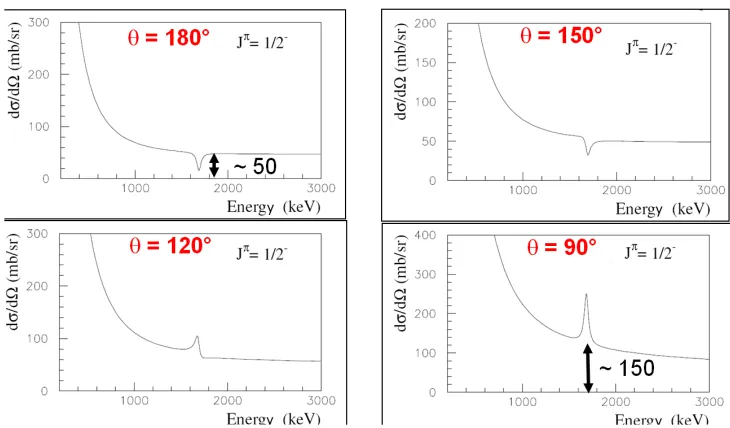
• Due to the interferences effects, the shape of the resonances depends on the spin of the states, see Fig. 5. Then, the analysis of the shape of the resonances can be used to assign or constrain the spins of the excited states.
EPJ Web of Conferences 184, 01006 (2018) https://doi.org/10.1051/epjconf/201818401006
Using this expression in eq.8, one gets
aϕ′(a)
ϕ(a) =
1 ∑
λ 2/ma2
Eλ−E
= 1
R (17)
where R is the R-function, i.e. R=∑λ γ 2
Eλ−E withγ
2=2/ma2the reduced width. Eq. 17 can be used
in eq. 7, in the approximation of a single term inλ, i.e. R=Eγ2
λ−E, giving
4 sin2(δ) = |2 sin(ka)eika− Γ (Eλ−E)−iΓ2|
2 (18)
withΓ = 2kaγ2the level width, and for the cross section (eq.5)
σ(E)= π k2
�� �� ��
�2 sin(ka)e
ika− Γ (Eλ−E)−iΓ2
�� �� �� � 2 (19)
There are two terms in this expression. The first term corresponds to the elastic scattering onto a hard sphere (for which the potential is infinite forr < aand zero forr > a). If the second term is
neglected, when k goes to zero,σ(E)→4πa2, which is just the geometric cross section of the square
well. The second term corresponds to the Breit-Wigner resonance. The two terms may interfere since the two amplitudes are added before putting the sum to the square.
5 R-Matrix codes
There are two variants of the R-matrix formalism differing mainly by their types of applications [7]. In the calculable R-matrix, the aim is to accurately solve the Schrödinger equation mostly in the con-tinuum and predict reaction cross sections (predict resonances properties). In the phenomenological R-matrix, the goal is to parameterize scattering data (fit of data, predict cross sections from a given set of resonance properties).
Several codes exist "in the market" to calculate the scattering cross section according to the for-malism of the phenomenological R-matrix, and these are often available freely. The code "AZURE" is one of the latest and best users friendly codes. Without going into details, this code is very intu-itive. The particle pairs are described in a first tab (spin, separation energy etc.). The excited states of the compound nucleus are introduced as input parameters in a second tab (excitation energies, spins, widths etc.). That’s about it! More details can be obtained in the reference [9].
6 Pros and cons
Elastic scattering reactions can be used to study the structure of the compound nucleus:
• The energies Exof the excited states can be determine from the measured energies ER of the reso-nances, since Ex=ER+S, withS the particle-emission threshold, see Fig. 3.
• The scattering reaction is induced most often on protons, but other particles can also be used, like alpha particles.
• Due to the interferences effects, the shape of the resonances depends on the spin of the states, see Fig. 5. Then, the analysis of the shape of the resonances can be used to assign or constrain the spins of the excited states.
Figure 5.Elastic scattering excitation functions calculated using the same experimental conditions and exactly the same properties of the state in the compound nucleus but with different spins. The analysis of the shape of
the resonance can be used to determine the spin of the states.
Figure 6. Elastic scattering excitation functions calculated for different angles in center of mass calculated for
the reaction12C+proton (from Ref. [10]). These spectra are calculated using exactly the same properties of the
resonant state in the compound nucleus. The analysis of the shape of the resonance as a function of the angle can be used to determine the spin of the state.
• The evolution of the excitation function with the angle of the scattered particles can also be used to determine the spin of the states, see Fig. 6, this is particularly useful when there are several resonances superposed.
• The width and the height of the resonances peaks can be used to measure the total and partial widths of the states.
• The differential cross sections are relatively high, typically several tens or hundreds of millibarns per steradian. Radioactive beams with relatively low intensities can be used.
EPJ Web of Conferences 184, 01006 (2018) https://doi.org/10.1051/epjconf/201818401006
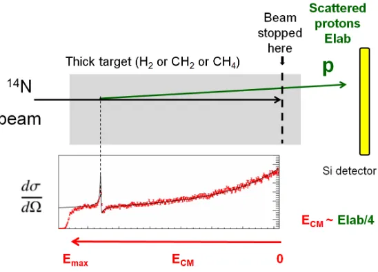
• It is possible to use a radioactive beam and to measure the elastic scattering in inverse kinematics (heavy ion onto a light target nucleus). The thick target inverse kinematics (TTIK) technique (thick enough to stop the beam inside the target), first proposed by V.Z. Goldberg [11], is very well adapted to these relatively low beams intensities. The center mass energy of the interaction point (reaction vertex) can be determined from the measured energy of the protons in the lab, after correction of the energy lost in the target. The center of mass angle is related to the lab angle byθCM = 2θlab (this relationship is quasi-true within the special relativity). The measured cross-section has to be corrected for different effects, mainly the fact that the effective target thickness is not constant. The energy of the scattered particles in lab is related to the center of mass energy by
Elab(scattered particle) = 4 mp
mp+mt ECMcos(θlab) (20) withmp andmt the projectile mass and the target mass. In the case θlab=0 and a proton target, ECM ≈ 14 Elab(proton). It is possible to obtain high energy resolution spectra even with a thick target (the center of mass energy resolution is about 4 times smaller than the energy resolution in the lab), see Fig. 7.
Figure 7.In the thick target technique in the case of the protons, if the energy loss of the scattered protons in the target is neglected,ECM ≈ 14 Elab(proton). The center of mass energy of the reaction vertex is determined from the measured energy of the protons in the lab, after correction of the small energy losses in the target.
• The energy resolution of the measured scattered protons can be estimated using the relation:
σLab = √
σ2det+σ2θ+σ2strag, where σdet is the energy resolution of the detector (σdet=9 keV in the14N setting of Fig. 1),σ
stragis the energy straggling in the target (estimated from simulations
to be lower than 5 keV in14N), andσ
θis the energy resolution due to the aperturedθof the
de-tector. In inverse kinematics, it can be derived thatσθ =tan(θ)Edθ. Therefore the degradation in
energy resolution is minimal whenθ=0◦. For this reason, and for maximizing the ratio between
EPJ Web of Conferences 184, 01006 (2018) https://doi.org/10.1051/epjconf/201818401006
• It is possible to use a radioactive beam and to measure the elastic scattering in inverse kinematics (heavy ion onto a light target nucleus). The thick target inverse kinematics (TTIK) technique (thick enough to stop the beam inside the target), first proposed by V.Z. Goldberg [11], is very well adapted to these relatively low beams intensities. The center mass energy of the interaction point (reaction vertex) can be determined from the measured energy of the protons in the lab, after correction of the energy lost in the target. The center of mass angle is related to the lab angle byθCM = 2θlab (this relationship is quasi-true within the special relativity). The measured cross-section has to be corrected for different effects, mainly the fact that the effective target thickness is not constant. The energy of the scattered particles in lab is related to the center of mass energy by
Elab(scattered particle) = 4 mp
mp+mt ECMcos(θlab) (20) withmp andmt the projectile mass and the target mass. In the caseθlab=0 and a proton target, ECM ≈ 14 Elab(proton). It is possible to obtain high energy resolution spectra even with a thick target (the center of mass energy resolution is about 4 times smaller than the energy resolution in the lab), see Fig. 7.
Figure 7.In the thick target technique in the case of the protons, if the energy loss of the scattered protons in the target is neglected,ECM ≈ 14 Elab(proton). The center of mass energy of the reaction vertex is determined from the measured energy of the protons in the lab, after correction of the small energy losses in the target.
• The energy resolution of the measured scattered protons can be estimated using the relation:
σLab = √
σ2det+σ2θ+σstra2 g, where σdet is the energy resolution of the detector (σdet=9 keV in the14N setting of Fig. 1),σ
stragis the energy straggling in the target (estimated from simulations
to be lower than 5 keV in14N), andσ
θis the energy resolution due to the aperturedθof the
de-tector. In inverse kinematics, it can be derived thatσθ =tan(θ)Edθ. Therefore the degradation in
energy resolution is minimal whenθ=0◦. For this reason, and for maximizing the ratio between
the nuclear and the Coulomb contribution in the differential cross-section (see Fig. 6), the scattered protons are generally measured at very forward angles. An energy resolution ofσLab ≈ 10 keV was measured in the case of14N, which lead toσCM ≃3 keV in the center of mass.
The resonant elastic scattering technique has some specific limitations: • Only states above the particle emission threshold can be studied.
• The number of counts measured in the peak is proportional to the width of the resonance. The narrower it is, the more beam time is needed to observe the peak.
• When the density of states is high, it is not possible to observe isolated resonances.
• It is not possible to observe the shape of the resonance nor the spin of the state when the resonance is narrower than the experimental energy resolution. But, if a thin target is used, it is possible to determine the cross section point by point using a beam accelerated to different energies. In principle, the energy resolution could be excellent (26 eV! in ref. [12]) provided the beam has a good energy resolution.
7 An informative experiment example
Several cases of resonant elastic scattering experiments were presented during the 2017 Santa Tecla School [13–20]. A very informative example is given in the article of Bardayanet al[21]. Knowledge of the astrophysical rate of the18F(p,α)15O reaction is important for understanding theγ-ray emis-sion expected from novae. The rate of this reaction is dominated at temperatures above 0.4 GK by a resonance near 7.08 MeV excitation energy in19Ne. In this study, the authors proposed to made simul-taneous measurements of the1H(18F,p)18F and1H(18F,α)15O excitation functions using a radioactive 18F beam at the ORNL Holifield Radioactive Ion Beam Facility. They used relatively thin target and radioactive beams accelerated to different energies. The R-Matrix analysis of the1H(18F,p)18F exci-tation function, see Fig. 8, provided many pieces of information needed to calculate the rate of the reaction. The cross section of the reaction1H(18F,α)15O, combined with these pieces of information, allowed to determine the spin of the state.
Acknowledgement
This publication was supported by OP RDE, MEYS Czech Republic under the project EF16-013/0001679,byLEANuAG,byLIACOSMAandbyLIACOLL-AGAIN.
References
[1] H. Geiger, E. Marsden, Proceedings of the Royal Society of London Series A82, 495 (1909) [2] E. Rutherford, Phil. Mag.6, 21 (1911)
[3] C. Darwin, Phil. Mag.XXVII, 499 (1914)
[4] I. Stefan, Ph.D. thesis (Université de Caen, France, 2006) [5] Rutherford, Phil. Mag.XXXVII, 537 (1919)
[6] J. Chadwick, Phil.Mag.42, N252, 923 (1921)
[7] P. Descouvemont, D. Baye, Reports on progress in physics73, 036301 (2010) [8] C.A. Bertulani,Nuclei in the Cosmos(World Scientific, 2014)
[9] R. Azuma, E. Uberseder, E. Simpson, C. Brune, H. Costantini, R. De Boer, J. Görres, M. Heil, P. LeBlanc, C. Ugalde et al., Physical Review C81, 045805 (2010)
EPJ Web of Conferences 184, 01006 (2018) https://doi.org/10.1051/epjconf/201818401006
Figure 8. The reactions1H(18F,p)18F and1H(18F,α)15O were measured in the same experiment simultaneously
[21]. The R-matrix formalism was used to fit the two spectra. Important spectroscopic information were ex-tracted.
[10] Lynda Achouri (Ph. D Thesis. Universite de Caen, 2001)
[11] V. Gol’Dberg, A. Pakhomov, Physics of Atomic Nuclei56, 1167 (1993)
[12] S. Wüstenbecker, H. Becker, H. Ebbing, W. Schulte, M. Berheide, M. Buschmann, C. Rolfs, G. Mitchell, J. Schweitzer, Zeitschrift für Physik A Hadrons and nuclei344, 205 (1992) [13] D. Torresi, L. Cosentino, P. Descouveont, A. Di Pietro, C. Ducoin, P. Figuera, M. Fisichella,
M. Lattuada, C. Maiolino, A. Musumarra et al.,8Li+αresonant elastic scattering: a tool to study cluster states in 12B, inJournal of Physics: Conference Series(IOP Publishing, 2014), Vol. 569, p. 012024
[14] H. Yamaguchi, D. Kahl, Y. Wakabayashi, S. Kubono, T. Hashimoto, S. Hayakawa, T. Kawabata, N. Iwasa, T. Teranishi, Y. Kwon et al., Physical Review C87, 034303 (2013)
[15] F. de Oliveira Santos, P. Himpe, M. Lewitowicz, I. Stefan, N. Smirnova, N. Achouri, J. Angélique, C. Angulo, L. Axelsson, D. Baiborodin et al., The European Physical Journal A-Hadrons and Nuclei24, 237 (2005)
[16] M. Freer, E. Casarejos, L. Achouri, C. Angulo, N. Ashwood, N. Curtis, P. Demaret, C. Harlin, B. Laurent, M. Milin et al., Physical review letters96, 042501 (2006)
[17] L. Axelsson, M.J.G. Borge, S. Fayans, V.Z. Goldberg, S. Grévy, D. Guillemaud-Mueller, B. Jon-son, K.M. Källman, T. Lönnroth, M. Lewitowicz et al., Phys. Rev. C54, R1511 (1996)
[18] M. Assie, F. de Oliveira Santos, T. Davinson, F. De Grancey, L. Achouri, J. Alcántara-Núñez, T. Al Kalanee, J.C. Angélique, C. Borcea, R. Borcea et al., Physics Letters B712, 198 (2012) [19] I. Stefan, F. de Oliveira Santos, O. Sorlin, T. Davinson, M. Lewitowicz, G. Dumitru,
J. Angélique, M. Angélique, E. Berthoumieux, C. Borcea et al., Physical Review C90, 014307 (2014)
[20] F. De Grancey, A. Mercenne, F. de Oliveira Santos, T. Davinson, O. Sorlin, J. Angélique, M. As-sié, E. Berthoumieux, R. Borcea, A. Buta et al., Physics Letters B758, 26 (2016)
[21] D. Bardayanet al., Phys. Rev. C63, 065802 (2001)
EPJ Web of Conferences 184, 01006 (2018) https://doi.org/10.1051/epjconf/201818401006


![Figure 8. The reactions 1H(18F,p)18F and 1H(18F,α)15O were measured in the same experiment simultaneously[21]](https://thumb-us.123doks.com/thumbv2/123dok_us/8037564.1337912/10.482.100.380.83.265/figure-reactions-h-f-f-measured-experiment-simultaneously.webp)
