ZHAO, MING. Design, Modeling, and Analysis of User Mobility and Its Impact on Multi-hop Wireless Networks. (Under the direction of Dr. Wenye Wang).
Due to the readily deployable and self-organizing nature of mobile ad hoc networks (MANETs), various demanding military and civilian applications are expected to be widely imple-mented in MANETs. The fundamental issue in MAENTs is that performance degrades dramatically as the increase of path failures due to the complexity of user mobility. Therefore, understanding the impacts and implications of user mobility is essential to the system design, topology control, and routing optimization in MANETs.
by Ming Zhao
A dissertation submitted to the Graduate Faculty of North Carolina State University
in partial fullfillment of the requirements for the Degree of
Doctor of Philosophy
Computer Engineering
Raleigh, North Carolina 2009
APPROVED BY:
Dr. Michael Devetsikiotis Dr. Khaled Harfoush
Dr. Wenye Wang Dr. Arne A. Nilsson
DEDICATION
To my parents
Bailing Zhao and Guirong Wang. To my wife and our son
Lu Qu and Alexander Tianhao Zhao. To my parents-in-law
BIOGRAPHY
ACKNOWLEDGMENTS
My deepest gratitude goes first and foremost to my advisor Dr. Wenye Wang. I cannot be thankful enough to Dr.Wang for her wisdom, knowledge, support, numerous inspirations and guidance. Without her endless effort and countless suport, my PH.D. dream would never become true. Without her guidance and persistent help, this dissertation would not have been possible to be completed. I have benefited immensely from her guidance in academic growth, career development and social behaviors in my life.
I would like to express the cordial appreciation to Dr. Arne A Nilsson, Dr. Michael Devetsikiotis, and Dr. Khaled Harfoush for serving on my committee and providing their invaluable comments and critical suggestions to help me achieve a successful doctoral study.
It was my pleasure and honor to have worked closely with my colleagues during my PH.D. study: Dr. Fei Xing, Dr. Nurcan Tezcan, Yi Xu, Avesh K. Algawal, Shawqi Kharbash, Dr. Xinbing Wang, Dr. Wei Liang, Jung Kee Song, Lei Sun, Entong Shen, Lifang Guo, Chi Yi, and Levi Mason. I have benefited significantly from enlightening discussions, research project study, and more important, life issue and spiritual support with them. They encouraged me often times when I faced the challenging research issues. I would like to thank them for all their help, support, and valuable hints. I wish to thank every my friend for all their help and caring they provided during my PHD study.
TABLE OF CONTENTS
LIST OF TABLES . . . viii
LIST OF FIGURES . . . . x
1 Introduction . . . . 1
1.1 Motivation . . . . 1
1.2 Research Objectives . . . . 4
1.2.1 Mobility Modeling of MANETs . . . 5
1.2.2 Joint Effects of Radio Channels and Node Mobility on Link Dynamics . . 6
1.2.3 Diffusive Properties of Human Mobility and Its Impact on Contact-based Metrics . . . 8
1.2.4 Inherent Properties of Group Mobility for Mobile Wireless Networks . . . 9
1.3 Research Challenges . . . 11
1.4 Contributions . . . 13
2 Design and Study A Unified Mobility Model for Analysis and Simulation of Mobile Wireless Networks . . . 17
2.1 Motivation and Related Work . . . 17
2.2 A Unified Mobility Model: Semi-Markov Smooth (SMS) Model . . . 20
2.2.1 Model Description . . . 20
2.2.2 Stochastic Process of SMS Model . . . 24
2.3 Stochastic Properties of SMS Model . . . 27
2.3.1 Movement Duration . . . 28
2.3.2 Stochastic Properties of Step Speed . . . 29
2.3.3 Trace Length . . . 33
2.4 Transient Property: Smooth Movement . . . 37
2.5 Steady State Analysis . . . 38
2.5.1 Time Stationary Distribution . . . 39
2.5.2 Speed Distribution at Steady State . . . 39
2.5.3 Average Speed at Steady State . . . 40
2.5.4 Spatial Node Distribution . . . 41
2.6 Simulation Results . . . 44
2.6.1 Assumptions and Parameters . . . 44
2.6.2 Average Speed . . . 45
2.6.3 Smooth Movements . . . 48
2.6.4 Uniform Node Distribution . . . 49
2.7 Impacts and Applications of SMS Model . . . 50
2.7.1 Effects of SMS Model . . . 51
2.7.3 Adaption to Geographical Constraints . . . 57
2.8 Summary . . . 59
2.9 Appendix . . . 60
2.9.1 Derivation of the PMF of movement stepsK . . . 60
2.9.2 Derivation the CDF of Steady State Speedvss . . . 62
2.9.3 Derivation of Expected Steady State SpeedE{vss} . . . 64
3 Joint Effects of Radio Channels and Node Mobility on Link Dynamics in Mobile Wire-less Networks . . . 67
3.1 Motivation and Related Work . . . 67
3.2 Characterization of Radio Links and Mobility . . . 70
3.2.1 Effective Transmission Range . . . 71
3.2.2 Smooth Mobility Model . . . 73
3.2.3 Node-Pair Distance . . . 74
3.3 Link Lifetime Distribution . . . 76
3.3.1 Relative Movement: Speed and Distance . . . 76
3.3.2 Distance Transition Matrix P . . . . 79
3.3.3 Approximation of Link Lifetime Distribution . . . 82
3.4 Link Stochastic Properties . . . 85
3.4.1 Average Link Lifetime . . . 85
3.4.2 Residual Link Lifetime . . . 86
3.4.3 Link Change Rate and Link Arrival Rate . . . 88
3.5 Implications of Link Properties . . . 90
3.5.1 k-hop Path Lifetime . . . 91
3.5.2 Network Connectivity . . . 94
3.5.3 Routing Performance . . . 96
3.6 Summary . . . 97
4 Human Diffusive Behaviors: Temporal-Spatial Limitations in Mobile Wireless Net-works . . . 98
4.1 Introduction . . . 99
4.2 Preliminaries and Problem Statement . . . 104
4.2.1 Preliminary of Diffusive Process . . . 104
4.2.2 Definitions . . . 106
4.2.3 Problem Demonstration . . . 107
4.3 Cutoff power-law: Human Mobility Traces . . . 110
4.3.1 Dataset Collection . . . 111
4.3.2 Data Extraction and Statistics . . . 113
4.3.3 Temporal Domain: Pause Time Property . . . 115
4.3.4 Spatial Domain: Trip Displacement Property . . . 116
4.3.5 Observations . . . 117
4.4 Scaling Law of Temporal-Spatial Human Diffusive Behaviors: Counter Effects . . 119
4.4.1 Continuous-Time Task-Driven Mobility Model . . . 120
4.4.3 Temporal-Spatial Power-law Effects on Inter-meeting Time . . . 128
4.4.4 Human Diffusive Rate Effect on Link lifetime . . . 130
4.5 Coupling Effects of Cutoff power-law Distribution . . . 131
4.5.1 A Close Look at Cutoff Power-Law . . . 132
4.5.2 Human Social Behaviors Impacts . . . 133
4.5.3 Approximation of Cutoff power-law Distribution and Validations . . . 134
4.5.4 Cutoff Power-law Effects on Inter-meeting Time . . . 135
4.6 Summary . . . 136
5 Understanding the Structure and Dynamics of Mobile Groups in Multi-hop Wireless Networks . . . 139
5.1 Introduction . . . 140
5.2 User Pair Correlation . . . 144
5.2.1 System Model and Definitions . . . 145
5.2.2 Social Correlation between Mobile Users . . . 147
5.2.3 User Pair Correlation Metric . . . 153
5.3 Characteristics of Group Structure . . . 157
5.3.1 Node Connectness . . . 157
5.3.2 Effect of Node Degree . . . 164
5.3.3 Group Head Selection . . . 168
5.3.4 Effect of Inter-group Edge . . . 171
5.4 Characteristics of Group Evolution . . . 175
5.4.1 Quantify Group Evolution Degree . . . 176
5.4.2 Group Stability Measure . . . 178
5.5 Design And Application of Birth-to-Death Group Mobility Model . . . 180
5.5.1 Metrics Applied for BDGM Model . . . 180
5.5.2 Group Initialization Algorithm . . . 181
5.5.3 Group Movement Pattern . . . 183
5.5.4 Routing Performance Evaluation . . . 184
5.6 Summary . . . 186
6 Conclusion . . . 187
LIST OF TABLES
Table 2.1 Effect of Pause Time on Average Speed. . . 47
Table 2.2 Network Connectivity: SMS model vs. RWP model. . . 55
Table 2.3 Properties of Different Mobility Models. . . 60
Table 3.1 The ETR with respect to wireless radio environments. . . 83
Table 3.2 Comparison: TLand estimatedTˆL, forRe= 239m. . . 85
Table 3.3 Node densityσRvs. average node degreeE{dG(t)}. . . 95
Table 3.4 Implication of link lifetime. . . 97
Table 4.1 Human Moving Trace Datasets . . . 114
Table 4.2 Trip statistics of Campus dataset. . . 115
Table 5.1 Example of User Task Location Profiles . . . 151
Table 5.2 Example of Relative Entropy between Mobile Users . . . 152
Table 5.3 Example of Social Correlation Coefficient between Mobile Users . . . 153
Table 5.4 Example of A Group Formation based on User Pair Correlation . . . 156
Table 5.5 Example of weighted and unweighted node clustering coefficients from Figure 5.4(a) . . . 162
Table 5.6 Example of weighted and unweighted node clustering coefficients from Figure 5.4(b) . . . 162
Table 5.7 Example of weighted and unweighted average node neighbors’ degree from Figure 5.4(a) . . . 167
Table 5.8 Example of weighted and unweighted average node neighbors’ degree from Figure 5.4(b) . . . 167
LIST OF FIGURES
Figure 1.1 Inter-dependence of node mobility with related topics and the impact on MANET
performance. . . 5
Figure 2.1 An example of speed and direction transition in one SMS movement. . . 23
Figure 2.2 Four-state transition process in SMS model. . . 26
Figure 2.3 The PMF and CDF of one SMS movement duration according to different phase duration ranges. . . 29
Figure 2.4 Length vs. time in one SMS movement. . . 34
Figure 2.5 Three smooth SMS movements with different temporal correlation, whereǫφ = 0.4πandǫV = 2m/sec. . . 38
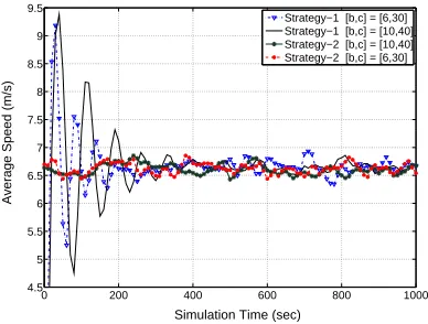
Figure 2.6 Average speed vs. simulation time. . . 46
Figure 2.7 Average speed vs. phase duration time. . . 47
Figure 2.8 Distance and trace length. . . 48
Figure 2.9 Top-view of node distribution of RWP model and SMS model. . . 49
Figure 2.10 Link performance comparison between the RWP and the SMS Model. . . 53
Figure 2.11 Connectivity performance comparison between the RWP and the SMS Model . . . 54
Figure 2.12 Routing performance comparison between the RWP and the SMS Model. . . 56
Figure 2.13 Group mobility with SMS model. . . 58
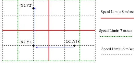
Figure 2.14 Use SMS model in a Manhattan-like area. . . 58
Figure 2.15 Different domain intervals ofK. . . 61
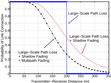
Figure 3.1 Probability of link connection between two nodes, where path loss exponentξ= 3, shadow fadingσs= 5dB, and multi-path fading is3dB. . . 71
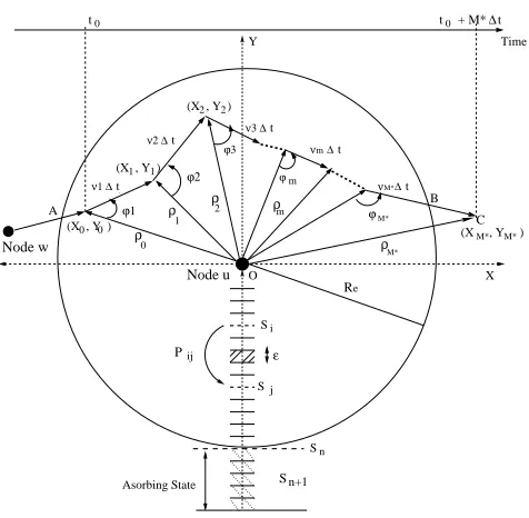
Figure 3.3 Relative movement trajectory of node-pair (u, w). . . 78
Figure 3.4 Rayleigh distribution approximation of the relative speed. . . 78
Figure 3.5 Approximation ofPij with respect toε. . . 81
Figure 3.6 Link lifetime distribution. . . 84
Figure 3.7 Stochastic properties of link lifetime. . . 86
Figure 3.8 Residual link lifetime: analytical and simulation results. . . 87
Figure 3.9 Derivation of average link arrival rateλ. . . 89
Figure 3.10 Node mobility and ETR effects on average link arrival rate. . . 90
Figure 3.11 PMF and PDF of path Lifetime. . . 93
Figure 3.12 Average number of neighbors per node according to node speedV¯ and ETR. . . 95
Figure 3.13 Effective transmission range and node mobility impacts on AODV routing perfor-mance. . . 96
Figure 4.1 Separated power-law and exponential behavior of cutoff power-law. . . 108
Figure 4.2 Human moving domain size vs. network domain size. . . 108
Figure 4.3 The mixed power-law and exponential behavior in the cutoff power-law distribu-tion. . . 111
Figure 4.4 Example of an extracted trip. . . 113
Figure 4.5 The CCDF of pause time in Campus dataset. . . 116
Figure 4.6 The CCDF of trip displacement in three dataset. . . 117
Figure 4.7 Continuous time task mobility (CTDM) model. . . 120
Figure 4.8 The CCDF of aggregated task time. . . 121
Figure 4.9 Ambivalent diffusive behavior. . . 126
Figure 4.10 Inter-meeting time upon human diffusive rater. . . 129
Figure 4.11 Link lifetime upon human diffusive rater. . . 130
Figure 4.13 Cutoff power law approximation and validation. . . 135
Figure 4.14 Cutcoff power-law vs. power-law effects on inter-meeting time. . . 136
Figure 5.1 Example of human social moving patterns. . . 145
Figure 5.2 Example of100task location sites in a network delimited by the Voronoi decom-position. . . 146
Figure 5.3 Case study of user pair correlation. . . 155
Figure 5.4 Weighted and unweighted clustering coefficient. . . 159
Figure 5.5 Example of specifying group head based on physical locations of 11 users. . . 169
Figure 5.6 Weighted edge clustering coefficient comparison. . . 174
Figure 5.7 Example of group evolution degree variation with time. . . 177
Figure 5.8 Node switch between two groups. . . 180
Figure 5.9 Operation of group initialization algorithm. . . 181
Chapter 1
Introduction
1.1
Motivation
Wireless technologies have eabled freedom of mobility by releasing the constraint of wired connections between correspondent communicating devices. Due to the advance in radio communications and a large number of demanding applications, wireless mobile multi-hop net-works have attracted tremendous attentions from both academia and industry in the past decade. A wireless mobile multi-hop network, such as a mobile ad hoc network (MANET), is an infrastruc-tureless wireless network, where all nodes equipped with radio transceivers are capable to move and communicate via radio channels. In MANETs, each node may operate not only as a host but also as a mobile router for discovering and maintaining routes to other mobile nodes. Owing to the limited transmission range, an end-to-end communication in MANETs is carried out dynamically through a number of intermediate relay nodes, which is thus called multi-hop forwarding. The goal of an MANET is to provide a rapidly and easily deployable means of interconnection between mo-bile nodes, which rely on no fixed infrastructures. Hence, MANET promises to bring the vision of ubiquitous connectivity and pervasive network coverage into reality. Motivated by the readily deployable and self-organizing nature of MANET, imminent applications are expected to be widely used in military (e.g., tactical communication in the battlefield), civilian (eg., electronic classrooms, convention centers and construction cites), law enforcement (e.g., crowd control, search and rescue), and disaster recovery (e.g., fire, flood and earthquake recovery) [1].
rely on a multi-hop fashion, the path failures occur when the links incident to the paths become unavailable. Path failures require immediate response for routing protocols to discover and update new routes [2]. However, frequent routing update messages may incur a high signaling overhead [3, 4] and energy consumption among ad hoc nodes, which seriously deteriorate the utilization of the scarce network resource [5]. Furthermore, due to path failures, excessive transmission delay, packets loss and limited throughput can dramatically degrade the performance in MANETs [6, 2]. These constraints make it much difficult to fulfill the requirement of Quality of Service (QoS)-aware applications such as multimedia transmission and collaborative computing in MANETs [7]. Hence, the performance of the potential applications of MANETs will degrade dramatically as the increase of path failures caused by node mobility [8, 9]. Therefore, compared to traditional wired networks, node mobility is a critical factor to the system performance of MANETs.
Since node mobility plays a significant role on MANET performance, understanding user moving behaviors and associated mobility patterns is essential to routing protocol design, applica-tions planning and system performance evaluation. Ideally, node mobility should be studied through existing trace files of mobile users in MANETs, such as human traces [10, 11, 12] and vehicle traces [13]. However, MANETs have not been implemented and deployed on a large-scale yet, the lack of mobility trace files from real-life applications becomes a main hurdle for characterizing realistic mobility patterns. Consequently, the mobility modeling in MAENTs has been an interesting topic because it provides a fundamental supporting tool for simulation and analysis of mobility based research issues [14, 5, 9].
node’s moving behavior have been proposed [9]. However, compared with the existing MANET studies upon random mobility models, little work has been done through temporal mobility models. In order to correctly evaluate the MANET performance, people are motivated to revisit analytical and simulation results on MANETs by applying temporal mobility models. In particular, as we discussed above, the link properties such as link lifetime directly manifest MANET performance while they are very sensitive to the user mobility mobility patterns. It is desirable to study the link properties and their correspondent impacts on MANET performance upon temporal models. Furthermore, as humans’ moving behaviors are regulated by their associated societal duties, in a practical MANET, mobile users may either move individually or in a group manner. Because the mobile wireless devices are generally attached to humans, the human mobility directly affects the properties of contact-based metrics, such as contact time and inter-contact time, and there in the routing performance in mobile ad hoc networks (MANETs) [13, 22, 23]. Therefore, a fundamental study of human mobility and its impact on the link level dynamics of mobile devices can greatly benefit the routing design and network performance analysis [14, 13, 22, 23]. In addition, due to the social correlation between humans, mobile users often move in a group way in MANETs. Given a higher correlation degree between mobile users inside a group, the contact time between group members can be much longer than a random node pair, therein the routing performance based on group mobility can be increased. On the other hand, frequent group structure variations according to member leaving and join events in groups can dramatically increase the routing maintenance cost and waste the limit bandwidth resource, therein degrade the network performance. Therefore, un-derstanding the coherence level of group structure and group stability is a key point to characterize the group evolution process, in which the number of group members vary with time and therein, the group mobility impact on the routing performance in MANETs [24, 25].
User Mobility and its Impact on Multi-hop Wireless Networks”. Specifically, we categorize our research objectives into four topics which are discussed next regarding the current works and chal-lenges, respectively.
1.2
Research Objectives
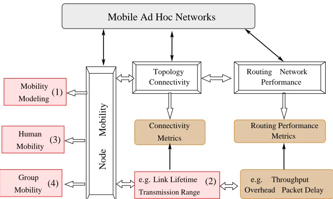
In this section, we summarize our research objectives on mobility related issues in MANETs which we aim to achieve during the course of doctoral study. Specifically, Figure 1.1 illustrates the inter-dependence of our four topics of node mobility and the overall impacts on the performance of MANETs. In this doctoral research, we first study mobility modeling, where we design a sound mobility model which not only effectively mimics transient moving behaviors of ad hoc nodes in real environments but also achieves the necessary stationary properties for proper analysis and sim-ulations. As shown in Figure 1.1, node mobility directly impacts the MANET link properties, which further influences the correspondent network connectivity and routing performance. In addition, we find that MANET link performance is influenced by the joint effects of radio channel environments and node mobility. Hence by applying the results from our first work, we want to address the un-known link properties upon these two joint effects in the second work. Further, as almost all the applications in MANETs are tightly coupled with the human daily activities, we move forward to study node mobility in the third work by investigating human mobility according to our collected GPS traces. And then, we analyze the join temporal-spatial human mobility impact on the property of inter-meeting time. Finally, we notice that practical MANET applications often require a group of users to execute a common task inside the network. Based on our results and understanding of individual node mobility, we target the study of group mobility in our fourth work. Specifically, we study the group correlation degree between mobile users based on human social correlation and similarity of nodes’ movement and their physical distance. And then, we investigate the unknown properties of group structures and group stability for characterizing the group evolution behaviors in MANETs.
In summary, the following four areas are investigated:
• Individual node mobility modeling, steady state analysis, and applications, which is our first Ph.D. topic indexed with (1) in Figure 1.1.
Node
Mobility
Mobile Ad Hoc Networks
Routing Performance Metrics Routing Network
Performance Topology
Connectivity
Connectivity
Metrics Mobility
Modeling
Human
Mobility
Group
Mobility Overhead Packet Delay
Throughput e.g.
Transmission Range
e.g. Link Lifetime
(1)
(2) (3)
(4)
Figure 1.1: Inter-dependence of node mobility with related topics and the impact on MANET performance.
which is our second doctoral study indexed with (2) in Figure 1.1.
• Empirical study of human mobility patterns in spatial-temporal domains, and Stochastic anal-ysis on their impact on inter-meeting time which is the third Ph.D. topic indexed with (3) in Figure 1.1.
• Group mobility properties analysis and applications, with is the fourth topic of this doctoral study indexed with (4) in Figure 1.1.
1.2.1 Mobility Modeling of MANETs
model has non-uniform spatial node distribution at steady state, with the maximum node density in the middle of simulation region given that initial state is uniform distribution. In [29], the authors showed that if a mobility model fails to provide a steady state of average speed, the system evalu-ation would be misleading and vary dramatically with time. Moreover, the model cannot provide appropriate solution for theoretical analysis. Corresponding to the essence of stable average speed, the virtue of uniform node distribution is two-fold. First, it is especially useful in theoretical studies, in that a system metric of interest, for example network throughput, can be properly calculated and understood without considering otherwise the undesired influence of non-uniform node distribution induced by mobility models [5, 26]. Furthermore, the majority of existing simulation and analytical studies of MANETs assume that mobile users are uniformly distributed in a network. Therefore, the mobility model with steady state uniform node distribution can accurately reflect the analysis and simulation results. In addition, as discussed in previous section, the unrealistic moving behaviors in existing random mobility models including RWP model, can mislead the results of analysis and simulations for MANETs [17, 18, 19, 20, 21].
As an effort to address the problem of unrealistic movements and to provide desirable sta-tionary moving behaviors, mobility models that consider the correlation of node’s moving behavior are desirable. Noticing that existing mobility models do not satisfy these necessary requirements, in our first research work, we are motivated to design a new mobility model, named Semi-Markov Smooth (SMS) model, that can abide by the physical law of moving objects to avoid abrupt moving behaviors, and can provide a microscopic view of mobility such that node mobility is controllable and adaptive to different network environments. Furthermore, the model is expected to be mathe-matical tractable and bear the desired steady state properties including stable average speed [29] and uniform spatial node distribution [20], so that it can be used to correctly evaluate the performance of MANETs. The detailed design patterns and analysis of our proposed mobility model are elaborated in Chapter 2.
1.2.2 Joint Effects of Radio Channels and Node Mobility on Link Dynamics
of QoS guaranteed services in MANETs. Therefore, understanding the nature of link dynamics is essential to design mobility-resilient MANETs[30, 9, 26], maximize routing performance[31, 2], optimize topology control[32, 33, 34], and achieve the desired network performance[5, 7].
Besides the node mobility, the time-varying radio environment is another inherent prop-erty of MANETs. Specifically, a received signal of mobile nodes is influenced by three fading effects: large-scale, multipath, and shadowing [35], so that the radio channel (link) status may vary greatly in different wireless environments, even the node-pair distance is same. In addition, we notice that the link performance degrades dramatically as the increase of the fadings in the radio channel. It turns out that the link performance is very sensitive to both node mobility and radio channel characteristics, which is considered as the major difference from the communication in wired networks. Therefore, because of the inherent nature of MANETs, it is insufficient to analyze the link dynamics from the single effect of node mobility. In other words, it is necessary to study MANET link properties upon the joint effects of node mobility and radio channels.
There has been a large number of studies on the effect of node mobility on link dynamics, such as link lifetime [36, 5, 26, 37, 38], link change rate [26], link residual time and link availability [39, 36, 40, 26, 37]. However, little effort has been done to analyze the link dynamics from the joint effects perspective. Specifically, existing studies on link dynamics are mainly focused on random mobility models such as Random Walk (RW) mobility model [41] and a fixed transmission range, which could bring three limitations on the obtained results. First, random models frequently gen-erate abrupt moving behaviors such as sudden stop and sharp turn which are not in comply with smooth motions in real world [42, 41]. Moreover, as mobile nodes do not change velocity within each time epoch, random mobility models cannot describe smooth speed and direction transition in one movement, which however is very common in real moving scenarios. Second, the transmis-sion range of a mobile node in reality varies dynamically due to the time-varying wireless radio environment [32, 33, 43]. In addition, the study in [44] suggested the time scale used to describe node mobility should be less than the time scale for capturing the significant channel variability, which implies smooth mobility models described in small time scale, for instance, the SMS model proposed in our first work, are more preferable for analyzing link properties.
link lifetime, link residual time, and link change rate. Moreover, we are interested in finding the weight of impacts on link performance between node mobility and radio environments according to diversified MANET scenarios. The details our this work will be represented in Chapter 3.
1.2.3 Diffusive Properties of Human Mobility and Its Impact on Contact-based Met-rics
In fact, majority of mobile nodes in a typical wireless multi-hop network is expected to be either pedestrians carrying wireless enabled devices or vehicles containing humans which support wireless communications. As a result, the human mobility directly affects the link level dynamics between mobile wireless devices, which are characterized by the contact-based metrics, such as contact time and inter-contact time, in mobile ad hoc networks (MANETs) [14, 13, 22, 23]. For instance, the contact time (also called link lifetime) is counted for the time duration when two mobile users have a directly connected link. As a link often disconnects when a mobile user moves outside the transmission range of the other user, the inter-contact time (also called inter-meeting time) is defined as the time period between two consecutive link connections of two mobile users. Therefore, the deep understanding of human mobility pattern and its implications is indispensable to study the properties of contact-based metrics, which in turn, are critical to routing protocol design and network planning.
[49, 50, 52]. The main challenge is that it is not easy to specify the accurate user location and trip movements in these traces. Fortunately, Global Positioning System (GPS) enabled devices have become affordable and have been widely used since recent years. Thus, people start to carefully study the human mobility traces by GPS loggers since 2005. Specifically, the research works focus on human mobility according to spatial effects, such as trip length [56, 57, 22], or temporal effects such as inter-meeting time [12, 55] and pause time [54, 22]. However, as human mobility patterns are influenced by complex social and cultural contexts, it is very difficult to generalize the human mobility patterns upon diversified locations and times. Consequently, there are still many open questions unsolved. For example, what are the inherent properties of human mobility? In other words, without specifying human mobility pattens qualitatively and quantitatively, it is unlikely to accurately analyze the impact of human mobility on MANET performance.
In [56, 57], the authors showed that human mobility patterns and moving capability can be effectively manifested by his/her diffusive capability (order)r. Nevertheless, it is still not clear how to specify the diffusive orderrwith respect to different human diffusive behaviors and what is the fundamental human behavior rules with their societal duties in reality. Therefore, the importance and yet limitations of existing research on human mobility strongly motivate us to investigate the human mobility patterns, especially for human diffusive properties, from both spatial and temporal perspectives. To proceed, we collected human GPS traces and record their daily activities for three months (over a thousand hours), upon which we expect to understand, interpret and model the human diffusive behaviors. Furthermore, it has been suggested that human mobility can greatly affect the properties of contact-based metrics in MANETs [12, 55, 54, 22]. Hence, we are motivated to investigate the relation between human diffusive mobility patterns and the property of inter-meeting time in multi-hop wireless networks. Our detailed work is elaborated in Chapter 4.
1.2.4 Inherent Properties of Group Mobility for Mobile Wireless Networks
to execute a mission which is attacking the enemies’ target, a troop of soldiers move following their command leader in a tactic way. Second, it can often be observed as a location-oriented group mobility in MANETs, in which a number of users move together toward the same destination. For instance, a team of visitors move follow a tour-guider for the same masterpiece of interest in a museum. Third, mobile users could be categorized into groups according to their organizations. For example, on a disaster scene, firefighters, policemen and doctors join three groups for differ-ent rescue operations. As practical MANET applications are often involved with group mobility, a number of research works have been elaborated upon the impact of group mobility in MANETs [58, 61, 62, 63, 64, 65]. Recent studies demonstrated that group mobility can benefit the overall network performance, for instance, improving the routing efficiency [24]. Especially, as the size of the network increases, a flat network structure will encounter the scalability problem, which is more difficult to handle in MANETs due to node mobility. If considering each group as a cluster, to enhance scalability, hierarchy routing based on clusters is often applied for a large scale net-work [2, 64]. In addition, group mobility can improve the efficiency of location management by designing a hierarchical location database architecture upon groups [66] and improve topology con-trol management in MANETs [67]. Compared with the topology changes in a network composed of individual nodes, the network topology is more robust to nodes moving in groups because the correlation of mobile nodes in a group reduces the potential of path failures.
Furthermore, we observed that in reality, a general group in a network typically expe-riences the birth-to-death process including group initiation, group evolution and group member disperse in sequence. However, it is still unknown how to capture and predict the detailed group evolution behaviors in mobile wireless networks. As an advanced study, we aim to investigate the group evolution properties based on the analytical results obtained in the first phase of this research. In particular, we want to find out under which conditions the group size and structure can evolve in the network? In addition, we notice that almost all the existing group mobility models have two limitations on describing group moving behaviors. First, existing group mobility models, such as RPGM model, did not capture the group evolution process, there is no node join and node switch event occurs during the entire group movement. Second, the group did not deform during the entire simulation. Thus, there is no birth-to-death group process during the simulation. Hence, existing group mobility models may not be consistent with the group moving behaviors in reality. In or-der to mimic both birth-to-death group process and group evolution behaviors in MANETs, we are motivated to apply the metrics studied in this work to design a novel birth-to-death group mobility model. The detailed representation of this work is in Chapter 5.
1.3
Research Challenges
During the course of this doctoral research, there are many non-trivial challenges we have to tackle with. In this section, we discuss the major challenges which are categorized into the following groups: radio environment issues, mobility model design issues, human spatial and
temporal moving trace collection, diversified human trace dataset requirements, and societal and
working environment effects.
node distribution, which lead to overoptimistic evaluations on MANET link and routing per-formance. Furthermore, recent studies shows that the finite border of simulation area causes the power-law – exponential decay issues on the CCDF of inter-meeting time and trip dis-placement. Hence, design an appropriate synthetic mobility model which can not only avoid the unrealistic moving behaviors by complying with the physical law of moving objects in reality but also provide tractable analysis is a challenge issue. More important, the designed model should achieve the desirable stationary moving behaviors while reducing or avoiding the undesired border effect, which makes it more difficult to the design of mobility models. Moreover, people already observed that the network and routing performance is very sensitive to the node mobility patterns. How to design a unified mobility model which can be flexibly and easily controlled to diverse user moving behaviors is not trivial.
• Small Time Scale of Link Variations in Radio environment: In general, a received signal of mobile nodes is influenced by three fading effects: large-scale, multipath, and shadowing. Hence, the MANET link status may vary greatly in different wireless environments, even the node-pair distance is same. Due to the limited power consumptions, the transmission range of a mobile node is dynamic according to the time-varying wireless radio environment, which in turn varies the link status between neighboring nodes and the network topology. In consequence, it is really difficult to analyze network topology changes, link dynamics and routing performance in the presence of complex node mobility and the unpredicted radio environments. More specific, the main challenge here is how to tackle the small time scale of radio link variations and random node mobility together on studying the link performance of MANETs.
our doctoral research, which necessarily requires the diversified human traces having different scales of human diffusive (moving) domains. However, most available human trace datatsets are campus-wide traces. This imposes a big challenge on collecting different empirical human traces with different scales of human moving domain size.
• Societal and working environment effects: Human mobility is closely coupled with the demanding MANET applications. It has been observed that human mobility patterns are in-fluenced by complex social and cultural contexts. The human moving behaviors are affiliated with their duties and working patterns in a certain territory. And the affiliation varies accord-ing to different duties in different territories. Particularly for group user movaccord-ing behaviors, the mission-oriented group mobility is often observed in MANET applications. For example, putting out a fire is the common mission of all firefighters on a disaster scene, where they move closely in a group to execute the task. However, humans are often involved in very complicated societal environments, and the social status of a single person such as a worker, a student, and a shopper, frequently changes upon different spatial-temporal domains. How to characterize the individual and group human mobility patterns is very challenging. Espe-cially for group movements in MANETs, how to specify the group coherence and project the group evolution process under different social and working duties of mobile users is a very challenging issue.
1.4
Contributions
In summary, the main contributions of this Ph.D. study is to provide a deep understanding of node mobility behaviors and its impacts to the system design, routing optimization, and perfor-mance analysis in mobile wireless networks. To achieve this goal, we studied four mobility related research topics step by step in this doctoral study. As shown below, we list our major contributions obtained by far according to each research topic.
speed of SMS model is stable with simulation time, hence avoid the well-known speed decay problem of Random Waypoint mobility model. We further showed that the SMS model al-ways maintains the uniform node distribution of mobile nodes with time. Through stochastic analysis, we claimed that this model unifies many good features for analysis and simulations of mobile networks. First, it is smooth and steady because there is no speed decay problem for arbitrary starting speed, while maintaining uniform spatial node distribution regardless of node placement. Second, it can be easily and flexibly applied for simulating node mobility in wireless networks. It cal also adapt to different network environments such as group mobility and geographic constraints. To demonstrate the impact of this model, we evaluate the effect of this model on distribution of relative speed, link lifetime between neighboring nodes, and average node degree by ns-2 simulations. This proposed unified mobility model provides a fundamental support for our second research topic.
• Second, we took a new modeling approach that captures the dynamics of radio channels and node movements in small-scale upon microscopic mobility models, such as the SMS model. Specifically, a distance transition probability matrix is designed in order to describe the joint effects of dynamic transmission range due to radio channel fading and relative distance of a node-pair resulting from random movements. We found that the PDF of link lifetime can be approximated by an exponential distribution with parameter characterized by the ratio of average node speedV¯ to effective transmission range Re. And the probability distribution
function of path lifetime can be effectively approximated by an exponential distribution for any k-hop path, with parameter of λk
P, which is the summation of exponential parameters
of each link along the path. Moreover, we study the PMF of path lifetime which has an immediate impact on end-to-end communications in multi-hop wireless networks in that each path is composed of multiple links. To further understand the implication of link properties, analytical results are used to investigate the upper bound of network connectivity and the associated network performance is evaluated by extensive simulations. We showed that for a large dense network, its network connectivity is bounded by the average node degree, which is equivalent to the multiplication between the average link arrival rate and the average link lifetime.
displacement of human mobility exhibit a cutoff-power distribution. In particular, the cutoff point, defined as characteristic distanceDc, in the distribution of trip displacement increases
as the human moving domain size increases. Then, we study the joint temporal-spatial effects of pause time and trip displacement on the inter-meeting time of mobile users, when both pause time and trip displacement are characterized by the power-law head in the distribution. We find that the interaction between trip displacement and pause time on human mobility can be manifested by the human diffusive movement patterns [56], which is further charac-terized by his/her diffusive capability (rate) r. Then, by studying the scaling law of human diffusive rate, we show that when the power-law head characterizes both pause time and trip displacement with the power-law coefficientsαandβ, respectively, the human diffusive rate r is, r = 2α/β, where0 < α < 1and 0 < β < 2. We further investigate the mixed be-haviors of power-law head and exponential tail of a cutoff power-law upon the analysis on empirical human trace datasets with different levels of moving domain sizes. Then, we pro-pose an approximated cutoff power-law distribution, which is featured by a parameter tuple (the power-law coefficient and cutoff point), for instance, (α, Tc) and (β, Dc), for pause time
and trip displacement, respectively. The approximated cutoff power-law distribution exhibits a close fit with the empirical results from trace files. Finally, with simulation results based on different human diffusive rates, we demonstrate that the human diffusive ratercan effec-tively characterize the property of contact-based metrics, especially for inter-meeting time, in MANETs. Specifically, we found that superdiffuive rater >1leads to the longest power-law head, while the subdffusive rater < 1results in the shortest power-law head in the distri-bution of inter-meeting time. Thus, the higher the diffusive rate is, the longer the power-law head is in the distribution of inter-meeting time.
We observed that a general group in MANETs typically experiences a birth-to-death process including group initiation, group evolution with member join and leave and group deforma-tion in sequence. Then based on the user-pair correladeforma-tion, we developed a new metric, called node connectness to characterize the stability level of inter-connections among the node with its group neighbors. And this stability level can reflect the potential node switch and detach event in a group. In addition, we study the routing impact of a node regarding its group struc-ture, which is based on the node neighbors’ degree metric. With this metric, we can improve the routing throughput and bandwidth utilization for multicast traffic inside a group. The over-all network routing performance is affected by the group evolution behaviors. Therein, we provided a metric, named group evolution degree, to characterize the group member variation degree due to node detach during the group evolution process. Furthermore, we investigate the condition for group member switching between groups. Finally, we propose a novel birth-to-death group mobility model for both analytical and simulation studies in MANETs. As a case study of routing protocol evaluation, we demonstrate that the widely applied RPGM model stresses AODV much less than the proposed BDGM model, since RPGM model does not take the group birth-to-death evolution behaviors into account, and could bring biased results for group mobility based study.
Chapter 2
Design and Study A Unified Mobility
Model for Analysis and Simulation of
Mobile Wireless Networks
In this chapter, we present the first research topic in this doctoral study, which is to design and analyze a novel Semi-Markov Smooth Mobility (SMS) model for mobile wireless networks. We first motivate this study and review some related works in Chapter 2.1. Next, we describe the detail movement patterns of the proposed SMS mobility model in Chapter 2.2. Then, we analyze the Transient stochastic properties of SMS model regarding the major mobility metrics of movement duration, speed, and trace length in Chapter 2.3. After that we investigate both the transient and the steady state properties of the SMS model in Chapter 2.4 and Chapter 2.5, respectively. In Chapter 2.6, we validate the analysis of SMS steady state properties with simulations. The impacts and applications of SMS model in mobile wireless networks are elaborated in Chapter 2.7. Finally, we summarize our main contributions of the first work in Chapter 2.8.
2.1
Motivation and Related Work
mobile ad hoc networks. There are many mobility models which have been well studied in survey papers [15, 14, 9] which are focused on synthetic models, except few experimental studies [10, 11]. The challenge in designing mobility models is the trade-off between model efficiency and accuracy. Due to easy analysis and simple implementation, random mobility models, in which each mobile node moves without constraint on its velocity, time period and destination, are most widely used [9]. For example, random walk (RW) model was originally proposed to emulate the unpre-dictable movements of particles in physics, also known as Brownian motion [9]. Compared to the RW model, Random Waypoint (RWP) model [16] is often used to evaluate the performance of mo-bile ad hoc networks (MANETs) due to its simplicity. However, two flaws have been found in its stationary behavior. First, Yoon showed that the average node speed of RWP model decreases over time [17]. Second, Bettstetter [18] and Blough et al. [28] respectively observed that RWP model has non-uniform spatial node distribution at steady state, with the maximum node density in the middle of simulation region given that initial state is uniform distribution. This implies that analysis and simulations based on RWP model may generate misleading results. To overcome the non-uniform spatial node distribution problem in RWP model, Nain and Towsley recently showed that random
direction (RD) model [76] with warp or reflection on the border has uniformly distributed user
po-sition and direction in [20]. Recently, Boudec et al. proposed a generic random mobility model, called Random Trip (RT) model, which covers RW, RWP and RD models, as well as their variants [19].
Random mobility models describe the mobility pattern in a macroscopic level, that is, mobile nodes do not change speed or direction within one movement. Thus, random mobility mod-els can fit vehicular and large-scale environments. Therefore, they are insufficient to mimic the minute moving behaviors of mobile users, such as speed acceleration and smooth direction changes within one movement. The movements presented by random models are completely uncorrelated or random, thus demonstrating unrealistic moving behaviors, such as sudden stop, sudden acceler-ation, and sharp turn frequently occur during the simulation [9]. These abrupt speed and direction change events will influence the network topology change rate, which further significantly affect network performance. In consequence, the simulation results and theoretical derivations based on random mobility models may not correctly indicate the network performance and effects of system parameters.
which are called temporal models [9], such as Smooth Random (SR) model [15] and Gauss-Markov (GM) model [77]. SR model considers the smooth speed and direction transitions for mobile nodes. In the SR model, a node moves at a constant speed along a specific direction until either a speed or direction change event occurs according to independent Poisson process. In the GM model, the velocity of a mobile node at any time slot is a function of its previous velocity with a Gaussian random variable. Although both SR and GM models can be used for either cellular environments or ad hoc networks, they also have application limitations. In the SR model, because of the assump-tion of Poisson process, the uncertainty of the speed and direcassump-tion change within each movement make it difficult to evaluate network performance according to a specific node mobility requirement. Moreover, an SR movement may have new speed change during the speed transition and does not stop unless a targeting speed is specified as zero, which is not flexible for movement control. In the GM model, mobile nodes cannot travel along a straight line [14] as long as the temporal correlation (memorial) parameter is not equal to 1, and they do not stop during the simulation. However, in reality, vehicles usually move along a straight line for a period of time and mobile users always move in an intermittent way with a random pause time.
Therefore, we are motivated to design a new mobility model that can abide by the physical law of moving objects to avoid abrupt moving behaviors, and can provide a microscopic view of mobility such that node mobility is controllable and adaptive to different network environments. In summary, this model is expected to unify the desired features as follows:
1. Smooth and sound movements: A mobility model should have temporal features, i.e., a mo-bile node’s current velocity is dependent on its moving history so that smooth movements can be provided and mobile nodes should move at stable speed without the average speed decay problem [29].
2. Consistency with the physical law of a smooth motion: In order to mimic the kinetic correlation between consecutive velocities in a microscopic level, a mobility model should be consistent with the physical law of a smooth motion in which there exists acceleration to start, stable motion and deceleration to stop for controllable mobility [78, 79].
spatial node distribution at steady-state. Otherwise, the non-uniform node distribution caused by a mobility model may invoke misleading information and results [20].
4. Adaptation to diverse network application scenarios: In order to properly support rich MANET applications having complex node mobility and network environments, such as group mobility and geographic restriction, a generic mobility model which is adaptive to different mobility patterns is highly desirable.
In addition, compared to the design and simulation studies of mobility modeling in ex-isting literatures, there exists very limited analysis works of mobility models such as steady state analysis of node speed, direction, and node distributions. In order to fill up the gap in the design of microscopic mobility models and the analysis of their steady state properties, we are further mo-tivated to analyze the steady state properties of the proposed SMS model, considered as a unified mobility model, which are essential to understand the system performance and topology dynamics of MANETs.
2.2
A Unified Mobility Model: Semi-Markov Smooth (SMS) Model
In this section, we present a novel mobility model, Semi-Markov Smooth (SMS) model with detailed mobility patterns. Specifically, within one movement, we elaborate when and how an SMS node changes its speed and direction; how the node accelerates and decelerates the speed; and how strong the temporal correlation is during the speed and direction change. By answering these questions, the moving behaviors of mobile nodes can be deeply understood and well manifested by the proposed model. Further, we describe the stochastic process of the SMS model. We consider it as a renewal process with respect to consecutive SMS movements and regard it as a semi-Markov process in the study of iterative phases transition.
2.2.1 Model Description
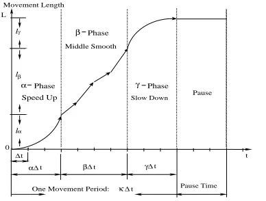
Slow Down phase, and Pause phase. Throughout this disertation, we define one SMS movement or
movement duration as the time period that a node travels from the starting point to its next
posi-tion that the node stops moving. Each movement is quantized intoKequidistant time steps, where
K ∈ Z. The time interval between two consecutive time steps is denoted as ∆t(sec). The SMS
model is an entity model which determines the mobility pattern of each user individually, which is designed with the following assumptions:
• All mobile nodes move independently from others and have the identical stochastic properties.
• For any mobile nodes, every SMS movement has identical stochastic properties.
• Within each SMS movement, a mobile node’s velocity at current time step is dependent on its moving history.
Here, the first two assumptions are similar to the random mobility models for better sup-porting theoretical studies as well system performance evaluation of MANETs. To be distinguished from random mobility models, the third assumption of the SMS model is especially used for de-scribing microscopic smooth nodal movements. Next, we describe the SMS model based on the single user mobility. The implementation for group mobility and geographic constraints will be explained in Chapter 2.7.
Speed Up Phase (α–Phase)
For every movement, an object needs to accelerate its speed before reaching a stable speed. In this phase, the movement pattern of an SMS node is exploited from what is defined in SR model [15]. Thus, the first phase of a movement is called Speed up α–Phase, which covers the time interval [t0, tα] = [t0, t0 +α∆t]. At initial time t0 of a movement, the node randomly
selects a target speedvα ∈ [vmin, vmax], a target directionφα ∈ [0,2π], and the total number of
time steps αfor the speed up phase. α ∈ Zand is selected in the range of[αmin, αmax]. These
three random variables are independently uniformly distributed. Note that αmin and αmax imply
the physical speed-up capabilities of the node. For instance, whenαis selected close toαmax, the
transition time is long , but the degree of temporal correlation is strong.
In reality, an object typically accelerates the speed along a straight line. Thus, the direction φαdoes not change during this phase. To avoid sudden speed change, the node will evenly accelerate
ending speed ofα–phase, i.e.,v(tα) = vα. Hence, the mobility pattern in speed upα–phase is
represented by a triplet(α, vα, φα). The acceleration rate atα–phase,aα, can be obtained by
aα=
vα−v(t0)
tα−t0
= vα
α∆t. (2.1)
An example of speed change inα-phase is shown in Figure 2.1(a), where the node speed increases evenly step by step and reaches the target speedvαby the end of this phase.
Middle Smooth Phase (β–Phase)
After the initial acceleration, a moving object will have a smooth movement, even though moving speed and direction may change. Accordingly, once the node transits intoβ-phase at time tα, the node randomly selectsβtime steps and moves intoβ–phase. During time interval(tα, tβ] =
(tα, tα +β∆t], where β ∈ Zis uniformly distributed over [βmin, βmax]. As a succeeding phase
ofα–phase, the initial value of speedv0 and direction φ0 inβ–phase are vα and φα, respectively.
The speed and direction during β–phase then change on the basis ofvα andφαat a memory level
parameterζ, which ranges over[0,1]and is constant for both speed and direction at each time step. Thus, by adjusting parameterζ, we can easily control the degree of temporal correlation of velocity between two consecutive steps. For example, let us assume that the standard deviationσv andσφ
are1, which implies that the speed or direction difference between two consecutive time steps is less than 1m/sor 1 rad withinβ–phase. Through simulations, we find that this granularity is sufficient to describe user mobility.
Then the step speed (i.e., speed at a time step) and step direction (i.e., direction at a time step) at thejthtime step for an SMS node inβ–phase are presented by:
vj = ζvj−1+ (1−ζ)vα+
p
1−ζ2Ve
j−1
= ζjv0+ (1−ζj)vα+
p
1−ζ2
j−1
X
m=0
ζj−m−1Vem
= vα+
p
1−ζ2
j−1
X
m=0
ζj−m−1Vem, (2.2)
and
φj = ζφj−1+ (1−ζ)φα+
p
1−ζ2φe
j−1
= φα+
p
1−ζ2
j−1
X
m=0
whereVej and φej are two stationary Gaussian random variables with zero mean and unit variance,
independent from V, andφj, respectively. By substitutingβ forj into (2.2) and (2.3), the ending
step speedvβand ending step directionφβ ofβ–phase are obtained as:
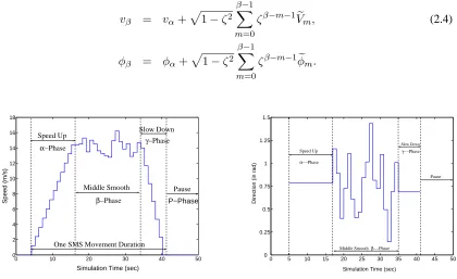
vβ = vα+
p
1−ζ2
βX−1
m=0
ζβ−m−1Vem, (2.4)
φβ = φα+
p
1−ζ2
β−1
X
m=0
ζβ−m−1φem.
0 10 20 30 40 50 0 2 4 6 8 10 12 14 16 18
Simulation Time (sec)
Speed (m/s)
Speed Up Slow Down
Middle Smooth Pause
α−Phase
β−Phase
γ−Phase
One SMS Movement Duration
P−Phase
(a) Speed vs. time in one SMS movement.
0 5 10 15 20 25 30 35 40 45 50 0 0.25 0.5 0.75 1 1.25 1.5
Simulation Time (sec)
Direction (in rad)
Speed Up
α−−Phase
Middle Smoothβ−−Phase
Slow Down γ−−Phase
Pause
(b) Direction vs. time in one SMS movement.
Figure 2.1: An example of speed and direction transition in one SMS movement. Given (2.2) and (2.3), the mobility pattern inβ-phase is represented by a quartet
(β, vα, φα, ζ). As shown in Figure 2.1(a), node speed fluctuates around the speedvα achieved at
the end ofα–phase in each step ofβ-phase. In an SMS movement,β-phase is the main moving phase, which characterizes the mobility level and direction for a node during the entire movement.
Slow Down Phase (γ–Phase)
According to the physical law of motion, every moving object needs to reduce its speed to zero before a full stop. In order to avoid the sudden stop event happening in the SMS model, we consider that the SMS node experiences a slow down phase to end one movement. In detail, once the node transits into γ–Phase, i.e., slow down phase, at timetβ, it randomly selects γ time steps
interval(tβ, tγ] = (tβ, tβ+γ∆t], whereγ ∈Zand is uniformly distributed over[γmin, γmax]. The
SMS node will evenly decelerate its speed fromvβ tovγ = 0. The rightmost part in Figure 2.1(a)
shows an example of speed change inγ–phase. In reality, a moving object typically decelerates the speed along a straight line before a full stop. Thus, the direction φγ does not change during the
γ–phase. In order to avoid the sharp turn event happening during the phase transition, φγ and φβ
are correlated. Specifically, φγ is obtained from (2.3), by substituting β forj−1. At the end of
γ–phase, i.e.,tγ, a mobile node stops at the destination position of its current movement. Thus, the
mobility pattern inγ–Phase is represented by a triplet(γ, vβ, φγ). The deceleration rateaγis given
by:
aγ=
vγ−vβ
tγ−tβ
=− vβ
γ∆t. (2.5)
Figure 2.1(a) shows an example of speed vs. time during one SMS movement, which contains a total number ofK = 37small consecutive steps, whereα–phase contains12time steps, β–phase includes 18 time steps, and γ–phase consists of 7 time steps. After each movement, a mobile node may stay for a random pause timeTp. Correspondingly, Figure 2.1(b) illustrates the
node’s direction behavior of the same SMS movement. It is clear to observe that the direction is constant in bothαand γ–phase. Specifically, φα = 0.8rad andφγ = 0.68rad, respectively. And
the direction fluctuates around φα at each step inβ–phase based on (2.3). Moreover, the largest
direction transition between two consecutive time steps is 0.23π between 28th and 29th second, which means only small direction change occurs in each time step. As the difference between φα and φγ is small in this example, it implies a strong temporal correlation between consecutive
velocities for the node. Thus, the target direction φαeffectively predicts the direction of the entire
SMS movement.
2.2.2 Stochastic Process of SMS Model
Renewal Process of SMS Model
For proper nomenclature, random variables used to represent the process in SMS stochas-tic model are denoted at two levels: all random variables denoted for SMS movements are written in upper case and within each movement, all random variables denoted for trips for each time step are written in normal font. Multi-dimensional variables (e.g., random coordinates in the simulation area) are written in bold face. In the proposed model, all mobile nodes move independently from each other and have the identical stochastic properties, so that it is sufficient to focus on the study of stochastic process of the SMS model with respect to a specific node. Hence, we suppress the node index in the denotations of random variables for simplicity. The discrete-time parameter i indexes theith movement of an SMS node, wherei∈ No, andNo is denoted as a countable non-negative
integer space. The discrete-time parameter j indexes thejthtime step within one movement of an
SMS node. For discrete-time stochastic process in SMS model, all indexes are written in normal
font. For example,v(i, j)denotes node speed atjthtime step within itsithmovement.
For the rest of paper, we use the following denotations for movements and steps within each movement:
• SMS movement: Movement Duration T(i)represents the time period of the ith movement
from the beginning ofα–phase to the end of γ–phase; Movement Position P(i) represents the ending position of theith movement; andK(i) is total number of time steps of the ith movement, whereK(i) =α(i) +β(i) +γ(i).
• Steps: Step Positiond(i, j), Step Speed v(i, j), and Step Directionφ(i, j)denote the ending position, speed, and direction at thejthtime step of theithmovement, respectively.
As a new transition happens at the beginning time at each SMS movement, the movement can be regarded as a recurrent event. The movement durationT(i)represents the time between the (i−1)thand theithtransition of the SMS movement. SinceT(i)is an i.i.d. random variable, the movement of SMS model is a renewal process{N(t);t≥ 0}, whereN(t)denotes the number of renewals by timet[80]. Without considering the pause time after each movement, the time instant Siat which theithrenewal occurs, is given by :
Si=T(1) +T(2) +...+T(i), S0= 0, i∈N. (2.6)
Hence, N(t) is formally defined as N(t) , max{i : Si ≤ t}. If consider that a random pause
and theith transition of the SMS process, whereTe(i) = T(i) +Tp(i). Because Tp(i) is an i.i.d
random variable and independent fromT(i), Te(i)is also an i.i.d random variable. Therefore, the consecutive movements of SMS model is a discrete-time renewal process irrespective of pause time.
Semi-Markov Process of SMS Model
Since an SMS movement consists of three consecutive moving phases and a pause p– phase, the continuous-time SMS can be represented as an iterative four-state transition process, which is shown in Figure 2.2.
~ Tp
t t
t
Tp F (t)
Iα α ∆ Iβ β ∆ Iγ γ ∆ IP
Figure 2.2: Four-state transition process in SMS model.
LetI represent the set of phases in SMS process, then I(t)denotes the current phase of SMS process at time t, where I = {Iα, Iβ, Iγ, Ip}. Let{Z(t);t ≥ 0} denote the process which
makes transitions among four phases inIandYndenote the state of{Z(t)}at the epoch of itsnth
transition. Because the transition time between consecutive moving states in an SMS movement has a discrete uniform distribution, as shown in Figure 2.2, instead of an exponential distribution. By this argument,{Z(t)}is a semi-Markov process [81]. This is the very reason that our mobility model is called semi-Markov smooth model because it can be modeled by a semi-Markov process and it complies with the physical law with smooth movement. Accordingly, {Yn;n ∈ N} is the
four-state embedded semi-Markov chain of{Z(t)}.
We denotePs1s2 as the probability that when {Yn}enters a states1, the next state will
be entered iss2. Further, Fs1s2(t)denotes the cumulative distribution function (CDF) of the time
to make the s1 → s2 transition when the successive states are s1and s2. Let Ts1 represent the
holding-time that the process stays at states1before making a next transition. Then we useHs1(t)
to represent the CDF of holding-time at states1, which is defined as follows [81]:
Hs1(t) =
X
s2∈I
P rob{Ts1 ≤t|next states2}Ps1s2 =
X
s2∈I
According to four-state semi-Markov chain{Yn}shown in Figure 2.2, there is only
uni-directional transition between two adjacent states in SMS model, such that the state transition prob-ability Ps1s2 = 1, if and only if s1s2 ∈ {IαIβ, IβIγ, IγIp, IpIα}. Under this condition, Hs1(t)
is equal toFs1s2(t)in the SMS model. Specifically, FIαIβ(t),FIβIγ(t)and FIγIp(t)have discrete
uniform distribution, while pause timeTp can follow an arbitrary distribution, denoted by fTp(t).
Therefore, from (2.7), the probability density function (pdf) of holding-timeTs1 in SMS model is
a discrete uniform distribution when s1 6= Ip and is fTp(t) whens1 =Ip. Therefore, this
mobil-ity model follows a semi-Markov process because the pdf of state holding time is not exponential distribution for Markov process.
2.3
Stochastic Properties of SMS Model
Mobility model has a significant impact on both simulation-based and analytical-based study of wireless mobile networks. A deep understanding knowledge of the moving behaviors of this model is critical to properly configure the mobility parameters for a variety of network scenar-ios; to correctly interpret simulation results, especially for routing protocol design and evaluation; and to provide fundamental theoretical results for other mobility related analytical studies such as link and path lifetime and network connectivity analysis. Therefore, we study the stochastic prop-erties of SMS model in this section.
Although different mobility models lead to different mobility patterns, the stochastic prop-erties of movement duration, speed, and trace length (distance) are of major interests in all mobility models because they are immediate metrics to characterize a node’s movement. In fact, in every mobility model, at least two of these metrics are specified. For example, in RWP model, the mobil-ity pattern of each movement is characterized by the trace length (distance) and speed, whereas RD model combines movement duration, speed and direction together to dominate the mobility pattern. Based on the model assumption in Chapter 2.2.1, the SMS process is a renewal process, so that it is sufficient to study the stochastic properties of a single movement in SMS model by omitting the index iand use lower case j alone to identify the random variable within one SMS movement. For example,T represents the movement duration, and vj denotes the step speed at the
2.3.1 Movement Duration
In each movement, we consider the movement duration as the time period from the be-ginning of α–phase to the end of γ–phase. According to the definition of SMS model in Chap-ter 2.2.1,T = K∆tand ∆tis a constant unit value, whereK is the summation of three indepen-dent uniformly distributed random variables α,βand γ. Therefore, the duration time of one SMS movement is determined by the number of time steps Kand movement duration follows the same probability mass function (pmf) of variableK. So, we first derive the distribution of time stepsK of SMS model and then, we can find the expected movement duration, E{T}. For the simplicity of denotation, we set the range ofα,β, and γ as[Nmin, Nmax]in the remaining of the paper, i.e.,
αmin = βmin = γmin = Nmin and αmax = βmax = γmax = Nmax. The detailed derivation of
the pmf of time stepsK is shown in APPENDIX 2.9. By integrating the results of three scenarios discussed in APPENDIX 2.9, that is, we combine (2.46), (2.47), and (2.48), the pmf of time steps,
K, is obtained as:
P rob{T =k∆t}=P rob{K=k}
=
k2−6k·N
min+3k+9Nmin2 −9Nmin+2
2(Nmax−Nmin+1)3 Case 1
6k(Nmin+Nmax)−2k2−3(Nmin2 +Nmax2 +4Nmin·Nmax+Nmin−Nmax)+2
2(Nmax−Nmin+1)3 Case 2
k2−6k·N
max−3k+9Nmax2 +9Nmax+2
2(Nmax−Nmin+1)3 Case 3,
(2.8)
where in Case 1,3Nmin ≤k≤2Nmin+Nmax; in Case 2,2Nmin+Nmax ≤k≤2Nmax+Nmin;
and in Case 3,2Nmax +Nmin ≤ k ≤ 3Nmax. In addition, as the duration time in each moving
phase follows uniform distribution and is assumed to be equal over the range [Nmin, Nmax], the
expected value of Movement DurationT can be derived as follows:
E{T}= (E{α}+E{β}+E{γ})∆t= 3∆t
2 (Nmin+Nmax). (2.9) Since∆tis a constant unit time, in order to simplify the presentation,∆tis normalized to unity in the rest of the paper.
20 40 60 80 100 120 0
0.005 0.01 0.015 0.02 0.025 0.03 0.035
One SMS Movement Duration Time
PMF
[b,c]=[6,30] [b,c]=[10,40]
(a) PMF of one SMS movement duration.
20 40 60 80 100 120
0 0.1 0.2 0.3 0.4 0.5 0.6 0.7 0.8 0.9 1
One SMS Movement Duration Time
CDF
[b,c] =[6,30] [b,c] = [10,40]
(b) CDF of one SMS movement duration.
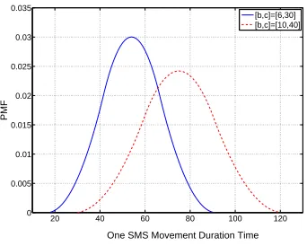
Figure 2.3: The PMF and CDF of one SMS movement duration according to different phase duration ranges.
As each phase duration in the SMS movement has a discrete uniform distribution, from (2.9), the average movement duration is54seconds when[Nmin, Nmax] = [6,30]seconds, and is75seconds
when [Nmin, Nmax] = [10,40] seconds, respectively. Hence, in Figure 2.3(a), it is clear to see
that the peak value of pmf exists at time instant 54th and 75th seconds, respectively. Because the entire SMS movement duration is within the range [3Nmin,3Nmax]seconds, we can see from
Figure 2.3(b) that the CDF of SMS movement monotonously increases with time, and becomes1 when the duration time reaches the maximum movement duration range, i.e.,3Nmax seconds.
The knowledge of movement duration is useful to understand the dynamics of user mobil-ity, e.g., longer movement duration means a user spends more time in moving. Upon the distribution of the SMS movement duration, we can flexibly configure the SMS model to mimic different types of mobile nodes with specific average movement duration times. Moreover, when applying the SMS model in a cellular network, it is desirable to obtain the distribution of movement duration of mobile users for studying time-based updating schemes.
2.3.2 Stochastic Properties of Step Speed