Various methods of simulating wave kinematics on the structural members of 100-year responses

(1)

DOI: https://doi.org/10.15282/jmes.11.4.2017.27.0293

Various methods of simulating wave kinematics on the structural members of 100-year responses

M.K. Abu Husain1, *_{, N.I. Mohd Zaki}1_{and G. Najafian}2

1_{Razak School of UTM in Engineering and Advanced Technology, Universiti}

Teknologi Malaysia, 54100 Kuala Lumpur, Malaysia

2_{School of Engineering, The University of Liverpool, Brownlow Hill, L69 3GH,}

Liverpool, United Kingdom

*_{Email: [email protected]}

Phone: +60322031385; Fax: +60321805380

ABSTRACT

The main force acting on an offshore structure is usually due to wind-generated random waves. According to the Morison equation, the wave force on a cylindrical member of an offshore structure depends on wave kinematics at the centre of the element. It is therefore essential to accurately estimate the magnitude of wave-induced water particle kinematics at all points in a random wave field. Linear random wave theory (LRWT) is the most-frequently used theory to simulate water particle kinematics at different nodes of an offshore structure. Several empirical techniques have been suggested to provide a more realistic representation of the near-surface wave kinematics. The empirical techniques popular in the offshore industry include Wheeler stretching and vertical stretching. Most recently, two new effective methods (effective node elevation and the effective water depth) have been recently introduced. The problem is that these modified methods differ from one another in their predictions. Hence, the aim of this study is to investigate the effects of predicting the 100-year responses from various methods of simulating wave kinematics accounting for the current effect. In this paper, four versions of the wave kinematics procedure have been tested by comparing the short-term probability distributions of extreme responses. For all current cases, the highest vertical ratios for zero, positive and negative current cases are 1.414, 1.175 and 1.831, respectively. It is observed that even for positive-current cases, the difference between Wheeler and vertical stretching predictions is quite high and cannot be neglected. Thus, further investigation is necessary to resolve this problem and the outcomes in providing useful design information for the oil and gas industry.

Keywords: wave kinematics; stretching method; effective method; current loading

INTRODUCTION

(2)

that act on the structure, precise estimation of wave kinematics is needed [6, 7]. The simplest and most commonly used method to calculate wave kinematics is the linear random wave theory (LRWT). According to this approach, appropriate transfer functions can be used to determine wave kinematics at different nodes of an offshore structure from a simulated surface elevation record. However, this method has shown unacceptable results near free surface, especially for unrealistically high-frequency wave components [8-10]. To cope with the offshore industrial practice, reasonable results of wave kinematics near-surface zone are considered essential. Therefore, a number of empirical procedures have been proposed as the solution to produce more realistic and acceptable results of near-surface wave kinematics. These include Wheeler stretching [11], vertical stretching [12], linear extrapolation and delta stretching [13], while Couch and Conte [14] have offered a review of these techniques. Although each of these methods is intended to calculate sensible kinematics above mean water level, they have been found to differ from one another. No systematic research has been conducted so far to determine the level of accuracy of the 100-year response from these various stretching techniques which is the basis of the design (in conjunction with appropriate safety factors). Based on laboratory data, accurate estimation of wave kinematics can be obtained from second-order random wave theory known as the Hybrid Wave Model [15]. However, this model is very computationally demanding and not suitable to be applied in industrial practice. The model considers the interaction between wave components of an irregular wave up to the second order of wave steepness. It is referred to as a Hybrid Wave Model because of the two techniques used in the calculation. Conventional perturbation method has been used to consider the interaction between wave components with relatively close frequencies [16].

One study of wave kinematics near-surface zone was carried out to compare between some laboratory experiments and the prediction from hybrid, Wheeler and the linear extrapolation techniques [17]. It was proven that the Hybrid Wave Model was more precise than either Wheeler or the linear extrapolation methods. The results showed that the linear extrapolation methods overestimated the wave kinematics while Wheeler method underestimated it. Longride et al. [18] also made similar conclusions from the analysis of laboratory data. To overcome these deficiencies, the modified form of linear random wave theory has been introduced by calculating the effective node elevation and effective water depth methods [19-21]. The results showed that wave kinematics from both methods lay between the corresponding values of Wheeler and the vertical stretching methods. In this study, the effect of various methods of simulating wave kinematics (vertical stretching, Wheeler stretching, effective node elevation and effective water depth methods) on the structural members, particularly on the effect of current was carried out for the 100-year responses. It is essential to investigate by how much they differ from each other [22, 23]. It is shown that the differences could be significant leading to uncertainty as to which methods should be used and also their effect on the surface member.

METHODS AND MATERIALS

Hydrodynamic Wave Loading on Offshore Structures

(3)

𝐹 = 𝐹_{𝑑𝑟𝑎𝑔} + 𝐹_{𝑖𝑛𝑒𝑟𝑡𝑖𝑎} (1)

where the fluid loading components consist of drag and inertial elements defined as,

𝐹𝑑𝑟𝑎𝑔 = 𝑘𝑑(𝑢 + 𝑢̅)|𝑢 + 𝑢̅| (2)

𝐹_{𝑖𝑛𝑒𝑟𝑡𝑖𝑎} = 𝑘_𝑖𝑢̇ (3)

𝑘_𝑑 =1

2𝐶𝑑𝜌𝐷 and 𝑘𝑖 = 1

4𝐶𝑚𝜌𝜋𝐷

2 ₍₄₎

where 𝑢̅ is the current velocity, 𝐶_𝑑 and 𝐶_𝑚 are empirical drag and inertia coefficient, 𝜌 is the fluid density, 𝐷 is the cylindrical leg diameter and 𝑢(𝑡) and 𝑢̇(𝑡) are the horizontal water particle velocity and acceleration respectively. Constant 𝐶_𝑑 and 𝐶_𝑚 values in the Morison’s equation used in this study were assumed adequate to describe the in-line wave loads for given sea state [27, 28].

Test Structure

Fixed platform with 35m x 38m deck (refer Figure 1) submerged in 110m water depth was used in this study. In brief, the test structure consisted of four 1.5m diameter vertical legs with 40mm of wall thickness. The total hydrodynamic load for four legs was 120 where each leg was distributed to 30 points of loads. In this study, rough member surfaces were investigated. For rough surface condition, the drag and inertial coefficients were taken at 1.05 and 1.20, respectively [27].

(4)

Pierson-Moskowitz (P-M) frequency spectrum was used to simulate various unidirectional sea states faced by the foregoing fixed platform. The following equation of P-M spectrum is defined as follow [29]:

𝐺_𝜂𝜂(𝑓) = 𝐻𝑆 2

4𝜋𝑇𝑧4𝑓5

𝑒𝑥𝑝 [− 1 𝜋𝑇𝑧4𝑓4

] (5)

where 𝐺_𝜂𝜂 is the ocean wave spectra, Hs is the significant wave height, Tz is the mean zero-upcrossing period and f is the wave frequency.

The corresponding wave kinematics and surface elevation at different structural load points were simulated according to LRWT. Due to the wave directionality in the sea, wave kinematics were multiplied to 0.95 (as recommended by design guidelines) [27], which is the wave kinematics factor. The following response was then chosen for base shear (BS) and overturning moment (OTM) investigation as recommended by the American Petroleum Institute [27].

Water Wave Kinematics Near-Surface Zone

In this section, four different methods of simulating water particle kinematics at the mean water level (MWL) are discussed. A complete description of these procedures is as follows:

Vertical Stretching

From the LRWT, the unidirectional sea is represented as a number of linear progressive wave components of different amplitudes and travelling in the same direction with a random phase angle. Hence, the surface elevation, 𝜂 at time, t and position, x from the origin is expressed as the following:

𝜂(𝑥, 𝑡) = ∑ 𝜂_𝑛(𝑥, 𝑡) 𝑀

𝑖=1

(6)

𝜂(𝑥, 𝑡) = ∑ 𝐴_𝑛cos(2𝜋𝑓_𝑛𝑡 − 𝑘_𝑛𝑥 − 𝜃_𝑛) 𝑀

𝑛=1

(7)

For vertical stretching, the water particle kinematics were computed from the standard LRWT at points below the MWL, while the water particle kinematics were taken to be equal to their corresponding values at positions above the MWL. Hence, the water particle kinematics were said to stretch vertically by the following expression:

𝑢(𝑥, 𝑧, 𝑡) = 𝑢(𝑥, 0, 𝑡) ; 𝑧 > 0 (8)

The horizontal water particle velocity, u at a point, x from the origin, time, t and elevation, z from the MWL is expressed as the following [12]:

𝑢(𝑥, 𝑧, 𝑡) = ∑ 𝑢_𝑛(𝑥, 𝑧, 𝑡) 𝑀

𝑖=1

(9)

𝑢_𝑛(𝑥, 𝑧, 𝑡) = 𝐴_𝑛(2𝜋𝑓_𝑛) ∗ cos 𝑘(𝑑 + 𝑧)

(5)

where d represents water depth from the seabed, k is wave number and 𝑓_𝑛 is the frequency of wave component.

It is duly noted that the above equation is applicable only for the finite water depth condition. When the wavelength became smaller as in the case of high-frequency wave components, Equation (10) can be further simplified to fit the deep water depth conditions as the following [30]:

𝑢𝑛(𝑥, 𝑧, 𝑡) = 𝐴𝑛(2𝜋𝑓𝑛) ∗ exp(𝑘𝑛𝑧) ∗ cos(𝑘𝑛𝑥 − 2𝜋𝑓𝑛𝑡) (11)

Wheeler Stretching

In Wheeler stretching, the standard LRWT was extended using linear filtering technique where the water particle kinematics profile was mapped from the seabed to the instantaneous free surface through modification of depth decay function. In other words, the equivalent node elevation is always ensured to return a negative value. The vertical elevation, z is replaced by a reference surface elevation, 𝑧𝑠 [11].

𝑧_𝑠(𝑥, 𝑡) = 𝑑(𝑧 + 𝑑)

𝜂(𝑥, 𝑡) + 𝑑− 𝑑 (12)

where 𝜂(𝑥, 𝑡) represents the instantaneous surface elevation at a point, x and time, t.

Unlike vertical stretching, reference surface elevation, 𝑧𝑠 in Wheeler stretching is

of the function of time and whenever surface elevation is at a higher level than the vertical elevation (or when 𝜂 > 𝑧), it would then return a negative reference surface elevation value. However, when the point considered is not inundated, the reference surface elevation is positive. Since the surface elevation is below the point being considered, the water particle kinematics is measured as nil. As previously mentioned, since the reference surface elevation, 𝑧𝑠 in Wheeler stretching varies with time, thus the efficient fast Fourier

transform (FFT) cannot be used. This is due to its inability to establish a transfer function that is required in the direct conversion of surface elevation to water particle kinematics.

Effective Node Elevation

From Wheeler stretching, it is known that it is necessary to introduce a negative elevation value to overcome instantaneous growth of water particle kinematics for high-frequency wave components. Therefore, the introduction of an effective node elevation, 𝑧_𝑒 that is negative is necessary, yet unlike that of Wheeler stretching, it is constant in value [30].

The basis of this method is that when the point is inundated, the constant 𝑧_𝑒 value is equivalent to the average value of reference surface elevation, 𝑧_𝑠 calculated from Eq. (12). In accordance to LRWT, the standard deviation of the surface elevation, 𝜎_𝜂 is equivalent to 𝐻_𝑠/4. Thus, the probability of density function of the surface elevation can be expressed into the following Equation [13]:

𝑝(𝜂) = 1 √2𝜋𝜎𝜂

𝑒−𝜂2⁄2𝜎𝜂2

(13)

(6)

𝑧𝑒 = 𝐸[𝑧′|𝜂 > 𝑧] =

∫ 𝑧_𝑧∞ ′(𝜂) 𝑝(𝜂) 𝑑𝜂

∫ 𝑝(𝜂) 𝑑𝜂_𝑧∞ (14)

𝑧′(𝜂) = 𝑑𝑑 + 𝑧

𝑑 + 𝜂− 𝑑 (15)

Effective Water Depth

This recently introduced procedure is based on effective water depth, 𝑑𝑒 rather than

effective node elevation, 𝑧_𝑒 [30]. The value of 𝑑_𝑒 is taken as the average value of the surface elevation above seabed when the node is inundated (𝜂 > 𝑧). The effective water depth for a particular node is then equal to,

𝑑𝑒 = 𝑑 + 𝐸[𝜂|𝜂 ≥ 𝑧] = 𝑑 +

∫ 𝜂 𝑝(𝜂)𝑑𝜂_𝑧∞

∫ 𝑝(𝜂)𝑑𝜂_𝑧∞ (16)

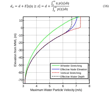
Figure 2. Comparison of water particle kinematics simulated using different methods at 10 m above MWL (Cd = 0.65, Cm = 1.60, Hs = 15m, Tz = 13.75s).

From the aforementioned methods of simulating water particle kinematics, comparison of water particle velocity profile was prepared as illustrated in Figure 2. From the figure, Wheeler stretching is notably at a much lower magnitude than of the other two methods while vertical stretching on the other hand has the highest value of water particle velocity. In the case of effective methods, it lies in between of Wheeler and vertical stretching; however, its water particle velocity profile is leaning closer towards vertical stretching, yet begins to differ as it is approaching the MWL and in the near-surface zone. Upon a closer look, water particle velocity simulated using vertical stretching increases rapidly as it approaches the MWL while abruptly becomes constant at MWL and afterward. This situation is referring to the definition of Eq. (8), where water particle

3 4 5 6 7 8

-70 -60 -50 -40 -30 -20 -10 0 10

Comparison of Water Particle Velocity Profiles from 4 Methods

Maximum Water Particle Velocity (m/s)

(7)

kinematics at above MWL is assumed to be the same as the MWL in the case of vertical stretching. Wheeler stretching, on the other hand, shows a gradual increase in water particle velocity profile starting from seabed towards 10m above MWL. In the case of effective node elevation and effective water depth methods, its water particle velocity profile starts to differ from vertical stretching in the near-surface zone where it offers gradual changes in water particle velocity instead of abruptly becoming constant. Water particle velocities predicted from the effective water depth procedure are somewhat smaller than the corresponding values from the effective node procedure. In fact, there are some similarities between the water particle velocity profiles from the effective water depth and the vertical stretching methods in that in both cases, the velocity profile above MWL is almost vertical. Therefore, the main difference between the two methods is that predicted velocities from the effective water depth procedure are somewhat smaller than those from the vertical stretching method in the near-surface zone. The significant differences in the magnitude of water particle kinematics simulated from vertical and Wheeler stretching have been discovered in several previous studies [14, 15, 19, 20]. While vertical stretching is said to overestimate water particle kinematics in the near-surface zone, Wheeler stretching tends to underestimate it.

Evaluation of Offshore Structural Response by Time Simulation Procedure

The evaluation of the offshore structural response values by time simulation procedure is as follows [31, 32]:

i) Identify the appropriate frequency wave spectrum (i.e. Pierson-Moskowitz spectrum) based on the location of the offshore structure.

ii) Generate surface elevation based on the appropriate frequency wave spectrum at an arbitrary reference point for a given period of time using Eq. (7).

iii) Compute the components of water particle kinematics (velocities and accelerations) at each node elevation using the appropriate transfer function and account for the intermittency load at the member of the splash zone. In this study, the Vertical stretching, Wheeler stretching, effective node elevation and effective water methods were used for this purpose.

iv) Compute the Morison load corresponding to its water particle kinematics.

v) Compute the quasi-static response using Equation (17) and Equation (18) from Morison’s nodal loads.

Base Shear, 𝐵𝑆 = ∑[F_i∗ ∆l_i] 𝑁𝐹

𝑖=1

(17)

Overturning Moment, 𝑂𝑇𝑀 = ∑[F_i∗ ∆l_i∗ z_i] 𝑁𝐹

𝑖=1

(18)

where NF is the number of nodal force, 𝐹_𝑖 is Morison’s force per unit length at node i, ∆𝑙_𝑖 is the length of member associated with node i, and 𝑧_𝑖 is the elevation of node i from seabed. In one complete cycle of response records, the maximum value is considered as the extreme response values.

RESULTS AND DISCUSSION

Effect of Current Loading on 100-year Extreme Structural Responses

(8)

water particle kinematics. The comparison was carried out using different current conditions (0m/s, +0.9m/s and -0.9m/s) at the different level of significant wave heights, Hs (5m, 10m, and 15m) values. The analysis was made on a quasi-static structural response calculated using rough cylindrical surface condition where the coefficients of drag and inertia for both surface conditions were based on the standard code of practice [27].

Absence of Current (𝒖̅ =0.0m/s)

In this section, different methods of simulating water particle kinematics are studied without considering the current effect. Results in Table 1 are expressed in terms of a ratio of the 100-year extreme responses magnitude for the ease of discussion. The ratios of extreme responses were compared to Wheeler stretching as recommended by the American Petroleum Institute [27] for offshore practice. Hence, it is reasonable to look into the difference this method had with its counterparts.

Table 1. Ratios of simulated total extreme responses without current (u̅ = +0.0m/s).

Hs = 5m Hs = 10m Hs = 15m

Method BS OTM BS OTM BS OTM

Wheeler stretching 1.000 1.000 1.000 1.000 1.000 1.000 Effective water depth 1.174 1.240 1.278 1.330 1.208 1.259 Effective node elevation 1.175 1.241 1.284 1.338 1.222 1.277 Vertical stretching 1.222 1.311 1.341 1.414 1.259 1.338

(9)

extreme response. It is to be reminded that the magnitude of extreme response is one critical consideration in the design and analysis of offshore structure.

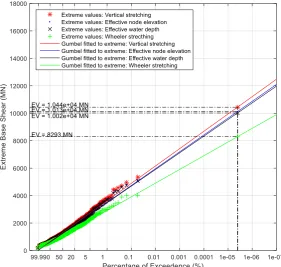
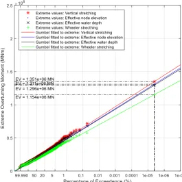
From Figure 3, vertical stretching is found to differ by about 26% from Wheeler stretching; which is equivalent to 2,147MN of difference in magnitude of extreme base shear. On the other hand, both effective methods followed differ by 21% (effective water depth) and 22% (effective node elevation). The same observation can be made in the case of the simulated overturning moment at the same wave height as in Figure 4. However, the difference is much critical with 34% of difference resulted from vertical and Wheeler stretching; which is equivalent to 23,4500 MN.m of difference in magnitude of the extreme overturning moment. Overall, the outputs from Table 1 show vertical stretching was found to differ from the Wheeler stretching method by up to 41% (for the case overturning moment at Hs = 10m). This variation is followed by effective node elevation and effective water depth. The differences are consistent when the 100-year extreme responses are simulated at lower Hs values (e.g., 5m and 10m). From this table, it can be seen that the difference in magnitude of extreme responses at lower Hs values, particularly at 5m, may not be as critical as it was at 10m and 15m of wave heights. However, it is still a primary concern considering the difference in magnitude of extreme responses is too significant and non-negligible. Since the problem is inherent from different methods of simulating water particle kinematics, it would inevitably affect the magnitude of extreme responses to be used in the design and analysis of offshore structure.

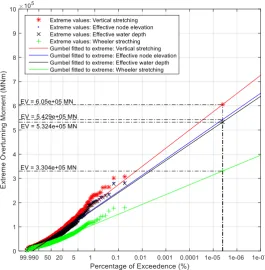
Figure 3. Probability distribution of extreme base shear simulated at Hs=15m, Current=0.00m/s, T=128s & 1000 sample records.

(10)

integral contributor to the total extreme base shear which has 2,147MN of difference in magnitude of extreme base shear as in Figure 3. In contrast, Figure 6 shows that the difference between vertical stretching and Wheeler stretching for the inertial-induced extreme base shear is calculated at only 3.80%; where it is corresponding to only 84MN.m. This shows that the contribution of inertial-induced responses is minimal.

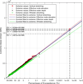
Figure 4. Probability distribution of extreme overturning moment simulated at Hs=15m, Current=0.00m/s, T=128s & 1000 sample records.

(11)

A comparison can be made from both plotted distribution, where it can be clearly seen that drag-induced extreme responses are much more dominant than the inertial-induced extreme responses. This means that drag-inertial-induced extreme response has a greater contribution to the simulated total-extreme extreme responses as in Figure 3 for the case of extreme base shear. This is reasonable and can be reflected by the drag component of the Morison equation, which is proportional to a square of instantaneous wave’s velocity [33]. Inertial element, on the other hand, is in phase with the local wave’s acceleration.

Figure 6: Probability distribution of inertial-induced extreme base shear simulated at Hs=15m, Current=0.00m/s, T=128s & 1000 sample records.

Positive Current (𝒖̅ = +0.9m/s)

(12)

and trailed by its corresponding efficient method; the effective water depth method, by a small variation. From Figure 7, it can be clearly seen that the difference in gap between the probability distributions of extreme base shear is not as much as in the previous current case.

Figure 7. Probability distribution of extreme base shear simulated at Hs=15m, Current=+0.90m.s, T=128s & 1000 sample records.

Table 2. Ratios of simulated total extreme responses with positive current (u̅ = +0.9m/s).

Hs = 5m Hs = 10m Hs = 15m

(13)

Figure 8. Probability distribution of extreme overturning moment simulated at Hs=15m, Current=+0.90m.s, T=128s & 1000 sample records.

Negative Current (𝒖̅ = -0.9m/s)

In the analysis where a negative current loading was considered, the magnitude of -0.9m/s was incorporated. The ratios of the simulated extreme responses are presented in Table 3. This table shows that negative current leads to the lowest magnitude of 100-year extreme responses that its counterparts; the no current and positive current conditions. Further observation of the results shows that although it has a lower magnitude of simulated extreme responses, the results lead to the highest percentage difference. This can be clearly seen as vertical stretching has significantly differed from Wheeler stretching in the range of 26% to 83% difference in magnitude of extreme responses, throughout 5m, 10m and 15m of significant wave heights [34].

Table 3. Ratios of simulated total extreme response with negative current (u̅ = -0.9m/s).

Hs = 5m Hs = 10m Hs = 15m

(14)

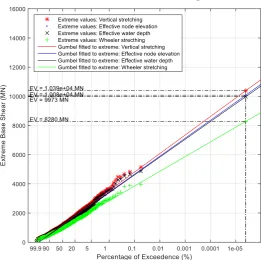
Figure 9. Probability distribution of extreme base shear simulated at Hs=15m, Current=-0.90m.s, T=128s & 1000 sample records.

(15)

There is clearly a huge gap in the probability distribution of extreme base shear between all different methods observed in this current condition. A comparable observation can be made when the analysis is made at lower significant wave heights (Hs = 5m); however, in reference to Table 3, the difference is not as critical as at high significant wave heights (Hs = 15m). As an example, Figure 9 shows that vertical stretching differs from Wheeler stretching by 69%; where it is corresponding to 2,472MN of difference in magnitude of extreme base shear. This is followed by effective water depth and node elevation at 53% and 56% of the variation, respectively. For the simulated extreme overturning moment as in Figure 10, the same remarks can be made, where the difference is a little bit higher for vertical stretching at 83% of the difference from the Wheeler stretching method; this is equivalent to about 274,600MN.m of difference in the magnitude of the extreme overturning moment. Effective water depth and node elevation trailed at 61% and 64% difference, respectively.

CONCLUSIONS

a) LRWT is an often used method to calculate water particle kinematics; although it is able to predict sensible kinematics at points below MWL, it may not be the case for prediction at the near-surface or points above the MWL. The problem is the rapid growth of water particle kinematics, particularly for high-frequency wave component.

b) Empirical methods have been introduced as the means to provide a better representation of water particle kinematics in the near-surface. Some of the most often used methods are such as Wheeler stretching, vertical stretching, delta stretching and linear extrapolation methods. Although these methods are introduced to predict more sensible kinematics at points above MWL, yet their respective results differ significantly, one from another.

c) Examination of the ratios in Table 1 (without current), Table 2 (positive current) and Table3 (negative current) indicates that in all cases, the vertical method has the highest ratios and that the ratios for effective node elevation and effective water depth methods are between those from Wheeler and vertical stretching methods.

d) As observed, for all current cases, the highest vertical ratios for zero, positive and negative current cases are 1.414, 1.175 and 1.831, respectively. It is observed that even for positive-current cases, the difference between Wheeler and vertical stretching predictions is quite high and cannot be neglected. Same ratios from the effective water depth procedure are 1.33, 1.138 and 1.611, respectively. In view of the general belief that the vertical stretching method can over-predict the responses, the effective water depth procedure seems to be more suitable for practical application.

e) It is also observed that the ratios are closer to unity for the positive current cases. This is because current is the same for both Wheeler and vertical stretching methods. Since the current is positive, a certain fixed amount will be added to wave-induced horizontal water particle velocities and hence the ratio between water particle velocity (current + wave-induced) from Wheeler to that from vertical stretching will be closer to unity as a result of the addition of the current. f) The opposite effect explains why in the case of negative current, the ratios have

(16)

100-year predictions from the Wheeler and the vertical stretching methods are too large to be neglected and therefore, further investigation is necessary to resolve this problem. In the meantime, the use of effective water depth procedure is recommended.

g) For all current conditions, the difference in magnitude of extreme responses when simulated using various methods of simulating water particle kinematics is relatively substantial and should not be neglected. Vertical stretching is found to differ significantly from Wheeler stretching, although these methods are the most often used methods in offshore practice. American Petroleum Institute [27][27] recommends Wheeler stretching, while vertical stretching is desirable due to its efficiency. Efficient methods, on the other hand, offer an alternative as they lie in between the vertical and Wheeler stretching. These methods offer a better option for better estimation of water particle kinematics and efficiency in computation. h) In this study, the investigation was carried out based on short simulated records

(128 seconds). However, it is commonly assumed that a sea state lasts for a few hours (say 3 hours). This does not cause any problem as the probability distribution of the extreme values during a 3 hour period can be obtained by assuming that the extreme values of successive short segments (128 seconds) are statistically independent from each other.

i) It would be desirable to extend this study to investigate the effects on the long-term probability distribution of extreme responses as a much accurate 100-year extreme response can be produced in comparison to the short-term probability distribution of extreme responses, which was used in this study as a preliminary study. Furthermore, the results of this study can be compared with a high-quality laboratory and field data in order to obtain their accuracy when compared to measured data. Other than that, they could also be compared to more accurate nonlinear models such as the Hybrid Wave Model (HWM).

ACKNOWLEDGEMENTS

This paper is ﬁnancially supported by the Universiti Teknologi Malaysia (UTM), [grant number Q.K130000.2540.18H09 and Q.K130000.2540.17H99] which is gratefully acknowledged.

REFERENCES

[1] Najafian G. Local hydrodynamic force coefficients from field data and probabilistic analysis of offshore structures exposed to random wave loading: University of Liverpool, Liverpool; 1991.

[2] Mellor G. A combined derivation of the integrated and vertically resolved, coupled wave–current equations. Journal of Physical Oceanography. 2015;45:1453-63.

[3] Kim DK, Zalaya MA, Mohd MH, Choi HS, Park KS. Safety assessment of corroded jacket platform considering decommissioning event. International Journal of Automotive and Mechanical Engineering. 2017;14:4462-85.

(17)

[5] Morison J, Johnson J, Schaaf S. The force exerted by surface waves on piles. Journal of Petroleum Technology. 1950;2:149-54.

[6] Smit P, Janssen T, Herbers T. Nonlinear Wave Kinematics near the Ocean Surface. Journal of Physical Oceanography. 2017;47:1657-73.

[7] Haver SK, Edvardsen K, Lian G. Uncertainties in wave loads on slender pile structures due to uncertainties in modelling waves and associated kinematics. The 27th International Ocean and Polar Engineering Conference: International Society of Offshore and Polar Engineers; 2017.

[8] Abu Husain MK, Mohd Zaki NI, Najafian G. Derivation of the probability distribution of the extreme values of offshore structural response by an efficient time simulation method. The Open Civil Engineering Journal. 2013;7:61-272. [9] Chalikov D, Babanin AV, Sanina E. Numerical modeling of 3D fully nonlinear

potential periodic waves. Ocean dynamics. 2014;64:1469-86.

[10] Melville WK, Fedorov AV. The equilibrium dynamics and statistics of gravity– capillary waves. Journal of Fluid Mechanics. 2015;767:449-66.

[11] Wheeler J. Methods for calculating forces produced by irregular waves. Offshore Technology Conference: Offshore Technology Conference; 1969.

[12] Marshall P, Inglis R. Wave kinematics and force coefficients. ASCE structures congress1986. p. 15-8.

[13] Rodenbusch G, Forristall G. An empirical model for random directional wave kinematics near the free surface. Offshore Technology Conference: Offshore Technology Conference; 1986.

[14] Couch A, Conte J. Field verification of linear and nonlinear hybrid wave models for offshore tower response prediction. Journal of Offshore Mechanics and Arctic Engineering. 1997;119:158-65.

[15] Zhang J, Chen L, Ye M, Randall RE. Hybrid wave model for unidirectional irregular waves—part I. Theory and numerical scheme. Applied Ocean Research. 1996;18:77-92.

[16] Rascle N, Chapron B, Ponte A, Ardhuin F, Klein P. Surface roughness imaging of currents shows divergence and strain in the wind direction. Journal of Physical Oceanography. 2014;44:2153-63.

[17] Spell C, Zhang J, Randall RE. Hybrid wave model for unidirectional irregular waves—part II. Comparison with laboratory measurements. Applied Ocean Research. 1996;18:93-110.

[18] Longridge J, Randall R, Zhang J. Comparison of experimental irregular water wave elevation and kinematic data with new hybrid wave model predictions. Ocean Engineering. 1996;23:277-307.

[19] Najafian G, Zaki NM, Aqel G. Simulation of water particle kinematics in the near surface zone. ASME 28th International Conference on Ocean, Offshore and Arctic Engineering: American Society of Mechanical Engineers; 2009. p. 157-62. [20] Zaki NM, Najafian G. Derivation of water particle kinematics in the near surface zone by the effective water depth procedure. ASME 2010 29th International Conference on Ocean, Offshore and Arctic Engineering: American Society of Mechanical Engineers; 2010. p. 295-300.

(18)

[22] Pizzo N, Deike L, Melville WK. Current generation by deep-water breaking waves. Journal of Fluid Mechanics. 2016;803:275-91.

[23] Pizzo N, Melville WK. Wave modulation: the geometry, kinematics, and dynamics of surface-wave packets. Journal of Fluid Mechanics. 2016;803:292-312.

[24] Sarpkaya T, Isaacson M. Mechanics of wave forces on offshore structures. 1981. [25] Fujimoto W, Waseda T. Nonlinear Effects on Local Mechanics of Freak Waves.

ASME 34th International Conference on Ocean, Offshore and Arctic Engineering: American Society of Mechanical Engineers; 2015. p. V007T06A83-VT06A83. [26] Mirzadeh J, Kimiaei M, Cassidy MJ. Performance of an example jack-up platform

under directional random ocean waves. Applied Ocean Research. 2016;54:87-100.

[27] (API) API. Recommended practice for planning, designing and constructing fixed offshore platforms — Working stress design (22nd Edition). 2014.

[28] Kajishima T, Takeuchi S. Simulation of fluid-structure interaction based on an immersed-solid method. Journal of Mechanical Engineering and Sciences. 2013;5:555-61.

[29] Pierson WJ, Moskowitz L. A proposed spectral form for fully developed wind seas based on the similarity theory of SA Kitaigorodskii. Journal of geophysical research. 1964;69:5181-90.

[30] Mohd Zaki N, Abu Husain M, Najafian G. Extreme structural response values from various methods of simulating wave kinematics. Ships and Offshore Structures. 2016;11:369-84.

[31] Deo M. Waves and Structures. Mumbai: Indian Institute of Technology Bombay. 2013.

[32] Mukhlas NA, Shuhaimy NA, Johari MB, Soom EM, Khairi M, Husain A, et al. Design and analysis of fixed offshore structure–an overview. Malaysian Journal of Civil Engineering. 28(3): 503–520

[33] Zaki NM, Husain MA, Wang Y, Najafian G. Short-Term Distribution of the Extreme Values of Offshore Structural Response by Modified Finite-Memory Nonlinear System Modeling. ASME 32nd International Conference on Ocean, Offshore and Arctic Engineering: American Society of Mechanical Engineers; 2013. p. V02ATA049-V02AT02A.