Study of Rayleigh Taylor Instability with the help of CFD simulation
Indrashis SahaDepartment of Chemical Engineering, University of Calcutta, Kolkata, India; Email: [email protected]
ABSTRACT: The purpose of this paper is to simulate a two-dimensional Rayleigh-Taylor instability problem using the classical method of Finite Element analysis of a multiphase model using ANSYS FLUENT 19.2. The governing equations consist of a system of coupled nonlinear partial differential equations for conservation of mass, momentum
and phase transport equations. The study focuses on the transient state simulation of Rayleigh Taylor waves and subsequent turbulent mixing in the two phases incorporated in the model. The Rayleigh Taylor instability is an
instability of an interface between two fluids of different densities which occurs when the lighter fluid is pushing the heavier fluid in a gravitational field. The problem was governed by the Navier-Stokes and Cahn-Hilliard equations in
a primitive variable formulation. The Cahn- Hilliard equations were used to capture the interface between two fluids systems. The objective of this article is to perform grid dependency test on Rayleigh Taylor Instability for 2 different
mesh size and compare the results for the variation in Atwood Number. The results were validated with the observations from previous published literatures.
Keywords:CFD Simulation, Transient state, Rayleigh Taylor Instability, Multiphase Flow
Introduction
In Multiphase flow, the dynamic variables like the velocity, viscosity, pressure and density are generally used to
explain the movement of fluids under the gravitational field. Multiphase flows takes place in nuclear geothermal power
plants, food processing industries and many others. One of the basic example is Rayleigh Taylor Instability. The Rayleigh Taylor Instability is a hydrodynamic instability arises when a high density fluid is placed over a low density
fluid in a gravitational field. The RTI phenomenon was initially introduced by Rayleigh 1883 and later was observed for all accelerated fluids by Taylor 1950. When the density interface is disturbed, the hydrostatic pressure is generated, so the heavier fluid moves downwards and mixes with the lighter one, with the amplitude of perturbation initially growing exponentially but after sometime saturates and forms characteristic mushroom shape. When a heavier fluid
is displaced downward with an equal volume of lighter fluid displaced upwards, it results in decrease of potential energy than it’s initial state. This RTI has been applied to a wide range of problems including the mushroom clouds
like volcanic eruptions, nuclear explosions and plasma fusion reactors instability.
Presently large number of numerical techniques were introduced to simulate RTI including boundary integral methods( Baker et al. 1984), front tracking methods( Liu et al. 2007, Terashima and Tryggvason 2009), volume of fluid methods(Hirt and Nichols 1981, Gopala and BGMvan 2008,Raessi et al. 2010) and phase field methods(Ding et al. 2007, Chiu and Lin 2011, Lee et al. 2011, Kim 2005). Cheng et al. 2012 numerically simulated RTI by using a moving particle semi-implicit method that was well validated with experimental results. Discontinuous Galerkin method was used to simulate the multi-layered Richtmyer-Meshkov and RTI problems(Henry de Frahen et al. 2015). Tryggvason 1988 used Lagrangian-Eulerian vortex methods for simulating the dynamics of perturbation in two fluid model. Zhang 1991 conducted numerical investigation to study the motion of spikes in RT interfaces by applying front tracking method on 2D Euler equations. Talat et al.2018 introduced the diffuse approximated method(DAM) and phase field formulation for solving 2D RTI problem where the fluids were assumed as incompressible and immiscible. Lee et al. 2011 used a phase field method with periodic boundary conditions to simulate the dynamics of RT interface which was based on coupled solving of both Navier Stokes equation and Cahn-Hilliard equation in the terms of all the primitive parameters or variables in the 2D staggered grid .Gou et al. 2018 used the multiphase moving
particle semi-implicit(MMPS) with periodic boundary conditions to simulate RTI of the immiscible two phase incompressible fluid. The effect of initial perturbation wavelength, surface tension and Atwood Number was
investigated in the single mode RTI problem and it was observed that the numerical results were in good agreement with the analytical results.
A numerical study on the dynamics of spherical bubble rising in quiescent liquid with finite volume method, was
performed by Tripathi et al. 2015. Further on, numerous experimental and numerical investigation on rising bubble dynamics was reported by ( Oshagi et al. 2019, Liu et al. 2015, Xu et al. 2017, Cubeddu et al. 2017). Due to numerous experimental studies conducted by (Read 1984, Marinak et al. 1998) it is understood that RTI is a spatial process. Due to the complexity of the implications of 3D simulations, 2D simulations are studied extensively in recent years.
Zhou et al. 2018 implemented 2D Large Eddy Simulation(LES) for investigating the dynamics and the evolution of Rayleigh Taylor bubbles from W-shaped, sinusoidal and random perturbations. The classical numerical methods such
as the Finite Difference method, Finite Volume method, Finite Element method has been extensively used to solve
physical problems in science and engineering but the implementation of these classical methods has certain drawbacks. The main drawback is that these classical methods is required to build a mesh in the computational domain and on the
boundaries to solve the problem.
However the present study is based on the Finite Element method to simulate the interface evolution of RTI. Here in
this study the 2D geometry is itself constructed in Spaceclaim and a computational mesh is generated. The meshing
file is imported in fluent and a grid dependency test was performed and the results of the interfacial evolution of RTI is captured at different flow times and compared. The governing equations for the RTI were the modified form of both
Navier-Stokes equation and Cahn-Hilliard equation. The spatial discretization involves least square cell based for gradient and for time derivative, first order implicit scheme was used in order to solve the governing equations.
SIMPLE scheme was employed to overcome the pressure velocity coupling. In this study the density of the secondary phase is altered with the incorporation of user defined material resulting in variation of Atwood Number. The results
of the grid dependency study and the variation of Atwood Numbers are carefully observed and reported in the present literature.
Governing Equations
The governing equations for The RTI problem are the Navier–Stokes equations, the continuity and the Cahn-Hilliard equations which are the non-dimensional form.
𝜕𝑢 𝜕𝑡 + 𝑢 𝜕𝑢 𝜕𝑥+ 𝑣 𝜕𝑢 𝜕𝑦= − 1 𝜌(𝑐) 𝜕𝑝 𝜕𝑥+ 1 𝑅𝑒 ∙ 𝜌(𝑐)(
𝜕2𝑢 𝜕𝑥2+
𝜕2𝑢 𝜕𝑦2) 𝜕𝑣 𝜕𝑡 + 𝑢 𝜕𝑣 𝜕𝑥+ 𝑣 𝜕𝑣 𝜕𝑦= 1 𝜌(𝑐) 𝜕𝑝 𝜕𝑦+ 1 𝑅𝑒 ∙ 𝜌(𝑐)(
𝜕2𝑣 𝜕𝑥2+
𝜕2𝑣 𝜕2𝑦) +
𝑔 𝐹𝑟
𝜕𝑢 𝜕𝑥+
𝜕𝑣 𝜕𝑦= 0
𝜕𝐶 𝜕𝑡 + 𝑢 𝜕𝑐 𝜕𝑥+ 𝑣 𝜕𝑐 𝜕𝑦= 1 𝑃𝑒(
𝜕2𝜇 𝜕𝑥2+
𝜕2𝜇 𝜕𝑦2)
𝜇 = 𝑐3− 𝐶ℎ2( 𝜕2𝑐 𝜕𝑥2+
The above equations can be reduced into non-dimensionalized form as follows
𝑥
′=
𝑥 𝐿𝑐,
𝑢
′=
𝑢 𝑈𝑐,
𝑡
′=
𝑡𝑈𝑐 𝐿𝑐,
𝜌
′=
𝜌 𝜌𝑐,
𝑝
′=
𝑝𝜌𝑐𝑈𝑐2
,
𝜂
′
=
𝜂 𝜂𝑐,
𝑔
′=
𝑔 𝑔𝑐,
𝜇
′=
𝜇 𝜇𝑐where ‘ represents non-dimensional values. The Reynolds number ( Re ), Peclet number ( Pe ), Cahn number ( Ch ) and Froude number ( Fr ) are defined as
𝑅𝑒 =
𝜌𝑐𝑈𝑐𝐿𝑐𝜂𝑐
,
𝑃𝑒 =
𝑈𝑐𝐿𝑐
𝑀𝜇
,
𝐶
ℎ= √
𝜖𝛼𝐿𝑐2
,
𝐹𝑟 =
𝑈𝑐
√𝑔𝐿𝑐
The periodic boundary conditions are used on the left and right boundaries ( x = 0 and x = L ), and 𝑢 = 𝑣 =𝜕𝑝 𝜕𝑦=
𝜕𝑐 𝜕𝑦= 𝜕𝜇
𝜕𝑦= 0 , 𝜕𝑝 𝜕𝑦= −
𝜌
𝐹𝑟. Following this the pressure velocity is coupled to solve the momentum equation. Here the
intermediate values does not satisfy the mass continuity equation for which the intermediate velocities are corrected by pressure terms. After finishing with the calculation of u, v and p, concentration, c and chemical potential μ and Cahn-Hilliard equations are solved by semi implicit scheme which is followed by spatial discretization of momentum
equation by second order upwind and pressure by PRESTO.
Preprocessing and Mesh
At first, geometry is created as square boxes and converted to surface using Pull tool and share topology is turned
on.The geometry was created in spaceclaim and it involves no other importing of CAD models. The surface model
was further processed for meshing and the results were taken for three different meshing schemes. This preprocessing phase of the workflow is extremely important because it determines the simulation potential and limits the CFD results.
• Case A. Mesh details: Baseline mesh- 0.5mm Element size, Elements – 3200, Nodes – 332
• Case B. Mesh details: Mesh - 0.18mm Element size, Elements – 24642, Nodes – 24976
• Case C. Mesh details: Mesh - 0.1 mm Element size, Elements – 80000, Nodes – 80601
CFD Case Setup
• Pressure based solver and Absolute velocity is used.
• Transient-state Calculation is performed.
• Compressible fluid flow is chosen.
• Gravity is enabled in -ve Y axis
• Multiphase Model is turned on along with Volume of Fluid and number of Eulerian phases is chosen as 2 and Implicit scheme is selected.
• Viscous model-Laminar is used.
• Cell zone selected as Fluid-air;water-surface:water-liquid
• Patching of the volume fraction of the two phases is performed before the start of simulation.Phase used for patching was water and volume fraction of 1 is taken for water surface and 0 for air surface.
Post-processing Results
The post processing was done in CFD Fluent. Case 1 is for the meshing scheme and Case 2 is for the variation in Atwood Number
For Case 1A: The transient case was run for 2000 time steps with a Time step size of 0.005. A more clearer settled fluids are observed. We can observe from the water volume fraction how the air has moved upwards while the water settles down. For Case 1B: This case was ran for 4000 time steps with a time step size of 0.0005. As the mesh size is increased we get more defined results which we can see from the below plot and it took a long time for the simulation to reach appropriate results.
Case 2A, 2B, 2C: This case was ran for 2000 time steps with a time step size of 0.005 with the meshing that of Case 1A.The change is that the density of the secondary phase is varied with the inclusion of user defined material to make Artwood Number to 0.3, 0.4 and 0.5 for 2A,2B and 2C respectively.
In the following section, we analyzed the R-T instability phenomena for two immiscible incompressible fluids having different densities (Primary phase, 𝜌1= 1.225 𝑘𝑔/𝑚3 and Secondary phase, 𝜌2= 998.2𝑘𝑔/𝑚3 ) with different viscosities(𝜇1= 0.17894,𝜇2= 0.001003). For a planar interface at the equilibrium, the concentration interface is given by the hyperbolic tangent function as suggested by Lee et al. 2013 as follows:
𝜙(𝑥, 𝑦, 0) = tanh (𝑦 − 2 − 0.1 cos(2𝜋𝑥)
√2𝐶ℎ )
The initial interface profile is perturbed by cosine wave of amplitude 0.1. The numerical parameters are ∆𝑡 =
0.005,𝐶ℎ = 0.01, 𝑅𝑒 = 3000,𝐴𝑡 = 0.998 and 𝑃𝑒 = 1
𝐶ℎ . In this study the governing equations are solved by implicit scheme, henceforth the transient simulation is unconditionally stable. There is no limitation for the time step size to ensure stability however time step size of 0.005 was taken. The Chan Number(Ch) is the ratio of interface thickness to the width of the domain. In this study 𝐶ℎ = 0.01 is chosen as that chosen by Lee et al. 2013 and Katavkar 2005..At higher Reynolds Number the viscous effect is negligible. Budiana et al. 2020 in their study observed that the evolution of the interface grows faster with the increase in Atwood Number for which in this study the Atwood Number is kept as high as possible in Case 1A. It was seen that with larger Atwood Number, larger amplitude of perturbations are observed. It is due to the larger density ratio of the two fluids, the stronger is the force to develop the interface instability.The Atwood Number is a dimensionless number in Fluid Dynamics. It is used in the study of instabilities of the dynamics of the fluid flow.It gives the relation between density of higher fluid and the density of lighter fluid. For Atwood no. close to 0, RT instability flows takes the form of symmetric "fingers" of fluid.
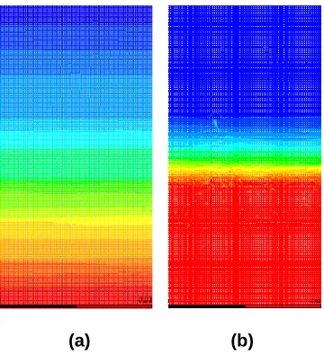
(a) (b)
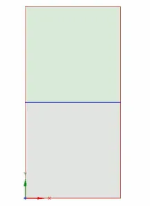
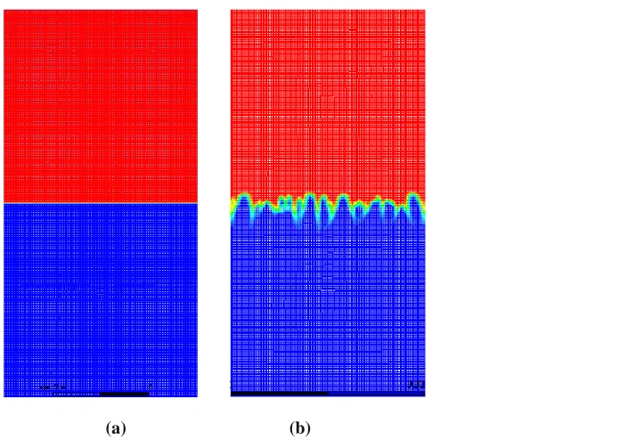
Figure 2:. The initial perturbation is given by 𝝓(𝒙, 𝒚, 𝟎) = 𝐭𝐚𝐧𝐡 (𝒚−𝟐−𝟎.𝟏 𝐜𝐨𝐬(𝟐𝝅𝒙)
√𝟐𝑪𝒉 )in figure 1(a) at 𝒕 = 𝟎
and its simulation at time t = 0.025 in figure 1(b).
Plots on Water Volume Fraction
(a) (b) (c) (d) (e)
(f) (g) (h) (i) (j)
(k) (l) (m) (n) (o)
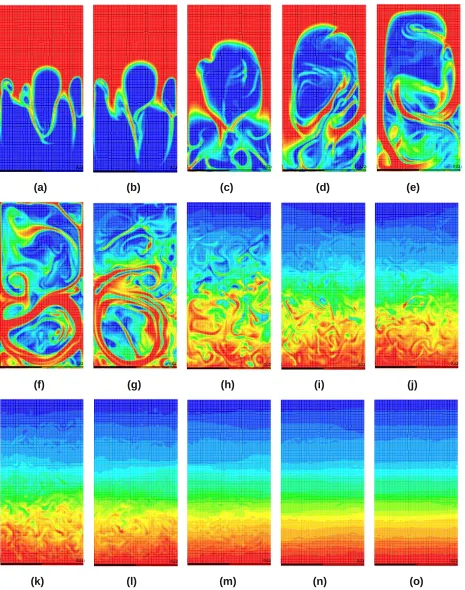
Figure 3: Penetration of heavier fluid into lighter one for Case A at different flow times (a)0.0945s, (b)0.11s, (c)0.15s, (d)0.195s, (e)0.25s, (f)0.35s, (g)0.515s, (h)0.92s, (i)1.23s, (j)1.415s, (k)1.535s,
(a) (b) (c) (d) (e)
(f) (g) (h) (i) (j)
(k) (l) (m) (n) (o)
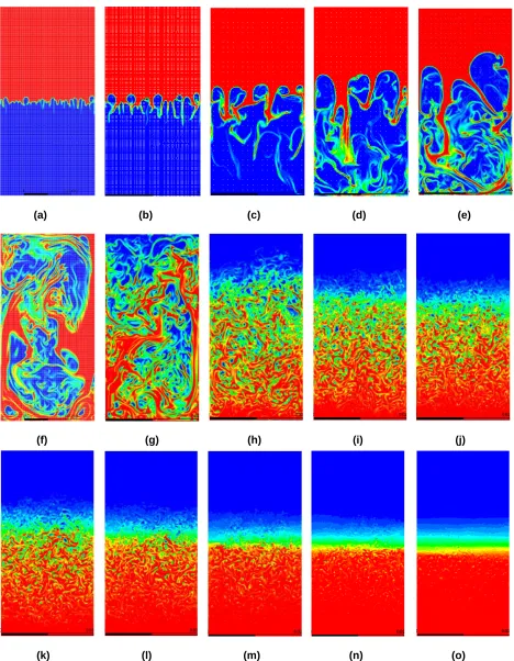
Figure 4: Penetration of heavier fluid into lighter one for Case B at different flow times (a)0.0945s, (b)0.11s, (c)0.1495s, (d)0.198s, (e)0.242s, (f)0.349s, (g)0.519s, (h)0.918s, (i)1.23s, (j)1.4105s,
(a) (b)
Figure 5: Interface in the verge of Complete Settling;(a) Case A at Flow time 7.7s,(b) Case B at Flow time 7 s
Comparison of Variation in Atwood Number with Case 1A
With the decrease in Atwood Number from Case 1A and 1B from 0.9 to 0.3,0.4 and 0.5 for 2A, 2B and 2C respectively and when compared, we can clearly observe from Figure 7 and 8 that bubbles and spikes formation are still present at
the same flow time or even after completion of simulation or at the verge of settling.The formation is because of the
increase in density of secondary phase with a density of (𝜌2𝐴= 536.846 𝑘𝑔
𝑚3 , 𝜌2𝐵 = 427.285 𝑘𝑔
𝑚3 , 𝜌2𝐶 = 332.33 𝑘𝑔 𝑚3)
for Case 2A, 2B and 2C respectively. For the case of smaller Atwood Number, the density difference between the two
sides of the interface is small and the density distribution of the upper and lower layers is nearly symmetrical. The initial density stratification plays a dominant role and the expansion compression effect has a little influence. With the
increased Atwood Number close to 1 the stabilization effect of initial density stratification decreases and the instability caused by the expansion-compression effect becomes more significant. It can be seen in the figures that the larger Atwood numbers, the larger amplitude ofperturbation. It takes place due to the larger density ratio of two fluids is, the
stronger force to develop the interface instability. The flow structure of bubbles and globules are quite different both for the variation in meshing and also with the variation in Atwood Number. The increase of Atwood number, the time
of spikes or globules of the lighter phase fluid arriving at the bottom of the computational domain is accelerated, then the duration of RTI in the steady growth stage is shorter. We can observe that the compressibility on the bubble
velocity is strong at larger Atwood Number. The bubble height is approximately a quadratic function of time at potential flow growth stage. The average bubble acceleration is nearly proportional to the square of the Mach Number
of Atwood Number close to 1.For Atwood No. close to 1, the much lighter fluid below the heavier fluid takes the
form of larger bubble like plumes.Since in our simulation for Case 1A and 1B has Atwood Number close to 1, heavier fluid takes bubble form and thus helping in validating that our simulation is correct.
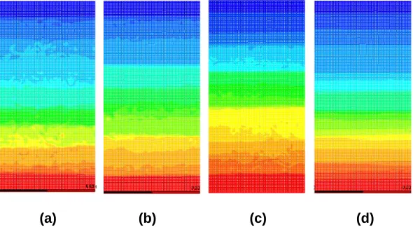
(a) (b) (c) (d)
Figure 6: Penetration of heavier fluid into lighter one at flow time 0.515 s; (a)At=0.3(Case 2A) (b)At=0.4(Case 2B) (c)At=0.5(Case 2C) (d) At=0.9(Case 1A)
(a) (b) (c) (d)
Figure 7:Contour showing Volume Fraction of secondary phase at intermediate flow time of 3.6 s; (a)At=0.3(Case 2A) (b)At=0.4(Case 2B) (c)At=0.5(Case 2C) (d) At=0.9(Case 1A)
(a) (b) (c) (d)
Conclusions
In the present manuscript, classical method of Finite Element analysis was adopted to study the evolution of the interface during RTI. The governing equations were Navier-Stokes equations and Cahn-Hilliard equations. The initial
displacement disturbance was defined by the Cosine function. Steady state solution determines the fully developed solution. This numerical simulation was validated with the observations obtained by previous researchers and this was
done by the variation in Atwood Number where we obtained the same observation. In lower Atwood numbers, spikes and globules were still present at the end of the simulation which was not there in Atwood Number of 0.9 in Case 1A.
From the grid dependency we also observed that the interface thickness reduces with the refined mesh and when run
with smaller time steps.For Transient simulation, compared to steady state, has higher demand in terms of computational time. Transient solver better captures the flow and can be used to run at smaller time steps which is
seen from the Case 1B with a time step size of 0.0005. Smaller time steps are required to observe the instabilities and can be only possible through transient simulation. Since it is a time marching solution, we expect more accuracy from
transient simulation for which Transient simuation is the ideal setup to run the calculation for Rayleigh Taylor Instability.
References
Baker, G. R., Meiron, D. I., & Orszag, S. A. (1984). Boundary integral methods for axisymmetric and three-dimensional Rayleigh-Taylor instability problems. Physica D: Nonlinear Phenomena, 12(1-3), 19-31.
Budiana, E. P. (2020). Meshless numerical model based on radial basis function (RBF) method to simulate the Rayleigh–Taylor instability (RTI). Computers & Fluids, 201, 104472.
Cheng, H., Jiang, S., Bo, H., & Duan, R. (2012). Numerical simulation of the Rayleigh-Taylor instability using the MPS method. Science China Technological Sciences, 55(10), 2953-2959.
Chiu, P. H., & Lin, Y. T. (2011). A conservative phase field method for solving incompressible two-phase
flows. Journal of Computational Physics, 230(1), 185-204.
Cubeddu, A. , Rauh, C. , Ulrich, V. , (2017). Simulations of bubble growth and interaction in high viscous fluids using
the lattice Boltzmann method. Int. J. Multip. Flow 93, 108–114 .
de Frahan, M. H., Movahed, P., & Johnsen, E. (2015). Numerical simulations of a shock interacting with successive
interfaces using the Discontinuous Galerkin method: the multilayered Richtmyer–Meshkov and Rayleigh–Taylor instabilities. Shock Waves, 25(4), 329-345.
Ding, H., Spelt, P. D., & Shu, C. (2007). Diffuse interface model for incompressible two-phase flows with large
density ratios. Journal of Computational Physics, 226(2), 2078-2095.
Gopala, V. R., & van Wachem, B. G. (2008). Volume of fluid methods for immiscible-fluid and free-surface
flows. Chemical Engineering Journal, 141(1-3), 204-221.
Guo, K., Chen, R., Li, Y., Tian, W., Su, G., & Qiu, S. (2018). Numerical simulation of Rayleigh-Taylor Instability
with periodic boundary condition using MPS method. Progress in Nuclear Energy, 109, 130-144.
Kim, J. (2005). A diffuse-interface model for axisymmetric immiscible two-phase flow. Applied mathematics and computation, 160(2), 589-606.
Khatavkar, V. V. (2005). Capillary and low-inertia spreading of a microdroplet on a solid surface.
Lee, H. G., Kim, K., & Kim, J. (2011). On the long time simulation of the Rayleigh–Taylor instability. International journal for numerical methods in engineering, 85(13), 1633-1647.
Liu, X., Li, Y., Glimm, J., & Li, X. L. (2007). A front tracking algorithm for limited mass diffusion. Journal of Computational Physics, 222(2), 644-653.
Lord, R. (1900). Investigation of the character of the equilibrium of an incompressible heavy fluid of variable density. Scientific papers, 200-207.
Liu, L. , Yan, H. , Zhao, G. , (2015). Experimental studies on the shape and motion of air bubbles in viscous liquids. Exp. Ther. Fluid Sci. 62, 109–121 .
Marinak, M.M. , Glendinning, S.G. , Wallace, R.J. , Remington, B.A. , Budil, K.S. , Haan, S.W. , Kilkenny, J.D. ,
(1998). Nonlinear Rayleigh-Taylor evolution of a three- -dimensional multimode perturbation. Phys. Rev. Lett. 80 (20), 4426 .
Oshaghi, M.R. , Shahsavari, M. , Afshin, H. , Firoozabadi, B. , (2019). Experimental inves- tigation of the bubble motion and its ascension in a quiescent viscous liquid. Exp. Ther. Fluid Sci. 103, 274–285 .
Raessi, M., Mostaghimi, J., & Bussmann, M. (2010). A volume-of-fluid interfacial flow solver with advected
normals. Computers & Fluids, 39(8), 1401-1410.
Read, K.I. , (1984). Experimental investigation of turbulent mixing by Rayleigh-Taylor instability. Physica D
Nonlinear Phenomena 12, 45–58 .
Talat, N., Mavrič, B., Hatić, V., Bajt, S., & Šarler, B. (2018). Phase field simulation of Rayleigh–Taylor instability with a meshless method. Engineering Analysis with Boundary Elements, 87, 78-89.
Taylor, G. I. (1950). The instability of liquid surfaces when accelerated in a direction perpendicular to their planes.
I. Proceedings of the Royal Society of London. Series A. Mathematical and Physical Sciences, 201(1065), 192-196. Terashima, H., & Tryggvason, G. (2009). A front-tracking/ghost-fluid method for fluid interfaces in compressible
flows. Journal of Computational Physics, 228(1
Tryggvason, G. , (1988). Numerical simulations of the Rayleigh-Taylor instability. J. Comput. Phys. 75 (2), 253–282
Tripathi, M.K. , Sahu, K.C. , Govindarajan, R. , (2015). Dynamics of an initially spherical bubble rising in quiescent
liquid. Nat. Commun. 6, 6268 .
Xu, X. , Zhang, J. , Liu, F. , Wang, X. , Wei, W. , Liu, Z. , (2017). Rising behavior of sin- gle bubble in infinite
stagnant non-Newtonian liquids. Int. J. Multip. Flow 95, 84–90 .
Zhang, Q. , (1991). The motion of a single bubble or spike in Rayleigh-Taylor unstable interfaces. IMPACT of
Comput. Sci. Eng. 3 (4), 277–304 .
Zhou, Z.R. , Zhang, Y.S. , Tian, B.L. , (2018). Dynamic evolution of Rayleigh-Taylor bub- bles from sinusoidal,