High Resolution Boiling Simulation Using Interface Tracking Method.

(1)

LI, MENGNAN. High Resolution Boiling Simulation Using Interface Tracking Method. (Under the direction of Dr. Igor A. Bolotnov).

Boiling, as one of the most efficient heat transfer mechanisms, is widely used in various

engineering systems. Better understanding and modeling of this process remains a major challenge

in multiphase flow research. In light water reactor (LWR) nuclear power plants, the distribution of

vapor in the reactor core sub-channels affects the heat transfer rate and may cause unfavorable

conditions, such as departure from nucleate boiling (DNB) phenomenon. DNB, in turn, may cause

fuel cladding damage, which may lead to reactor unplanned shutdowns and even accidents. The

advances in High-Performance Computing (HPC) in recent years make it possible to apply direct numerical simulation (DNS) approach to a wide variety of bubble hydrodynamics and

thermodynamics studies. After the interface tracking methods (ITM) are introduced to DNS, the

instantaneous velocity and temperature field at, and around, the interface can be calculated in

two-phase flow simulations. ITM approach provides not only detailed physical description associated

with thermal and hydrodynamic processes but also the shape of the evolving interface, which may

provide new insight on the understanding of boiling phenomenon and help the model development

for multiphase computational fluid dynamics (M-CFD) in the near future.

The high resolution boiling simulations in the presented research are conducted in full

three-dimensional (3D) transient representation with the unstructured grid. This approach allows

us to investigate the boiling phenomenon in various conditions with lower computational cost (by

utilizing local mesh refinement for bubble growth region). To represent more accurate contact

angle during nucleate boiling, the contact angle force model developed in the research group has

been coupled with the evaporation and condensation algorithm. The Bubble Tracking Algorithm

(2)

level-simulations and collect heat transfer information of interest (e.g. evaporation heat flux, bubble

departure diameter, etc.) under various boiling conditions.

The verification of the evaporation and condensation model has been performed by

comparing the bubble growth rate with analytical solutions. Both pool boiling and flow boiling

simulations are performed with the ITM boiling model in PHASTA. The simulated bubble

nucleation frequency in pool boiling simulation is validated against experimentally-based

correlations. The bubble evolution and growth rate is compared with experimental data to validate

the model performance under flow boiling condition. The multi-bubble flow boiling simulation

explores the potential of current model in solving boiling problems with complex geometries.

The presented research lays the foundation of high resolution boiling simulation in

PHASTA. To the author’s best knowledge, it’s the first time that an ITM-based boiling model can

conduct boiling simulations with 3D unstructured mesh. Compared to the structured grid-based

solvers which are challenging to apply to complex engineering geometries, this boiling model

implementation is capable of conducting high resolution large scale boiling simulations in

engineering geometries and resolves the detailed hydrodynamics and thermodynamics information

for quantities of interest at/around the interface. It can help fulfill the numerical data gap between

(3)

(4)

by Mengnan Li

A dissertation submitted to the Graduate Faculty of North Carolina State University

in partial fulfillment of the requirements for the degree of

Doctor of Philosophy

Nuclear Engineering

Raleigh, North Carolina 2019

APPROVED BY:

_____________________________ _____________________________ Dr. Igor A. Bolotnov Dr. Nam T. Dinh

Committee Chair

_____________________________ _____________________________ Dr. J. Michael Doster Dr. Hong Luo

(5)

ii

DEDICATION

(6)

iii

BIOGRAPHY

The author graduated from Sichuan University, China with a bachelor’s degree in Nuclear

Engineering in 2014. She joined the nuclear engineering department of North Carolina State

University in 2014 and started to work with Dr. Igor Bolotnov. She obtained her master’s degree

in 2016. Her research focuses on the ITM boiling model development and high resolution boiling

(7)

iv

ACKNOWLEDGEMENTS

First, I would like to thank Dr. Igor Bolotnov for guiding my research in the past four and

half years. It is a greatest honor for me to be his student. His talent, knowledge and great passion

on the research has deeply influenced me. I have learnt so much while working with him. During

my Ph.D. study, he always has faith in me. He encourages me to push the limits and embraces

bigger challenges than I think I am capable of. Beyond research, he is like a friend who is willing

to share experiences and thoughts. Without his guidance and help, I would not be able to make

such achievements during my Ph.D. study.

Next, I would also like to thank Dr. Nam Dinh, Dr. J. Michael Doster, Dr. W. David

Pointer, and Dr. Hong Luo for serving as my committee. Your insights and suggestions are most

valuable to me.

I also want to give special thanks to Dr. W. David Pointer for offering me an internship in

Oak Ridge National Laboratory in 2016. Besides, I would like to thank my friends and colleagues

at North Carolina State University, Ellen O’Brien, Jun Fang, Goujing Hou, Han Bao, Jinyong

Feng, Yuqiao Fan, Matt Zimmer, Joe Cambareri, Nadish Saini, Yuwei Zhu, Kaiyue Zeng,

Hao-Ping Chang, Yangmo Zhu, Xu Han, Alp Tezbasaran, Anil Gurgen, Konor Frick and many others.

It has been a pleasure for me to work with you in the past four and half years.

Finally, I would like to give my special thanks to my parents and my dear Linyu for your

support and company.

The support by the Department of Energy’s Nuclear Energy University Program’s

Integrated Research Project “Development and Application of a Data-Driven Methodology for

Validation of Risk-Informed Safety Margin Characterization Models” and Consortium for

(8)

v (http://www.energy.gov/hubs) for Modeling and Simulation of Nuclear Reactors under U.S.

(9)

vi

TABLE OF CONTENTS

LIST OF TABLES ... xi

LIST OF FIGURES ... xii

LIST OF SYMBOLS AND ABBREVIATIONS ... xvii

CHAPTER 1. INTRODUCTION ... 1

1.1. Overview and Motivation... 1

1.2. Boiling Regimes ... 5

1.2.1. The Pool Boiling Regimes ... 5

1.2.2. The Flow Boiling Regimes ... 7

1.3. Heterogeneous Bubble Nucleation and Active Nucleation Sites ... 10

1.4. Bubble Growth Model ... 14

1.5. Bubble Departure Diameter ... 15

1.6. Bubble Release Frequency ... 17

1.7. Bubble Contact Angle ... 19

1.8. Interface Tracking Boiling Simulations ... 23

1.9. Research Objectives ... 26

CHAPTER 2. NUMERICAL METHOD ... 28

2.1. PHASTA Overview... 28

2.2. Governing Equations ... 29

(10)

vii

2.4. The Evaporation and Condensation Model ... 32

2.5. The Contact Angle Control Algorithm... 33

2.6. The Bubble Tracking Algorithm ... 34

CHAPTER 3. EVAPORATION AND CONDENSATION MODEL ... 36

3.1. Model Assumptions... 36

3.2. Phase-Change Modeling ... 37

3.3. Semi-analytical Growth Model ... 39

3.4. Average Temperature Gradient Estimation... 40

3.5. Temperature Gradient Drive Growth ... 42

3.6. Model Verification ... 45

3.6.1. Mesh Sensitivity Study ... 47

3.6.2. Liquid Superheat Study ... 48

3.7. Multiple bubble Growth Capability ... 51

3.8. Energy Balance during Bubble Condensation ... 55

CHAPTER 4. CONTACT ANGLE CONTROL ALGORITHM[106] ... 59

4.1. Model Assumptions... 59

4.2. Calculation of Local Interface Contact Angle ... 60

4.3. Contact Angle Control Force Model ... 64

4.4. Analytical Solution of Static Contact Angle ... 67

(11)

viii

4.6. Simulation Results of Critical Contact Angle ... 72

4.7. Mesh Sensitivity Study ... 73

CHAPTER 5. SIMULATION OF BOILING PHENOMENA ... 79

5.1. Single Bubble Growth with Non-uniform Temperature Distribution ... 80

5.1.1. The Case Setup ... 80

5.1.2. Results and Analysis ... 82

5.2. Single Bubble Growth and Departure ... 84

5.3. Nucleate Boiling from Single Site ... 92

5.4. The effect of thermal boundary condition in flow boiling simulation ... 101

5.5. Single Boiling Flow Boiling Validation ... 106

5.6. Multiple bubble Flow Boiling Simulation ... 113

(12)

ix

5.6.2. The Results of Single-Phase Flow with Heat Transfer ... 114

5.6.3. The Results of Multiple Bubble Flow Boiling ... 116

CHAPTER 6. CONCLUSIONS ... 121

6.1. Summary Remarks on ITM Boiling Model Development ... 121

6.2. Summary Remarks on ITM Boiling Simulations ... 122

6.3. Summary Remarks on High Resolution Boiling Simulation Methodology development ... 123

CHAPTER 7. FUTURE WORK ... 124

7.1. Further Development of ITM Boiling Model ... 124

7.1.1. Micro-layer Evaporation Model ... 125

7.1.2. Estimation of Average Temperature Gradient by Region ... 127

7.2. Investigate the physical mechanisms of the bubble nucleation sites interaction ... 128

7.3. Provide high resolution numerical data for the mechanistic heat flux partitioning model... 129

7.4. Develop a high-quality high-resolution simulation database of local boiling phenomenon ... 130

REFERENCES ... 132

APPENDICES ... 146

Appendix.A. Mesh Refinement in PHASTA-used computational meshes ... 147

(13)

x

Appendix.C. Prism-shaped Boundary Layer Mesh Design ... 151

Appendix.D. The Snap Shots of Bubble Condensation Simulation ... 153

Appendix.E. The Additional Simulation Results of Nucleate Boiling from Single Site .... 154

Appendix.F. The Constant Wall Heat Flux and Constant Wall Temperature Boundary Condition ... 157

Appendix.G. The Energy Transfer from Heated Wall to The Gas Phase ... 158

Appendix.H. The Evaporation and Condensation Algorithm in PHASTA ... 161

Appendix.I. Contact Angle Control Algorithm ... 174

(14)

xi

LIST OF TABLES

Table 3-1: The bubble growth rate constant used in analytical solution [36]. ... 40

Table 3-2: Thermodynamic properties used in the simulation. ... 45

Table 3-3: The mesh analysis of numerical bubble growth. ... 48

Table 3-4: Numerical growth with different superheat values. ... 50

Table 4-1: The characteristic of bubble departure case. ... 68

Table 4-2: The case design of single bubble departure. ... 71

Table 4-3: The mesh sensitivity study of the target contact angle. ... 75

Table 4-4: The mesh sensitivity study of the critical contact angle. ... 76

Table 5-1: The case design of the single bubble growth and departure simulation. ... 86

Table 5-2: The GCI calculation of single bubble growth and departure simulation. ... 90

Table 5-3: The case design of pool boiling single bubble simulation. ... 95

Table 5-4: The relative error compared with the theoretical models. ... 97

Table 5-5: The fluid properties in the effect of thermal boundary condition simulation. ... 105

Table 5-6: The fluid properties in the flow boiling validation simulation. ... 108

Table 5-7: The case design of flow boiling validation simulation. ... 109

(15)

xii

LIST OF FIGURES

Figure 1.1. Typical pool boiling curve and associated flow regimes[20]. ... 6

Figure 1.2. Development of two-phase flow patterns in flow boiling [20]. ... 8

Figure 1.3. Two-phase subcooled flow boiling regime with a moderate and uniform wall

heat flux. ... 10

Figure 1.4. The schematic of apparent contact angle. ... 19

Figure 2.1. A slice of the domain in the three-bubble simulation colored by bubble tracking

marker field (zero value indicates liquid field) [19]. ... 35

Figure 3.1. The simulation domain with initial bubble size for single bubble growth

simulation. ... 38

Figure 3.2. The solution to the vapor bubble growth rate constant (Eq. 3-2) [36]. ... 40

Figure 3.3. The schematic of average temperature gradient collection region in the

evaporation and condensation algorithm (The yellow region indicates the shell

where the local temperature gradient is collected.). ... 41

Figure 3.4. The schematic of volumetric source term adding region in the evaporation and

condensation algorithm (The yellow region indicates the shell where the

volumetric source term is added.). ... 43

Figure 3.5. The initial temperature distribution of bubble verification case. ... 44

Figure 3.6. The growth of a saturated bubble (colored by the velocity field). ... 46

Figure 3.7. The numerical results (The legend indicates 18, 24 and 30 elements across

starting diameter) of bubble growth compared with the analytical results (solid

(16)

xiii Figure 3.8. The numerical results (superheat rate 2.5, 5.0, 7.5) compared with analytical

results at certain bubble radius. ... 50

Figure 3.9. The schematic of multi-bubble boiling simulation in PHASTA. ... 51

Figure 3.10. The screenshots of the velocity and temperature field when bubbles grow. ... 52

Figure 3.11. The comparison of bubble radii between numerical simulation and analytical solution. ... 53

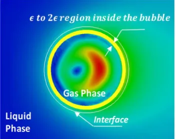
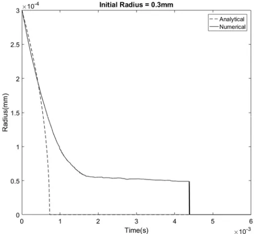
Figure 3.12. The comparison of bubble radius evolution in condensation simulation between analytical solution and numerical simulation. ... 57

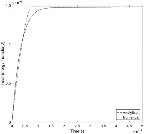
Figure 3.13. The evolution of energy transfer from the bubble to the surrounding liquid. ... 58

Figure 4.1. The schematic plot of contact angle calculation. ... 61

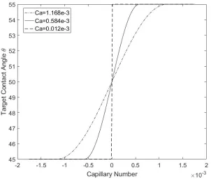
Figure 4.2. The schematic plot of target contact angle function. ... 63

Figure 4.3. The decision-making procedure for contact angle control modeling. ... 64

Figure 4.4. The schematic of contact angle control force application. ... 65

Figure 4.5. The schematic plot of F1 function. ... 66

Figure 4.6. Force balance analysis for the single bubble on the wall... 67

Figure 4.7. The mesh design of bubble departure case. ... 69

Figure 4.8. The bubble departure process for different target contact angle. The surface tension is equal to 0.0729N/m in the simulations. CA indicates the prescribed target contact angle. The color indicates the velocity magnitude field... 70

Figure 4.9. The contact angle evolution history for different target contact angles. CA indicates the prescribed target contact angle. ... 72

Figure 4.10. The contact angle evolution for critical contact angle simulation. ... 77

(17)

xiv Figure 5.1. The 3D domain and mesh design of single bubble growth with non-uniform

temperature distribution. ... 80

Figure 5.2. The evaporation and condensation snapshots (colored by the superheat field in

first column while velocity in second one). ... 82

Figure 5.3. The void fraction plot based on time step during bubble growth with

non-uniform temperature distribution (The circle indicates the data point of the

snapshots in Figure 5.2). ... 83

Figure 5.4. The initial temperature condition of single bubble growth and departure

simulation. ... 84

Figure 5.5. The mesh design and boundary condition of single bubble growth and departure

simulation. ... 85

Figure 5.6. The 3D zoomed figure of the boundary layer mesh in the pool boiling

simulation. ... 87

Figure 5.7. The simulated evolution of bubble growth and departure from the wall (The

temperature distribution is shown in row one and row three while the velocity

distribution is shown in row two and row four with interface contour). ... 88

Figure 5.8. The mesh design of single bubble growth and departure simulation for the mesh

sensitivity study (The bubble is represented by the white contour.). ... 89

Figure 5.9. The evolution of bubble equivalent radius over time for different meshes. ... 91

Figure 5.10. The mesh design of the domain and the schematic of the domain with the

artificial nucleation site. ... 92

(18)

xv Figure 5.12. The snapshots of bubble nucleating process. The background color indicates the

temperature distribution. ... 98

Figure 5.13. The evolution of bubbles nucleating from a single site. The background color

indicates the bubble ID field in BTA. ... 99

Figure 5.14. The comparison between the numerical result and the commonly-used

experimentally-based correlations. ... 100

Figure 5.15. The mesh design for the flow boiling simulation. ... 101

Figure 5.16. The temperature profile of flow boiling simulation that shows the bubble

movement in the center slice of the domain. The black line shows the interface.

... 103

Figure 5.17. The temperature profile of flow boiling simulation that shows the bubble

movement on bottom slice of the domain. Left side shows constant temperature

boundary condition; right side shows constant heat flux boundary condition. .... 104

Figure 5.18. The change of bubble volume along with time for the constant temperature

boundary condition and the constant heat flux boundary condition. ... 105

Figure 5.19. The estimated initial temperature profile compared with experimental

measurements. ... 107

Figure 5.20. The comparison between numerical flow boiling simulation and experimental

observation of bubble growth in flow boiling scenario (the time estimation refers

to simulation results) [102]. ... 111

Figure 5.21. The comparison of the bubble growth rate in the flow boiling scenarios. ... 112

(19)

xvi Figure 5.23. The fully developed velocity and temperature profile of single phase simulation.

The left picture is the distribution of velocity from the side view; the right

picture is the temperature distribution (the saturation temperature is 100℃). ... 115

Figure 5.24. The initial bubble positions in the domain. The temperature field is shown on

the top picture while the velocity field is shown on the bottom with the mesh

design in the background. ... 115

Figure 5.25. The results of multi-bubble flow boiling simulation. The snapshots show the

temperature distribution evolution. The contour in white line shows the bubble

interface. ... 119

Figure 5.26. The growth rate of each bubble in flow boiling. ... 120

(20)

xvii

LIST OF SYMBOLS AND ABBREVIATIONS Abbreviation

2D Two Dimensional

3D Three Dimensional

LWR Light Water Reactor

PWR Pressurized Water Reactor

DNB Departure from Nucleate Boiling

M-CFD Multiphase Computational Fluid Dynamics

DNS Direct Numerical Simulation

LOCA Loss-Of-Coolant Accident

HPC High-Performance Computing

ITM Interface Tracking Method

ONB Onset of Nucleate Boiling

CHF Critical Heat Flux

DFFB Dispersed Flow Film Boiling

OSV Onset of Significant Voids

LS Level-Set Method

CLS Conservative Level-Set

(21)

xviii FT Front Tracking method

VOF Volume Of Fluid

RANS Reynolds-Averaged Navier-Stokes (equations)

LES Large-Eddy Simulation

DES Detached Eddy Simulation

INS Incompressible Navier-Stokes (equations)

BTA Bubble Tracking Algorithm

MPI Message Passing Interface

GCI Grid Convergence Index

Notation

𝑃 Pressure inside the bubble (𝑃𝑎)

𝑃 Pressure in the surrounding liquid (𝑃𝑎)

𝑅 Radius of the cavity mouth (𝑚)

𝐷 Diameter of the largest cavities present on the surface (𝑚)

𝑇 Liquid bulk temperature (℃)

𝑁𝑎 Nucleation site density (𝑛𝑢𝑚𝑏𝑒𝑟/𝑚 )

𝑇 Wall temperature (℃)

(22)

xix 𝑡 Bubble growth time (𝑠)

𝑡 Bubble waiting time (𝑠)

𝐻 Smoothed Heaviside function

𝑑 Corrected distance field in the level set method (m)

𝑢 Instantaneous velocity component (𝑚/𝑠)

𝑢 Instantaneous velocity vector (𝑚/𝑠)

𝑤 Pseudo velocity vector (𝑚/𝑠)

𝑝 Static pressure (𝑃𝑎)

𝑡 Simulation time (𝑠)

𝑓 Body force component (𝑁)

𝑇 Absolution temperature of the fluid (𝐾)

𝑐 Specific heat at constant pressure (𝑘𝐽 (𝑘𝑔 ∙ ℃⁄ ))

𝑐 Specific heat at constant volume (𝑘𝐽 (𝑘𝑔 ∙ ℃⁄ ))

𝑆 Strain rate tensor

𝑘 Thermal conductivity (𝑊/(𝑚 ∙ 𝐾))

𝑇 Saturation temperature (℃ )

𝑞′′ Heat flux (𝑊/𝑚 )

𝑉 Volume of local element (𝑚 )

(23)

xx ℎ Latent heat of vaporization (𝑘𝐽/𝑘𝑔)

𝑅 Bubble radius (𝑚)

𝑛 The unit normal vector

𝐶𝑎 Capillary number

𝑉 Contact line speed (𝑚/𝑠)

𝐹 Contact angle control force (𝑁)

𝑑 Distance from the wall (𝑚)

𝐻 Height of the contact angle force application region (𝑚)

𝑇 Thickness of the contact angle force application region (𝑚)

𝑀 The offset of the arc-tangent function along the X axis

𝑌 The offset of the arc-tangent function along the Y axis

𝑦 The vertical distance from the bubble apex to the free surface (𝑚)

𝑥 The distance from the inlet to the nucleation point (𝑚)

∆𝑇 Liquid subcooling (℃)

∆𝑇 Liquid superheat (℃)

∆𝑇 Wall superheat (℃)

𝑈 Bulk liquid velocity (𝑚/𝑠)

𝑃𝑟 Prandtl number

(24)

xxi 𝐽𝑎∗ _{The normalized Jakob number}

𝑓 Bubble release frequency (1/𝑠)

Greek letters

𝜌 Liquid density (𝑘𝑔/𝑚 )

𝜌 Gas density (𝑘𝑔/𝑚 )

𝜀 Interface half-thickness in the level set equation (𝑚)

𝜀 Interface half-thickness in the re-distancing equation (𝑚)

𝜀 Interface half-thickness for bubble tracking algorithm (𝑚)

𝜇 Liquid dynamic viscosity (𝑁 ∙ 𝑠/𝑚 )

𝜇 Gas dynamic viscosity (𝑁 ∙ 𝑠/𝑚 )

𝜈 Liquid kinematic viscosity (𝑚 /𝑠)

𝜑 Level set scalar variable (𝑚)

𝜏 Reynolds stress tensor (𝑁/𝑚 )

𝜃 Dynamic Contact angle (°)

𝜙 Distance from the interface (𝑚)

𝛷 Static contact angle (°)

𝜃 Advancing contact angle (°)

(25)

xxii 𝜎 Surface tension (𝑁/𝑚)

𝜏 Pseudo time in re-distancing equations (𝑠)

𝛽 The bubble growth rate constant

𝛼 Liquid thermal diffusivity (𝑚 /𝑠)

𝛿 Thermal boundary layer thickness (𝑚)

𝛿 Hydrodynamics boundary layer thickness (𝑚)

𝛿 The average thickness of the microlayer (m)

(26)

1

CHAPTER 1.INTRODUCTION

1.1. Overview and Motivation

Boiling phenomenon accommodates large heat fluxes with relatively small driving

temperature difference, which makes it ideal for applications that demands substantial heat transfer

rates like Light Water Reactor (LWR) nuclear power plants, chemical thermal processing, heat treatment and manufacturing, microelectronic cooling, and numerous microscale devices

(microelectromechanical systems, micro heat pipes, lab-on-chips, etc.). The distribution of steam

in a boiling mixture affects the heat transfer rate and may cause unfavorable conditions. For

example, the distribution of vapor in the LWR sub-channels can cause burn-out phenomenon at

certain wall superheat known as Departure from Nucleate Boiling (DNB). DNB, in turn, may cause fuel cladding damage, which may lead to reactor unplanned shutdowns and even accidents. Due

to its complex nature, better understanding and modeling of boiling process remains a major

challenge in multiphase flow research. In the last eight decades, boiling phenomenon has been an

enduring appeal to researchers. The modeling of two-phase boiling phenomena has evolved a wide

range of approaches, from one-dimensional models, to quasi-multidimensional subchannel

models, to three dimensional Multiphase Computational Fluid Dynamic (M-CFD) models, and recently to Direct Numerical Simulations (DNS) of multiphase flows where individual bubbles are fully resolved.

The one-dimensional models (e.g., homogeneous equilibrium models, phasic slip models,

drift-flux models and two-fluid models) are widely used in system thermal hydraulics codes such

as RELAP5[1], TRACE [2] and GOTHIC [3]. This type of simulations is used by the nuclear

community to analyze various reactor transients and accident scenarios Loss-Of-Coolant Accident

(27)

2 rods) models are utilized by subchannel analysis codes like COBRA-TF [4] to evaluate nuclear

reactor safety margins. However, simulations based on one-dimensional models and

quasi-multidimensional subchannel models do not resolve the anisotropy in the coolant channel and

completely rely on single- and/or two-phase closure correlations. Many of the closure correlations

in these models are only valid for specific geometries and a limited range of fluid dynamics and

heat transfer conditions. If the application regions from different correlations do not satisfactorily

overlap with each other in the simulation, their predictive capability may degrade when applied to

new scenarios.

The advances in High-Performance Computing (HPC) in recent years make it possible to apply M-CFD to a wide variety of bubble hydrodynamics and thermodynamics studies [5, 6]. The

M-CFD method can resolve thermal and velocity fields adjacent to the wall boundaries and the

void fraction within three-dimensional domain representing the flow geometry. Therefore, this

type of simulations could provide detailed information about the location of vapor generation

onset, axial temperature profile, and axial and radial void distribution in two-phase flow [5].

However, simulations based on the M-CFD models require certain interfacial exchange terms

(including mass, momentum and energy exchanges) to obtain closure like the lift force [7], the

turbulent dispersion force [8], the wall heat flux partitioning [9], etc. In addition, the development

and validation of 3D M-CFD model and physics-informed data-driven modeling require data of

high-quality and high-resolution. Considering the difficulties in acquiring the corresponding

experimental data in prototypic conditions, two-phase simulations based on DNS approach

becomes feasible for many engineering applications.

In recent years, the DNS approach has already shown to be a reliable data source for model

(28)

3 (ITM) is coupled with a DNS solver, the instantaneous velocity and temperature field at, and

around, the interface, which may not be straightforward to obtain by any of the methods discussed

above, can be calculated in two-phase flow simulations. ITM approach provides not only detailed

physics-based description associated with thermal and hydrodynamic processes but also the shape

of the evolving interface. A number of simulations utilized ITM approach have been conducted

for bubble dynamics and heat transfer problems [12-18]. However, the ITM boiling models have

been proposed so far are all developed for 3D structured mesh or 2D unstructured mesh. Both

types of ITM boiling models face extreme difficulties when applying to large scale boiling

simulation with complex geometries. The 2D ITM boiling models doesn’t have correct

representation of 3D bubbles. The 3D ITM boiling model for structured mesh has been

successfully applied to various boiling scenarios, but it requires huge amount of computation

resource to accurately simulate the scale changes from nucleate bubble to high void fraction

regime. In addition, the structured grid requirement makes it challenging to apply in complex

engineering geometries. So, most ITM boiling models in the literature mainly focus on the boiling

simulation in limited domains (e.g. single coolant channel, small water pool) and the fundamental

study of the boiling heat transfer mechanism. Meanwhile, other simulation approaches studying

the system thermal hydraulic in large scale cannot provide detailed information at and around the

bubble interface and rely on highly empirical closure models. The ITM boiling model in this

research aims to fill the numerical data gap between the study of local phenomenon and the large

scale engineering application by performing high resolution high quality large scale boiling

simulation in practical geometries. In order to perform large scale boiling simulation, the ITM

boiling model is developed in consideration of conducting simulations with local mesh refinement,

(29)

4 This work focuses on the development, verification and validation of this 3D ITM boiling

model and, also demonstrate the potential of this model in conducting large scale boiling

simulation for engineering applications. The boiling simulations in the presented research are

conducted in full 3D representation with the unstructured grid. This approach allows us to

investigate the boiling phenomenon in various conditions with lower cost (by utilizing local mesh

refinement for bubble growth region). The bubble dynamics information including bubble

trajectory, growth rate, etc. is collected individually for each bubble using the modified and

improved bubble tracking algorithm (BTA) [19]. Together with the massively parallel-computing

capability of PHASTA (which is the advanced flow solver used for the presented research, and the

abbreviation stands for Parallel, Hierarchic, higher-order accurate, Adaptive, Stabilized, Transient

Analysis), this work enables the high-resolution boiling simulations in subchannel scale (Appendix.B), including the challenging prototypic pressure/temperature conditions existing

(30)

5

1.2. Boiling Regimes

Steam-water two-phase mixture can form a lot of different topological interface flow

configurations. The two-phase boiling regimes summarized the most frequently observed flow

pattern in boiling phenomenon. The ranges of occurrence of the major two-phase flow regimes are

essential for the modeling and analysis of two-phase boiling systems. The frequently-used pool

boiling and the flow boiling regimes are discussed in this section.

1.2.1. The Pool Boiling Regimes

The distribution of vapor in a boiling mixture forms various bubble topologies at different

applied wall heat flux, which affects the heat transfer rate and flow dynamics of the system. The

flow regime maps are introduced to quantify visually observed flow patterns in terms of measured

quantities, so that the existence of a certain flow regime, or the transition from one flow regime to

another can be predicted. For each flow regime, the dominating heat transfer mechanism and flow

characteristics are different. In most system thermal hydraulics codes, the flow regime is an

important criterion for heat transfer model selection. The different heat transfer mechanisms are

often represented by a boiling curve. The typical version of the pool boiling curve [20] is shown

in Figure 1.1 and was originally introduced by Nukiyama [21] to describe the relation between the

wall heat flux and the wall superheat (the difference between wall temperature and the saturation

temperature at system pressure). In the first region, heat transfer is dominated by natural

convection and the energy accumulated at the vicinity of the heated surface is not enough to initiate

nucleation. As the heat flux and the wall superheat increases, at one point the nucleation site starts

to be active and bubbles appear on the heated surface, which is known as the Onset of Nucleation Boiling Point (ONB). In the partial nucleate boiling region, isolated bubbles nucleate, grow, depart, slide along the wall and eventually lift off. The heat transfer is dominated by a complex

(31)

6 nucleation sites are activated, and the isolated bubbles grow larger and merge with other bubbles

to form vapor columns and mushroom-shaped bubbles, which is known as fully developed

nucleate boiling. In this region, the fraction of the wall surface area subject to nucleate boiling

increases until bubble formation occupies the entire heated surface and the contribution of natural

convection heat transfer is negligible. As bubble density increases, bubbles start to coalesce and

form heat-insulating vapor films, which also impedes liquid return back to the surface. The heat

transfer rate under this condition reduces dramatically. This point C is called Critical Heat Flux

(CHF). Further increase in the wall heat flux leads to the post CHF boiling regimes: transition

boiling and film boiling. In transition boiling region, the vapor films grow, and collapse

dynamically. As the wall superheat increases, the dry fraction of the heated surface increases. As Figure 1.1. Typical pool boiling curve and associated flow regimes[20].

(32)

7 more and more wall surface covered by vapor film, the film boiling is achieved. There is no direct

macroscopic contact between liquid and solid surface. The heat transfer coefficient decreases

significantly compared to that of nucleate boiling due to conductivity, density and heat capacity

properties of vapor.

Of these three boiling modes, film boiling is the easiest to analyze. The nucleate and transition boiling are much more complex and usually require empirical or mechanistic

correlations as model closures.

1.2.2. The Flow Boiling Regimes

Flow boiling is considerably more complicated than pool boiling due to the coupling

between flow hydrodynamics and boiling heat transfer processes. As the void fraction increases

during flow boiling, the two-phase and boiling heat transfer regimes are developing along the

heated channels. The configuration of the boiling channel also affects the heat transfer rate and the

flow regime transition. The vertical upflow channel is often used in many thermal cooling systems

(e.g. LWR coolant channel) since the buoyancy effect in such configuration can help the flow of

the mixture which in turn improves the heat transfer rate. It is noted that the horizontal boiling

channels and vertical downflow channels are also of interest in certain operating conditions.

The schematic flow boiling regimes are displayed in Figure 1.2. The two-phase flow

patterns develop in a vertical upflow channel with uniform and moderate heat flux. When the inlet

flow has a large subcooling, the entire flow channel remains to be subcooled. If the wall heat flux

increases, the first bubble will form at some location downstream where the wall superheat is high

enough to initiate nucleation. The flow regime at the exit can be bubbly flow, slug flow or annular

(33)

8 the boiling will start at the inlet region and has a large chance moving to Dispersed Flow Film Boiling (DFFB) regime and the single-phase pure vapor flow regime.

The subcooled flow boiling covers the region beginning from the location where the wall

temperature exceeds the local liquid saturation temperature to the location where the

thermodynamic quality reaches zero, corresponding to the saturated liquid state. There are three

regions of subcooled flow boiling identified by earlier researchers as: (i) single-phase forced

convection region, (ii) partial nucleate boiling, and (iii) fully developed nucleate boiling. A

schematic representation of the subcooled flow boiling is shown in Figure 1.3. The inlet flow is

highly subcooled. There is no volume fraction of vapor and the heat transfer is dominated by

single-phase forced convection. At some location downstream, bubbles start to nucleate because

of the local wall superheat while the bulk liquid is still subcooled. This location is identified as the

(34)

9

Onset of Nucleate Boiling (ONB). Downstream of ONB, the bubbles are still small enough to remain attached to the heater surface. As the bulk liquid temperature increases, the bubbles grow

larger, begin to depart from the nucleation sites, slide along the heater surface, and eventually lift

off from the wall. The location where the bubbles begin to lift off from the heated wall is called

the location of Onset of Significant Voids (OSV). In the region between ONB and OSV, the void fraction is small but increases rapidly downstream of OSV. The heat transfer mechanism is a

complex mixture of single-phase forced convection, evaporation, condensation and quenching. As

the void fraction increases, a bubbly layer may form adjacent to the wall and eventually develop a

thin film layer between the liquid and the heated wall surface. This leads to the Departure from Nucleate Boiling (DNB) event. The heat transfer coefficient deteriorates dramatically downstream from this point. In nuclear reactor, DNB may cause fuel cladding damage and result in reactor

(35)

10

1.3. Heterogeneous Bubble Nucleation and Active Nucleation Sites

The defects of the heated surfaces like microscopic/nanoscopic cavities and crevices can

trap minute pockets of air when the surface is submerged in the liquid. These pre-existing interface

areas act as an embryo for bubble growth under low heat flux conditions. This phenomenon is

referred to as heterogeneous bubble nucleation. Compared to homogenous boiling which requires

large liquid superheats to initiate the nucleation process, heterogeneous boiling only needs a few

degrees of wall superheat. Nucleation on the defects of the heated wall surface can take place

within a thin, superheated liquid layer adjacent to the wall while the liquid bulk is subcooled. Hsu

[22] was the first to propose the criteria for boiling inception. According to their experimental

results[23], the liquid layer surrounding the embryo must be equal or larger than the saturation Figure 1.3. Two-phase subcooled flow boiling regime with a moderate and uniform wall heat

(36)

11 temperature at the corresponding pressure for bubble growth. The pressure difference between

bubble interior and surrounding liquid can be expressed by Young-Laplace equation (∆𝑃 =

2𝜎/𝑟 ). The Clausius-Clapeyron relationship, a bubble surrounded by a liquid with uniform

temperature, was written in terms of temperature as,

𝑇 − 𝑇 ≈ 𝑇

𝜌 ℎ (𝑃 − 𝑃 ) =

2𝑇 𝜎

𝜌 ℎ 𝑅 ( 1-1 )

where 𝑇 is the temperature of the surrounding liquid, 𝑃 is the pressure inside the bubble, 𝑃 is the

pressure in the surrounding liquid and 𝑅 is the radius of the cavity mouth.

Assuming a linear temperature profile in the thermal boundary layer with thickness 𝛿 as,

According to Hsu’s criteria, the possible range of nucleating cavity size for a certain wall superheat

is given,

where 𝐶 = 1 + 𝑐𝑜𝑠𝜃 and 𝐶 = 𝑠𝑖𝑛𝜃 when the cavity mouth has a slope of 𝜃 , 𝑇 is the wall

surface temperature and 𝑇 is the liquid bulk temperature.

Several improvements have been introduced into Hsu’s criterion [22]. Howell and Siegel

[24] argued that Hsu’s criterion is conservative. The temperature measured in their experiments

turned out to be lower than the temperature requirements of Hsu’s criterion. They proposed to use

net heat exchange rate between the bubble and surrounding liquid for bubble growth. Wang and

Dhir [25] provided a minimum superheat required to initiate nucleation based on the minimization

of the Helmholtz free energy of a system containing a gas-liquid interphase for highly wetting

liquids. They derived the inception criterion for a spherical cavity as following [26], 𝑇 (𝑦) − 𝑇

𝑇 − 𝑇 = 1 − 𝑦/𝛿 ( 1-2 )

𝑅 , , 𝑅 , = 𝛿𝐶 2𝐶

𝑇 − 𝑇

𝑇 − 𝑇 × 1 ∓ 1 −

8𝐶 𝜎𝑇 (𝑇 − 𝑇 )

(37)

12 where

where 𝜃 is the interface contact angle measured in the liquid side.

Basu et al. [27] expanded the minimum superheat criterion by accounting for the

wettability of commercial surface whose cavity shape and size distribution are hard to determine.

They concluded that the minimum wall superheat required diminishes as the wettability increases

(the contact angle decreases). Most recently, the BETA experimental results by Theofanous et

al.[28] indicated that the micron-scale and macroscopic roughness may not be necessary for

heterogeneous nucleation and parameters such as cavity size, or contact angle are of derivative

significance in heterogeneous boiling. The discussion on the heterogeneous nucleation is on-going

in the research community and the principal cause/mechanism still remains to be found.

The nucleation sites density describes the number of bubbles that are found (at any time)

per unit area of the heater surface, which is another important integral characteristic of

heterogeneous nucleation boiling. Mikic and Rohsenow [29] assumed that the number of sites per

unit area with radii larger than 𝐷 /2 can be approximated with the power law:

𝑁 = 𝐷

𝐷 ( 1-6 )

where 𝐷 is the diameter of the largest cavities present on the surface and 𝑚 is an empirical

constant. The nucleating cavity diameter 𝑅 (The same 𝑅 in Eq.( 1-1 )) can be related to fluid

properties and wall superheat ∆𝑇 as:

𝑇 − 𝑇 = 2𝜎𝑇

𝜌 ℎ 𝑅 𝐾 ( 1-4 )

𝐾 =

1 𝑓𝑜𝑟 𝜃 ≤𝜋 2 sin 𝜃 𝑓𝑜𝑟 𝜃 >𝜋

2

(38)

13 where 𝜎 is the liquid surface tension, 𝜌 is the vapor density and ℎ is the latent heat of

evaporation.

Kocamustafaogullari and Ishii [30] proposed another nucleation site density model which

was correlated to the dimensionless minimum cavity size and the fluid density ratio. The boiling

heat transfer data used in their model covered a wide range of pressure variation. The bubble

dynamics and heat transfer in the region between nucleation sites were also considered in the

nucleate boiling heat transfer calculation. Therefore, their model has a fairly good representation

of the existing experimental water data.

𝑁∗ = [𝐷∗ . 𝐹(𝜌 ∗)] / . ( 1-8 )

where

𝑁∗ = 𝑁 𝐷 ; 𝐷 = 𝐷 𝐷⁄ ; 𝜌∗ = (𝜌 − 𝜌 )/𝜌 ( 1-9 )

and

In Eq.( 1-9 ), the bubble diameter at departure 𝐷 is obtained by Fritz’s correlation [31],

and the nucleating cavity diameter 𝐷 is obtained using Eq. ( 1-7 ) at low to moderate pressures.

Basu et al. [32] proposed a model that correlated nucleation site density to contact angle

values. According to their results, the correlations for the nucleation site density were independent

of flow rate and liquid subcooling but dependent on the contact angle and wall superheat. 𝑅 = 4𝜎𝑇

𝜌 ℎ ∆𝑇

( 1-7 )

𝐹(𝜌∗_{) = 2.157 × 10 𝜌}∗ . _{(1 + 0.0049𝜌}∗₎ . _{( 1-10 )}

𝑁 = 3.4[1 − cos 𝛷]∆𝑇 ∆𝑇 _, ≤ ∆𝑇 < 15℃

𝑁 = 3.4 × 10 [1 − cos 𝛷]∆𝑇 . _{∆𝑇 > 15℃}

(39)

14

1.4. Bubble Growth Model

Researchers have attempted to model bubble growth in nucleate boiling since the 1950’s.

In the early growth models, the bubble is assumed to be surrounded by superheated liquid and the

bubble growth is driven by the evaporation at the interface. Plesset and Zwick [33] and Forster and

Zuber [34] derived analytical bubble growth models for bubbles surrounded by uniformly

superheated liquid. Researcher like Birkhoff et al.[35] and Scriven [36] improved this analytical

model and Mikic et al.[37] extended the analytical growth model to non-spherical bubble.

However, this type of bubble growth model does not account for the wall effect on the

bubble growth. When a bubble grows from the nucleation site, it is believed that there is a thin

liquid layer (the microlayer) underneath the bubble. As the microlayer evaporates, an initial sharp

drop in temperature occurs and a recovery in the temperature happens after formation of a dry spot.

After this a small drop in temperature and subsequent recovery appears when liquid rewets the

surface during the bubble departure. The existence of micro-layer underneath the growing bubble

has been confirmed via local temperature distribution measurements. Moore and Mesler [38]

observed the significant local temperature fluctuations on the wall under the bubbles during the

nucleate boiling and suggested that microlayer evaporation could be the reason of the fluctuations.

Hendricks and Sharp [39] correlated the wall temperature fluctuations with high-speed videos of

individual bubbles and showed that the rapid temperature decrease in the wall temperature was

associated with bubble growth. Cooper and Lloyd [40] measured the temperature field evolutions

during boiling of toluene and isopropyl alcohol on the glass and ceramic substrates whose

backsides were radiantly heated. They proposed the average thickness of the microlayer can be,

where 𝐶 ≈ 0.3 − 1.3, 𝑡 is the bubble growth time and 𝜈 is the kinematic viscosity of liquid.

(40)

15

1.5. Bubble Departure Diameter

There is a large volume of published studies describing the diameter to which a bubble

grows before departure. Fritz [31] proposed a correlation based on the force balance between

buoyancy force, which acted to lift the bubble from the surface, and the surface tension force,

which tended to hold the bubble to the wall in pool boiling condition. The resulting bubble

departure diameter is given as

where 𝛷 is the static contact angle measured in degrees. Han and Griffith [41] found that the Fritz

formula worked as long as the true (no-equilibrium) bubble contact angles were used. In general,

these values should be known for various fluids at different pressure. However, these data of

bubble contact angles reported in literature are very limited and inconsistent. For example, Griffith

and Wallis [42] found that the average value of Φ(contact angle) did not depend on water

saturation pressure while Labuntsov et al.[43] showed that there was a weak effect of the saturation

pressure on Φ for water boiling on a silver surface at 𝑝 = 0.1 − 15𝑀𝑃𝑎. Pioro et al.[44]

suggested that the task of obtaining accurate values of the true contact angle during boiling was

unrealistic. Therefore, the Fritz formula can only be considered as a theoretical approach. In

general, part of the formula

( ) is used in many practical non-dimensional correlations

for nucleate pool boiling heat transfer calculation. Some of the wide-used correlations are shown

below.

Cole and Rohsenow [45] correlated bubble departure diameter at low pressures as 𝐷 = 0.0208Φ 𝜎

𝑔(𝜌 − 𝜌 ) ( 1-13 )

𝐷 = 1.5 × 10 𝜎

𝑔(𝜌 − 𝜌 )𝐽𝑎

(41)

16 and

𝐷 = 4.65 × 10 𝜎

𝑔(𝜌 − 𝜌 )𝐽𝑎

∗ / _{for other liquids} _{( 1-15 )}

where Ja∗ = 𝜌 𝑐 𝑇 ⁄𝜌 ℎ is the normalized Jakob number. Kocamustafaogullari [46]

proposed a correlation for bubble departure diameter including high-pressure conditions as below:

𝐷 = 2.64 × 10 𝜎 𝑔(𝜌 − 𝜌 )

𝜌 − 𝜌 𝜌

.

( 1-16 )

It is widely agreed that

( ) is proportional to the bubble departure diameter, but a

generalized correlation (a correlation could be used for both low pressure and high pressure) or

comprehensive model for bubble departure diameter has not been proposed yet. The key

impediments have been the lack of knowledge of instantaneous local velocity and temperature

field. The velocity and temperature field vary both temporally and spatially because of bubble

deformation and bubble movement. This, in turn, affects the bubble growth rate and forces that act

on the bubble through temperature and velocity fields. Additionally, surface wettability,

contribution of microlayer, and merger of vapor bubbles have an influence of bubble departure

(42)

17

1.6. Bubble Release Frequency

The time period before bubble released is categorized into growth time and waiting time

for modeling purpose [47]. The growth period is defined as the time from the nucleation occurs to

the bubble lifts off, which are mainly affected by the bubble evaporation rate and bubble departure

diameter. The waiting time describes the time needed for the new bubble appears at the same

nucleation site after the previous one departs. Once the bubble lifts off from the wall, the cooler

liquid in the vicinity rushes in to fill the space previously occupied by the vapor. Most waiting

time models assumed that the nucleation site would be activated once the liquid superheat

condition was established. Hsu and Graham modeled the liquid thermal field as one-dimensional

transient conduction in a slab and proposed a waiting time model 𝑡 as follows [23, 48],

where 𝛼 = 𝑘/𝜌𝑐 is the thermal diffusivity of liquid and 𝑅 is the cavity size. However, the local

cooling of the solid is ignored in this model. The thermal response of the solid surface was taken

account later by Hatton and Hall [49].

Bubble release frequency reflects the number of bubbles released from the same nucleation

site per unit time. It is defined as the inverse of the summation of the growth and waiting time.

One of the commonly used correlations was proposed by Zuber [50] as,

𝑓𝐷 = 0.59 𝜎𝑔(𝜌 − 𝜌 ) 𝜌

/

( 1-18 )

Jakob and Fritz [51] proposed that the product of bubble release frequency (𝑓) and bubble

departure diameter (𝑓𝐷 ) should be a constant,

𝑓𝐷 = 0.078 ( 1-19 )

𝑡 = 9 4𝜋

(𝑇 − 𝑇 )𝑅

𝑇 − 𝑇 1 −_{𝑅 𝜌 ℎ}2𝜎

(43)

18 Cole’s correlation of bubble release frequency is also well known for pool nucleate boiling,

𝑓 = 4𝑔(𝜌 − 𝜌 ) 3𝐷 𝜌

( 1-20 )

Here 𝐷 in the correlations above denotes the bubble departure diameter (discussed in Section 1.5)

There are other correlations proposed for bubble release frequency. Mikic and Rohsenow [29]

developed a model for heat-transfer-controlled growth of a bubble in a non-uniform temperature

field near a heated surface. The bubble release frequency is derived using the waiting and growth

times,

where 𝐷 is the departure diameter, 𝛼 is the thermal diffusivity (= 𝑘 𝜌𝑐⁄ ), 𝐽𝑎 is the Jakob

number defined as,

𝐽𝑎 =𝜌 𝑐 [𝑇 − 𝑇 (𝑝 )] 𝜌 ℎ

( 1-22 )

However, predictions from these correlations are valid only for the limited data range over

which supporting data have been obtained. It is hard to model bubble release frequency because

all the parameters in nucleate boiling like bubble growth rate, temperature and velocity field in the

vicinity of the bubble, heater response, etc. are interrelated. Innovative approaches in experiments

and simulations are needed to help the mechanistic model development for this complex

phenomenon. 𝑓 / 𝐷 = 4

𝜋 𝐽𝑎 3𝜋𝛼

𝑡 𝑡 + 𝑡

/

+ 1 + 𝑡 𝑡 + 𝑡

/

(44)

19

1.7. Bubble Contact Angle

During the nucleate boiling process, a vapor bubble nucleates from a micro-cavity in the

wall surface, grows due to the wall at superheat temperature, and departs when it reaches a critical

size determined by a local force balance. Previous research has shown that contact angle plays an

essential role in determining boiling parameters like nucleation site density [52], bubble departure

diameter [31], and bubble release frequency [50]. Therefore, it is important to maintain correct

contact angle in boiling simulations. The contact angle used in boiling models is defined as the

angle between the vapor-liquid interface at the interface contact line and the wall surface in liquid

side as shown in Figure 1.4. The advancing contact angle (𝜃 ) is the maximum value of the

contact angle at the interface contact line while the receding contact angle (𝜃 ) is the minimum

value. If the wall surface is ideal (smooth, flat, and homogenous) and the interface is not moving,

the contact angle only depends on the vapor and liquid properties and the solid surface material.

In this situation the contact angle is defined as the static contact angle. As the bubble grows or

slides along the wall, the bubble movement will have an impact on the value of contact angle

besides physical properties and surface material. This type of scenarios is described using dynamic

(45)

20 contact angle, and typically requires specification of advancing and receding contact angles. One

must note, that the static contact angle usually does not have a well-defined value for realistic

surfaces, because most surfaces are not ideal. Typically, a measured dynamic contact angle value

would fall into the interval between the advancing contact angle and receding contact angle.

The contact angle hysteresis has been studied for various solid-liquid combinations and

surface conditions. Young [53] was one of the first researchers to recognize the relationship

between surface tension and contact angle. By analyzing the contact angle of a gas bubble on a

solid surface in the water, he suggested that the contact angle was determined through the balance

of the surface tension forces between the three material phases: gas, liquid and solid. However, it

is noted that the validity of Young’s model requires the solid surface to be ideal, which is almost

impossible to achieve in practice. Wenzel [54] investigated the effect of the roughness of the

surface on the static contact angle. His research demonstrated that surface roughness enhanced the

hydrophobic effect — if the fluid was hydrophobic: it would behave more hydrophobic on the

rough surface than it on the smooth surface. Similar effect was observed for hydrophilic fluids:

this property was also enhanced on rough surfaces. Cassie [55] proposed a model describing the

changes of the contact angle on a heterogeneous surface. Lam et al. [56] measured the dynamic

one-cycle and cyclic contact angle for various liquid/solid combinations. They recognized four

different patterns of receding contact angle behavior in their experiments.

Besides the surface conditions of liquid-solid combination and physical properties of each

phase, the contact angle is also influenced by the vapor-liquid interface velocity. Ramanujapu and

Dhir [57] experimentally investigated nucleate pool boiling phenomenon and focused their efforts

on the dynamic contact angle measurements at the base of vapor bubbles. Their results showed

(46)

21 a weak dependency on the interface velocity in the performed range of experiments. Sobolev et al.

[58] conducted measurements of the dynamic contact angle of water in the thin quartz capillaries

with various radii in the range of 40 to 200 nm. They found that the dynamic contact angle is

linearly dependent on the velocity when velocities were less than 5 μm/s while it is independent

at higher velocities. Kandlikar et al. [59] experimentally investigated an evaporating meniscus on

a smooth moving heated surface. They concluded that the contact angle was almost independent

of the wall superheat for the stationary meniscus and as the surface velocity increased the receding

contact angle would vary at relatively low wall superheat. The advancing and receding motion of

the meniscus increased the local heat transfer rate, which is observed in the experiment.

Several different models of dynamics contact angle have been proposed for numerical

simulations. Fukai et al. [60] experimentally and theoretically investigated the deformation of a

liquid droplet impacting against a flat surface. In their presented model of the wetting effect, the

dependency of contact line velocity and the distinct value of advancing and receding contact angle

were considered. The contact angle values were determined experimentally and used as input to

the model. The numerical prediction of droplet shape evolution showed qualitative agreement with

the measured data. Bussman et al. [61] proposed a 3D model to describe the impact of a droplet

on asymmetric surface geometries using volume tracking algorithm. Contact angle model was

applied as a boundary condition at the contact line. In their method, the advancing and receding

contact angles obtained from the experiments were applied to the contact angle model if the

simulated contact line velocity was greater than specified velocity criteria (0.1 m/s). At the

locations where the contact line velocity was less than velocity criteria (0.1 m/s), the contact angle

(47)

22 in the range where the contact line velocity value is less than velocity criteria were also specified

as a constant equilibrium contact angle.

Abarajith and Dhir [62] numerically investigated the effect of contact angle on the single

bubble during nucleate pool boiling using Level-Set method (LS). The contact angle was maintained at a constant value during the bubble growth and departure process. As the contact

angle increased, the bubble departure diameter and time to departure both increased. The

simulations were carried out on the two-dimensional and axisymmetric domain in their study. Son

and Hur [63] proposed a contact angle model on non-orthogonal grids for LS. The 2D and 3D

simulations of free-surface motions were conducted, but only 2D simulations were performed for

the motion of the droplet on an inclined wall. Mukherjee and Kandlikar [64] studied single bubbles

with dynamic contact angle during nucleate pool boiling using LS. They proposed a dynamic

contact angle model which linked the dynamic contact angle to the contact line velocity. A similar

approach is adopted in the contact angle algorithm for the presented high-resolution boiling

simulations research, where the contact angle is expressed as a function of contact line velocity.

According to their results, the decrease in surface wettability played a key role in departing a

bubble with a larger diameter. The simulations were performed using three-dimensional structured

meshes. Sato and Niceno [65] came up with a contact line treatment for a Conservative Level-Set

(CLS) method. The contact angle model was implemented as a special type of boundary condition.

The 3D simulations including droplet on a wall without gravity and bubble detached from the wall

(48)

23

1.8. Interface Tracking Boiling Simulations

In recent years, there has been an increasing interest in applying DNS to boiling

simulations. The DNS approach has already shown to be a reliable data source for model

development and validation of single-phase flow [10]. After an Interface Tracking Methods (ITM) are introduced to a DNS-capable solver, the conservation equations of mass, momentum, and

energy for liquid and vapor phases are solved simultaneously using one-fluid approach as the

interface is continuously evolving at/near the heated surface. The instantaneous velocity and

temperature field at, and around, the interface, which may not be straightforward to obtain by any

of the methods discussed above, can be calculated in two-phase flow simulations. There are

different types of ITM including Marker and Cell (MAC) method [66], Front Tracking (FT) Method, Level-Set (LS) method, Volume-Of-Fluid (VOF), and several others. MAC method uses massless particles to track interface movement and reconstruct the interface in the structured mesh.

One of the earliest boiling simulation based on the MAC method was done by Madhaven et al.

[67]. Similar to the MAC method, FT method also utilized massless particles to follow the interface

movement, but the interface is tracked using Lagrangian method and the particles are always

connected through a separate computational grid [68]. Tryggvason et al. [68] developed and

improved this method, especially the curvature calculation. His research group conducted a series

of boiling-related simulation using FT method [69-71]. The LS method introduces a distance field

(level-set field) that contains the information about the distance to the interface which is set to be

zero level set [72-74]. Dhir and his group [18, 75, 76] have conducted various boiling simulations

using LS method. The detailed simulations will be discussed later in this section. The level-set

method is also utilized in Bolotnov’s research group [77-80] for bubble dynamics and heat transfer

(49)

24 reconstructs the interface based on the volume fraction information [81]. Kunugi et al. applied this

method to subcooled pool and flow boiling simulations [82, 83].

The Level-Set simulation on boiling phenomenon has started at the end of 1990’s. Most of

the boiling simulations at that time were done in a 2D domain with structured mesh. One of the

early research efforts on 2D numerical boiling simulation was conducted by G. Son et al. [16]

simulating a growing and departing bubble on a horizontal surface. The local wall heat flux and

the effect of microlayer evaporation are considered in their simulation. The bubble merger process

was studied by Son et al. [18] on a single nucleation site during pool nucleate boiling. The level

set method was used to handle breaking and merging of the interface and modified to include the

effects of phase change at the interface and contact angle at the wall. As the capabilities of HPC

grow, the 3D boiling simulation with interface tracking methods became feasible. A. Mukherjee

and V.K. Dhir [17] conducted 3D simulations of the lateral merger of vapor bubbles during

nucleate pool boiling. Calculations were carried out for multiple bubble mergers in a line and in a

plane using uniformed structured mesh. Their results showed that the merger of multiple bubbles

significantly increased the overall wall heat transfer. Gihun Son and V.K. Dhir [15] investigated

nucleate boiling on a horizontal surface at high heat flux including the effect of wall superheat, the

number density of active nucleation sites and waiting period on the bubble dynamics and heat

transfer. Sato and Niceno [14] performed a nucleate pool boiling simulation on the boiling regime

from discrete bubble to vapor mushroom regime. Both the conjugate heat transfer phenomenon

and the vaporization of the micro-layer were considered in their simulations. Compared with pool

boiling, only a few simulations focus on flow boiling phenomenon. Li and Dhir [84] performed a flow boiling simulation with a single bubble in the rectangular shape domain in 2007, but the

(50)

25 one-half of the domain was simulated, and the three-dimensional domain was obtained by the

planar symmetry of the geometry. Dahiri and Tryggvason [12] simulated the heat transfer in

turbulent bubbly flow in vertical channels, but bubble evaporation and condensation were not

considered in their simulation. Almost all these simulations are conducted in cuboid or tube-like

domain with structured mesh. Despite the reduced cost of computational resources, 3D boiling

simulation with interface tracking method, especially for engineering applications, remains

relatively expensive. The need of increasing the affordability of simulations by improving

(51)

26

1.9. Research Objectives

The development and validation of 3D Multiphase Computational Fluid Dynamics (M-CFD) model and physics-informed data-driven modeling require data of quality and

high-resolution. Considering the difficulties in acquiring the corresponding experimental data in

prototypic conditions, two-phase simulations by ITM-based models can be used for generating

high-resolution numerical data in a consistent, best-estimate, and relatively economical manner.

The development, verification and validation of a boiling model in one of the ITM-based

multiphase-flow solvers, named PHASTA, is presented in this dissertation: (a) The evaporation

and condensation model is designed for multiphase simulations in full 3D representation with the

unstructured grid. This model is capable to investigate the boiling phenomenon under various

conditions with lower cost (by utilizing local mesh refinement for bubble growth region); (b) The

contact angle control model is implemented to maintain correct contact angle while the bubble is

attached to the wall; (c) The bubble dynamics information including bubble trajectory, growth rate,

etc. is collected individually for each bubble using the modified and improved bubble tracking

algorithm [19]. This unique capability can help improve multiphase computational fluid dynamics

models and perform virtual experiments on the much larger scale (billions of mesh cells on tens

of thousands of computing cores) like subchannel geometry under PWR temperature / pressure

normal operating conditions.

To better present the model development approach, verification, validation and application

examples, this dissertation is structured as follows: CHAPTER 2 describes the numerical method

utilized in the simulations including the information of the ITM flow solver (PHASTA), the

interface tracking method (level-set method), the evaporation and condensation model, the contact

angle force model and the bubble tracking algorithm. These components provide the basis for the

(52)

27 and condensation model. The single bubble growth simulations have been performed in

comparison with analytical solution [36] as well as mesh resolution sensitivity study and superheat

rate parametric study. The multiple bubble growth simulation is also presented and verified. The

energy conservation during unresolved phase of bubble condensation process is discussed as well.

CHAPTER 4 introduces the contact angle control model implementation in PHASTA. The model

verification of single bubble departure has been performed according to analytic force balance

analysis. The mesh sensitivity study and the parametric study results on target contact angle and

critical contact angle are presented in this Chapter. CHAPTER 5 provides several boiling

simulations to demonstrate and validate the model capabilities under various scenarios. The single

bubble growth with non-uniform temperature distribution demonstrates the model performance

with a sharp temperature gradient condition. The single bubble pool boiling simulation shows the

model potential in investigating boiling mechanism in pool boiling, for example, bubble departure

diameter, bubble release frequency, etc. The single-bubble flow boiling simulation examines the

model performance under a constantly changing velocity and temperature field. The multiple

bubble flow boiling simulation provides the possibility to use this model in complex geometry like

subchannel with spacer grid in the future. CHAPTER 6 is the conclusion of current research