Dynamic Bayesian Testing of Sets of Variants in Complex Diseases

INVESTIGATION

Dynamic Bayesian Testing of Sets of Variants in

Complex Diseases

Yu Zhang,*,1_{Soumitra Ghosh,}†_{and Hakon Hakonarson}‡

*Department of Statistics, The Pennsylvania State University, University Park, Pennsylvania 16802,†Division of Immuno-Inflammatory and Respiratory Genetics, GlaxoSmithKline, King of Prussia, Pennsylvania 19406, and‡Department of Pediatrics, Division of Human Genetics and Molecular Biology, The Children’s Hospital of Philadelphia, Philadelphia, Pennsylvania 19104

ABSTRACTRare genetic variants have recently been studied for genome-wide associations with human complex diseases. Existing rare variant methods are based on the hypothesis-testing framework that predefined variant sets need to be tested separately. The power of those methods is contingent upon accurate selection of variants for testing, and frequently, common variants are left out for separate testing. In this article, we present a novel Bayesian method for simultaneous testing of all genome-wide variants across the whole frequency range. The method allows for much moreflexible grouping of variants and dynamically combines them for joint testing. The method accounts for correlation among variant sets, such that only direct associations with the disease are reported, whereas indirect associations due to linkage disequilibrium are not. Consequently, the method can obtain much improved power and flexibility and simultaneously pinpoint multiple disease variants with high resolution. Additional covariates of categorical, discrete, and continuous values can also be added. We compared our method with seven existing categories of approaches for rare variant mapping. We demonstrate that our method achieves similar power to the best methods available to date when testing very rare variants in small SNP sets. When moderately rare or common variants are included, or when testing a large collection of variants, however, our method significantly outperforms all existing methods evaluated in this study. We further demonstrate the power and the usage of our method in a whole-genome resequencing study of type 1 diabetes.

W

ITH recent advances in sequencing technologies (Shendure and Ji 2008), genome-wide association studies (GWAS) for complex diseases have included both rare and structural variants for association mapping. Individuals’ genomes carry many more rare as opposed to common variants in the human population. Rare variants are more likely to be the mutations under selection and their effects could potentially explain a portion of the missing heritability in complex diseases (Bodmer and Bonilla 2008; Schorket al.2009). Identifying disease-associated rare variants at a large scale, however, is statistically challenging. Evaluating the effects of individual rare mutations to the disease risk is powerless due to their low frequency in the population, for which tens of thousands or even hundreds of thousands of individuals may be needed to obtain sufficient statistical power.

An alternative approach is to simultaneously test the effects of multiple rare variants to accumulate sufficient statistical power in limited samples. Many burden tests (Morgenthaler and Thilly 2007; Li and Leal 2008; Pan 2009; Madsen and Browning 2009; Priceet al.2010; Morris and Zeggini 2010; Han and Pan 2010; Zawistowski et al. 2010) have been developed following this type of approach, which test the cumulative effects of an entire set of SNPs. Burden tests are powerful when most rare variants under testing have the same direction of effects to the disease risk, but are otherwise less effective when some of the variants have opposite effects and/or if most of the variants under testing are not contributing to the disease risk (Nealeet al.2011; Basu and Pan 2011). Depending on how minor alleles are accumulated into a set, some burden tests could also produce seriously inflated false positives and lose power due to potential correlation among variants. To overcome the limitation of burden tests, random-effect variational methods (Wuet al.2011; Lin and Tang 2011) have been recently proposed to detect association of rare variants with opposite effects allowing most variants in a set to have near zero or no effects. The random-effect models achieve power by evaluating the variance of the estimated disease effects of Copyright © 2014 by the Genetics Society of America

doi: 10.1534/genetics.114.167403

Manuscript received June 17, 2014; accepted for publication September 3, 2014; published Early Online September 11, 2014.

Supporting information is available online athttp://www.genetics.org/lookup/suppl/ doi:10.1534/genetics.114.167403/-/DC1.

1_{Corresponding author: Pennsylvania State University, 325 Thomas, University Park, PA}

multiple rare variants, but not testing the mean effect size. Complementary to the burden tests, the variational effect models are powerful when the effects of rare variants have opposite signs and are small, but do not perform as well when most variants in a set have effects in the same direction. Given that we do not know which of the two scenarios is more likely in human complex diseases, or if both occur simultaneously, the two types of approaches were recently merged to improve power (Leeet al.2012).

Despite a large number of rare variant testing methods developed to date, almost all of them perform hypothesis testing on predefined SNP sets. There are several limitations of such approaches. First, only the predefined sets of SNPs can be tested for associations, whereas improperly defined sets containing too many nondisease variants will result in loss of power. Second, each test is carried out independently without accounting for the correlation between tests. Tests are correlated not only because of linkage disequilibrium (LD) among SNPs, but also because the SNP sets under testing may overlap. SNP sets are often defined based on biological knowledge (e.g., genes and pathways), the sizes of which vary considerably. There are substantial overlaps in gene/pathway annotations, yet few existing methods can handle overlapping or nested tests properly. Third, many methods work well only for rare variants. It requiresad hocchoices of how“rare” a variant needs to be to be tested. The variants with minor allele frequency (MAF) above a threshold will be left out without testing, or tested separately, which reduces power. Most current rare variant methods follow the single-“variant”-test paradigm that was conventionally used in GWAS, except that a variant is now a set of SNPs rather than a single SNP. As a result, current rare variant methods inherit the same drawbacks as those ex-perienced in single SNP tests.

To tackle the above-mentioned limitations for rare variant mapping, we propose a new approach based on statistical variable selection,i.e., a joint model for selecting“variables” from all rare and common variants. The new method is gener-alized from our previously developed method called BEAM3 (Zhang 2011) for common variants. In the new method, a vari-able can be either a single SNP or a set of SNPs. The new method retains most advantages of the joint modeling approaches for GWAS and simultaneously works for rare variants. In particular:

1. The method alleviates the need of accurate preselection of SNP sets for rare variant testing by dynamically group-ing the predefined SNP sets for joint testing.

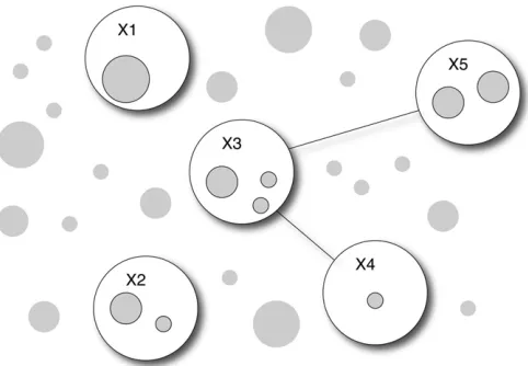
2. The method handles correlation among sets of SNPs via Bayesian graphical models, such that indirect disease asso-ciations purely due to correlation with“true”disease var-iants arefiltered out. Unlike typical solutions that model the dependence structure of all variables, our approach handles dependence implicitly and locally. While the former is computationally prohibitive in GWAS, the lat-ter can satisfactorily resolve the dependence issue with drastically reduced computation time.

3. With dependence accounted for, the method pinpoints the most likely subsets of disease variants within local

regions, such that the method achieves much improved mapping resolution than existing tools.

4. The method handles both common and rare SNPs with-out arbitrary separation. We allow SNPs to be represented in both forms of a single unit (to test the effect of itself) and as part of a group of SNPs (to test its group effect jointly with other SNPs). More generally, the method is

flexible in that it allows the users to group SNPs with overlaps. Our method analyzes all SNP sets and their com-binations in a joint Bayesian probabilistic model, where the best SNP sets associated with the disease are automat-ically selected and the multiplicity issue is handled via Bayesian priors.

combinations of SNP sets to maximize the power of association mapping, and we learn the disease association structure via Bayesian graphs.

Our method evaluates the association between a SNP set and the disease traits using a Bayesian regression model. In a regression framework, covariates such as environmental factors, individual factors, and population structure components can be incorporated to account for confounding effects. Different from conventional regression models, our regression inversely models the distribution of genotype data on the disease traits. This inverse modeling has several advantages: (1) genotype distribution is relatively simple to model, whereas disease traits may follow any distribution; (2) direct associations with the disease can be effectively distinguished from indirect associations (due to SNP correlation) by explicitly modeling the joint distribution of genotypes at multiple SNPs; and (3) we can detect genetic effects on the variation or high-order moments of the disease traits by including interaction terms, and we can also include multivariate traits.

Using data from the 1000 Genomes project (1000 Genomes Project Consortium 2010), we performed extensive simulation studies to evaluate the power of our method compared to six sets of existing rare variant methods (Pan 2009; Price et al. 2010; Nealeet al.2011; Wuet al.2011; Leeet al.2012; Ionita-Lazaet al.2013) and a single SNP test method (Conneely and Boehnke 2007). We show that the new method performs simi-larly to the best rare variant methods when testing only a handful number of very rare variants. The method, however, performs better and sometimes substantially so, when moderately rare or common variants are included and/or when the disease variants are not randomly distributed in a predefined genomic interval for testing. In addition, when testing associations in a large collection of variants, which is the common scenario in practice, our method substantially outperforms existing methods. Beyond set-based tests, the new method further reveals the locations of the most likely disease variants via Bayesian variable selection. We demonstrate an application of our method to a whole-genome resequencing data set generated in our laboratory from 97 type 1 diabetes (T1D) patients, where we handled sample stratifi ca-tions and identified novel T1D loci.

Materials and Methods

The general model framework

LetY =(Y1,. . .,Yp) denote the disease data measured onp

traits, whereYjforj= 1,. . .,pis an-dim vector containing

data innindividuals. Since we useYas independent variables, it may take any measurements such as discrete, continuous, and categorical. LetX= (X1,. . .,XL) denote the genotype data

atLSNP sets (each SNP set may contain one or more SNPs; i.e., eachXicould be a matrix by itself), andZ= (Z1,. . .,Zm) denote additionalmcovariates to be adjusted for their confound-ing effects. Again, eachXl(l= 1,. ..,L) andZk (k= 1,...,m)

contain data innindividuals. Our task is to identify a subset of SNPs inXthat are directly associated (not due to LD with other

genotyped SNPs) with at least one trait inY, conditioning onZ. LetXAandXUdenote a nonoverlapping partition of SNPs, such

thatXAinclude the SNPs directly associated withY,XUdenote

the remaining SNPs, andX= {XA,XU}. LetAdenote the

par-tition. We write the joint probability

Pr_ðX_;Y_;Z_;A_{Þ ¼}Pr_ðXUjXA;Y;Z;AÞPrðXAjY;Z;AÞPrðY;ZÞPrðAÞ

¼ Pr_ðXUjXA;Z;AÞPrðXAjY;Z;AÞPrðY;ZÞPrðAÞ:

(1)

The second equality in (1) is due to our definition thatXUis

not associated withYconditioning onXAandZ(butXUcould

be marginally associated withYdue to its LD withXA). This

is a major distinction between our method and existing ones, as the latter do not distinguish the two.

Our goal is to identify the partitionA, which relies solely on Pr(XU|XA, Z,A)Pr(XA|Y,Z,A)Pr(A), which can be rewritten as

PrðXUjXA;Z;AÞPrðXAjY;Z;AÞPrðAÞ

¼PrðXjZÞ½PrðAÞPrðXAjY;Z;AÞ=PrðXAjZ;AÞ: (2)

Note that Equation 2 is proportional to the odds ofXAagainst

Yconditioning onZ, along with a prior distribution of partition A. We droppedAfrom the condition of probability function Pr (X|Z) because the partition is irrelevant without disease infor-mationY. Therefore, we need only to compute the term within the brackets in (2) to identify the partitionA.

When the size ofAis large, directly modeling Pr(XA|Y,Z,A)

and Pr(XA|Z,A) as multivariate distributions can be

power-less due to the quickly increasing size of model parameters. Instead, we use undirected acyclic graphs (Zhang 2011) to reduce model complexities. LetGA= (NA,EA) andGA9= (NA9,

EA9) denote the graphical structures ofXAwith and withoutY,

respectively, where a node (N) denotes one or a set of SNPs in XA, and an edge (E) denotes“interactions”(joint association)

between the two nodes. We augment Pr(XA|Y,Z,A) in (2) to

PrðGA;XAjY;Z;AÞ ¼PrðGAÞPrðXAjGA;Y;Z;AÞ ¼PrðGAÞ

Y

a in NAPrðXajGA;Y;ZÞ

Y

aa9 in EA PrXaþa9GA;Y;Z

.

½PrðXajGA;Y;ZÞPrðXa9jGA;Y;ZÞ; (3)

where“ainNA”denotes the enumeration of all nodes, and

aa9inEAdenotes the enumeration of all edges. Similarly,

we write Pr(XA|Z,A) in (2) as

PrðXAjZ;AÞ ¼

X

G9

A

PrG9_APrXAjG9A;Z;A

: (4)

The difference between (3) and (4) is that the graphs are different, and we sum overG9A in (4) as it is in the

denom-inator of the odds in (2). Plugging (3) and (4) back into (2) [replace Pr(XA|Y,Z,A) in (2) by Pr(GA,XA|Y,Z,A) in (3)], we

use MCMC to learn the SNP partitionAas well as the graph GA, which we call a disease graph that further details the

the size ofAis Binomial(L,p). We use a Pitman–Yor process (Pitman and Yor 1997) to further partition SNP sets in XA

into nodes inGA(andGA9), with strength parameter 0.5. We

use independent Bernoulli priors with probability 0.5 to in-dicate the presence of an edge between each pair of nodes, with constraint that the graph must be acyclic (for simplicity, we ignore the difference in normalizing constants due to this constraint, and such omission can be regarded as part of a prior setup).

From (2), the model parameters to be updated by MCMC include the SNP partitionAand the disease graphGA(nodes

and edges). We show in the next section that additional param-eters for modeling the data distribution can be analytically in-tegrated out. As a result, after random initialization, our MCMC algorithm works by iteratively adding/removing a SNP set in/ out ofXA one at a time and, simultaneously, updatingGA by

adding/removing a SNP set in/out of a graph node and adding/ removing an edge between two nodes. All these updating pro-cedures are done via standard Gibbs samplers derived from (2), details of which are omitted here but can be found in Zhang (2011). Finally, enumerating all graphs in (4) can be time con-suming for large size ofA. For quick computation, we provide the users with an option to enumerate only a subset of graphs G9Athat shares the same structure as that ofGAexcept for the

current SNP set to be updated;i.e., we enumerate only {G9A:

G9A;2i= GA,-i} in (4), where SNP setiis the set to be added/

removed fromXA. This is an approximate solution that does not

yield the correct posterior distribution from (2). Empirically, however, we found that this option produces very similar results to that produced by the full model when the signals are not extremely strong (as is the case in GWAS), but it results in a dramatic reduction in computing time (Zhang 2011).

The rationale underlying our approach is to evaluate whether a SNP seti(Xi) should be added into the disease

partitionA, given those SNP sets already included inAand the covariatesZ. This is done by comparing probabilities (3) and (4) forXi_during MCMC, where (3) represents the probability

thatXiis associated withYconditioning on currentXAandZ, and

(4) represents not associated. Note that (3) is a more complex model (with more parameters) than (4) due toY. Via Bayesian priors, therefore, (3) tends to be smaller than (4) whenXiis not

associated withY, and thusXitends not to be included in the

disease partitionA. Also note that SNP dependence is modeled via Bayesian graphical models in (4), which accounts for LD. As a result, our method is able to distinguish direct disease associ-ation from indirect associassoci-ation due to SNP correlassoci-ation.

Bayesian regression for a set of variants

A major difference between the new method and the original BEAM3 algorithm lies in the definition of the probability functions Pr(Xa|GA,Y,Z,A) in (3) and Pr(Xa|GA,Z,A) in (4).

In BEAM3, we used a saturated multinomial distribution to describe the genotypes in SNP setXa, which works powerfully

for common SNPs, but not so much for rare variants because there are many more rare variants to be tested together. It is also analytically complicated to incorporate continuous values

ofYand covariatesZin a multinomial distribution. In the new method, therefore, we model Pr(Xa|GA,Y,Z,A) and Pr

(Xa|GA,Z,A) by a multivariate regular Bayesian regression

function. Using conjugate priors, it is analytically easy to compute and straightforward to incorporate any forms of disease traits Y and covariates Z without model parameter estimation.

LetXadenote a (n3q) response matrix of genotype data,

wherendenotes the total number of individuals andqdenotes the number of SNPs to be tested in a set. By default,Xa

con-tains the minor allele counts (0, 1, 2) per individual per SNP. Alternatively, a dummy coding for the three genotypes can be used. LetYbe a (n3p) predictor matrix of disease traits. LetZ be a (n3m) matrix of covariates. Without loss of generality, we assume that Xa, Y, and Z are all column centered. Our

regression model assumes that

Xa N ðYBþZC; SÞ;

whereBdenotes a (p3q) matrix representing the effects ofY on SNPs inXa,Cdenotes a (m3q) matrix representing the

effects of covariates, and S denotes a (q 3 q) covariance matrix of noise.

Since our interest is only to identify SNP partitions, whereas SNP effects can always be estimated in postanalysis, we analytically integrate out the parameters (B,C,S). We assume thatBfollows a matrix normal distribution MN(0,HB,

S),C follows another matrix normal distribution MN(0,HC,

S), andSfollows an inverse Wishart distribution IW(C,n). Here,HB= diag(c/q,q),HC=diag(h,m),C=Ιq,n=u/2+1

denotefixed hyperparameters. By default, we choosec= 0.01 andh= 1000. A small value ofcpenalizes on large magnitude of the effects of disease Y, and a large value ofhallows any magnitude of the effects of covariatesZ.

LetH= diag(HB,HC) denote a (p + m)3(p + m) diagonal

block matrix carryingHBandHCalong its diagonal,U= (Y,Z)

denote an3(p + m) matrix withYandZcombined. Following standard procedures, it is straightforward to show the following conditional probability function with model parameters (except for hyperparameters) integrated out

Pr_ðXajGA;Y;ZÞ ¼

1

pnq=2_IpþmþHU9Uq=2 Gq

½qþn=2 þ1 IqþLðqþnÞ=2þ1Gqðq=2þ1Þ

where L¼X_a9

In2U

H21þU9U21U9

Xa;

(5)

whereGq(.) denotes a multivariate Gamma function.

Using (5), we can further obtain the null function Pr(Xa|GA,

Z) by removingYfromUand modify the dimension parameters for matrices accordingly. Finally, we plug (5) back into (3) and (4), which completes the new model.

continuous parameters. The novelty of our method does not lie in Equation 5. Instead, it lies in our joint modeling approach defined in (2), the usage of Bayesian graphical models in (3) and (4) for implicit modeling of SNP correlation, and the Bayesian approach for integrating common and rare variants via a joint probabilistic framework for testing their marginal and joint effects. To our best knowledge, no other methods have been able to achieve the same goals and simultaneously being computationally feasible for large data sets.

Construction of SNP sets

When testing a single set of SNPs, Equation 5 can synergize information of the disease effects in both directions, which is similar to the existing variational methods. Our model further dynamically explores combinations of SNP sets for joint testing via MCMC. This is a variable selection procedure that is unique compared to hypothesis testing. When a pathway involves many genes, it is unclear whether it will be more powerful to test all genes in the pathway or to focus on a subset of genes. Using our method, the users can define each gene or a subset of genes as a variable and then let the method explore combinations of SNP sets for the most powerful association mapping. Each gene often carries several SNPs, both common and rare. It is unclear what is the best cutoff for“rare”variants to be tested together. In our method, the users can define a SNP as a variable by itself and simultaneously group the SNP with others as a set. Our method then automatically evaluates the individual effect and the group effect of the same SNP simultaneously to maximize power.

The new method allows three ways to define sets of SNPs ahead of the analysis:

1. As used by current rare variant methods, the users can define SNP sets in genic regions based on biological knowledge.

2. The users can input two cutoffsa1#a2and a parameter dto define SNP sets, particularly for intergenic regions. For SNPs whose MAF.a1, we define the SNP as a vari-able by itself. For SNPs whose MAF,a2, we group them together if they are within dSNPs away. Since a1#a2, SNPs with MAF betweena1anda2will be evaluated for both single and group effects. This approach creates a buffer that effectively alleviates the need for a hard andad hocthreshold for defining common and rare var-iants. To the extremes, whena1=a2= 0, all SNPs will be tested individually; whena1=a2= 1, all SNPs will be tested in sets; and whena1= 0,a2= 1, all SNPs will be tested for both individual and group effects. By default, we leta1= 0.005,a2= 0.05,d= 30.

3. The users can ask the method to hierarchically split large SNP sets into smaller sets. For a predefined SNP set con-taining many SNPs, we introducek additional SNP sets that are subsets of the original SNP set. If some of thek new SNP sets still contain too many SNPs (greater than a user-specified threshold), we split them further. As a re-sult, the sets of SNPs to be analyzed will include (i) the

original large SNP set; (ii) theksubsets; and (iii) addi-tional smaller subsets split hierarchically. This creates new SNP sets in different sizes to be tested for associa-tion, which increase the chance for the true disease var-iants to be properly covered and detected with improved power.

In summary, our method allows for greater flexibility than existing methods in defining SNP sets, testing combi-nation of SNP sets, evaluating both individual and group effects, and testing both common and rare variants without hard cutoffs. Also, SNP sets may overlap, where the correla-tion among overlapping SNP sets is accounted for via probabilities.

Data simulation

We used the phased haplotype data from the 1000 Genomes project to generate simulated case control data sets in this study. Using individuals with European origins, we gener-ated new haplotypes as mosaic combinations of the 1000 Genomes haplotypes, with recombination rate 1 per 100 kb. We then generated new individuals by randomly pairing the new haplotypes. The data of each new individual contained genotypes at Lconsecutive SNPs in a randomly chosen re-gion. Among the LSNPs, we randomly selectedx SNPs as the disease variants. For a given disease model specified in Results, we then generated cases and controls from the new individuals according to the genotypes at thexselected SNPs.

Results

Simulation study in small data sets

Wefirst performed simulation studies to evaluate the power of our method (implemented in BEAM3) compared to seven categories of existing methods on SNP sets that are small enough (a few hundreds of SNPs) such that a single test can be performed on all SNPs together. The methods we compared with include (1) SKAT (Wuet al.2011), SKAT-O (Lee et al. 2012), and SKAT-C (Ionita-Laza et al. 2013), which are kernel regression methods, and SKAT-C combines effects of both rare and common variants; (2) MultiVar, a standard multivariate score test (Wald test); (3) SSU and SSUw (Pan 2009), unweighted and weighted sum of squared scores; (4) Common, a standard regression assum-ing same effect of all variants; (5) Sassum-ingle, a sassum-ingle SNP test reporting minimumP-value adjusted by multiple testing cor-rections (Conneely and Boehnke 2007); (6) C-alpha (Neale et al.2011), a homogeneity test of a set of Binomial propor-tions; and (7) VT1-4 (Priceet al.2010), a regression method subject to variable allele-frequency thresholds using four different criteria. These methods employ very different approaches and are good representatives of the current rare variant mapping algorithms. All methods are capable of detecting effects in opposite directions.

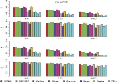
at 300 SNPs. Among the 300 SNPs, 15 (5%) are selected as disease variants. All models assume additive effects of the disease variants, and the effect size of each disease variant is given byl=p20.1747_{21 (Wuet al.2011), wherepdenotes} the MAF of the disease variant. Forp= 0.3, 0.03, and 0.003, the effect size is 0.23, 0.84, 1.76, respectively, which mimic the effect sizes observed in genome-wide association studies for complex diseases. The four disease models differ by the locations of disease variants and the directions of effects. In model 1 and model 2, we assume a uniform distribution of disease variants among the 300 SNPs, while in model 3 and model 4 we assume a clustered distribution. That is, in model 3 and model 4, the 15 disease variants are distributed within two nonoverlapping SNP clusters. Each cluster contains 30 SNPs, carrying 25% disease variants each, yet the overall percentage of disease variants among the 300 SNPs is still 5%. For the directions of effects, in models 1 and 3, we assumed independent and random directions of effects with probability 0.5 each, while in models 2 and 4, we assumed that all disease variants have positive effects to the disease risk.

To evaluate how each method performs with respect to the rareness of variants, the MAFs of the 300 SNPs in each data set was bounded above by 0.01, 0.05, and 0.5, respectively, representing very rare, moderately rare, and common + rare data sets. In the 1000 Genomes data, there are 33% SNPs in each category of MAF,0.01, between (0.01, 0.05), and.0.05, respectively. For each MAF bound and for each disease model, we simulated 1000 data sets to evaluate power. To control type I error rate, we did not use theP-values provided by the original methods, because the P-values provided by C-alpha and VT were seriously inflated, and the asymptoticP-values of MultiVar were too conserva-tive. Instead, we ran 200,000 permutations in each scenario to obtain empiricalP-values of all methods. For BEAM3, we set a1 = 0.005 anda2 = 0.05, such that SNPs with MAF

.0.005 forms its own SNP set, and SNPs with MAF,0.05 form groups with other SNPs within d= 15 SNPs. The test statistic for BEAM3 is the sum of posterior probabilities of disease association over all SNP sets in each data set, and P-value is calculated by comparing with the statistics obtained from permuted data.

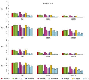
Figure 2 shows the power comparison of all methods on data sets with maximum MAF 0.01. In these data sets, only the very rare variants are included. We observed that SKAT, SSU and Calpha all performed similarly with the best power in all scenarios. Our method (BEAM3), in comparison, achieved similar power in most cases. Overall, models 2 and 4 with all positive effects are detected by all methods more easily than by models 1 and 3 with opposite effects. The multivariate regression score test (MultiVar) performed the worst in all scenarios, whereas the common effect method (Common) performed poorly for models 1 and 3, because the effects were in opposite directions. The variable threshold approach (VT) performed poorly too; particularly, its power was worse than the single SNP test (Single) in all scenarios.

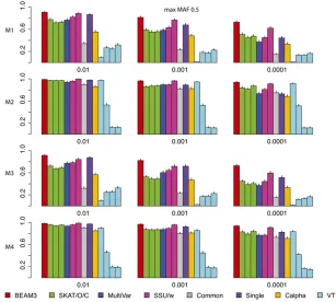
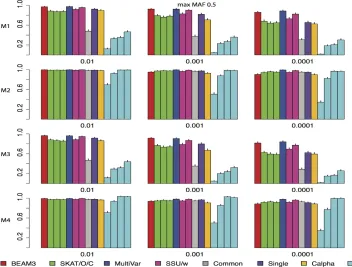
Figure 3 and Figure 4 show the power comparisons on data sets with maximum MAF 0.05 and 0.5, respectively, which included not only very rare variants, but also moder-ately rare and common variants, respectively. It is seen that the powers of all methods increased as more common variants were included. For all models and at all significant levels, BEAM3 performed consistently and sometimes substantially better than the others. Again, SKAT, SSU, and Calpha performed similarly in all scenarios, and they obtained better power than the remaining methods in most cases. It is worth mentioning that, apart from Single, our method is the only approach that can reveal the locations of disease variants within each data set. We have also performed additional simulation studies with each data set carrying 30% disease variants, for which we observed similar results (supporting informationFile S1). In summary, our method performed similarly or better than existing methods when testing on a small set of SNPs, particularly when moder-ately rare and common SNPs were included. Even for the very rare SNPs, our method still performed competitively to the best methods, but we further pinpointed disease variants within each set.

Simulation study in large data sets

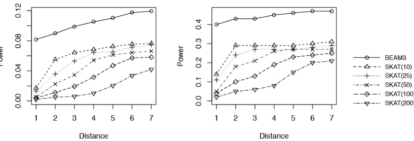
We next evaluated the power of our method on larger data sets containing 1000 cases and 1000 controls at 10,000 SNPs with maximum MAF ,0.05. In this case, no existing methods can perform a single test on all SNPs simulta-neously, but they have to split the SNPs into subsets and perform multiple tests. Based on the small data results, we compared only our method with SKAT, because SKAT per-formed similarly to SSU and C-alpha and was one of the best among all methods. In each data set, we simulated 50 dis-ease variants equally partitioned into 5 groups (10 disdis-ease variants per group). The disease variants in each group were randomly distributed within either a 5- or a 50-kb region, with equal probability. Also, the disease variants in a group either have 50% opposite directions of effects or have pos-itive effects, with 50% chance each. The effect sizes were determined in the same way as before. Since we cannot run SKAT to test all SNPs together, we partitioned each data set into equal-sized windows containing M SNPs per window and we ran SKAT in each window separately. We tested SKAT for M = 10, 25, 50, 100, 200, respectively. We ran our method on the entire data set with a1= 0.005, a2= 0.05, and d = 30 (number of SNPs per set for those with MAF,a2). We also used the hierarchical splitting strategy to split each 30-SNP set intok= 4 subsets and kept both for analysis. Again, we used permutationP-value to control type I errors. For SKAT, the P-value from each MSNP window was used as the statistic to obtain data-wide significance thresholds. For BEAM3, the posterior probability of disease association from each predefined SNP set was used as the statistic to obtain data-wide significance thresholds.

To calculate power, wefirst identified the significant SNP sets reported by each method at data-wide significance level 0.01. For each significant SNP set, we then identified its nearest true disease variant to the center of the SNP set. The disease variant (or the region it belonged to) was counted as detected if the distance (in number of SNPs) between the two was within a threshold.

Figure 5 shows the results obtained from 100 simulated data sets of 10,000 SNPs each (MAF,0.05). We observed that BEAM3 performed considerably and consistently better in terms of detecting and localizing disease variants and disease regions, compared to SKAT using any window size. The performance of SKAT varied considerably for different window sizes. Additional simulation studies of even larger Figure 2 Comparison on data sets with MAF bounded at 0.01.x: significance.y: power for four models.

data sets containing 100,000 SNPs showed similar results (supporting information,File S1). In practice, the best win-dow size is never known for hypothesis-testing methods. It is likely that both rare and common variants affect the disease risks, either independently or jointly. Aflexible method like ours is thus strongly desirable.

Type 1 diabetes resequencing data

We applied BEAM3 to a whole-genome resequencing (WGS) data generated in our laboratory on blood-derived DNA from 97 T1D patients. The samples were processed using SOLiD5500 sequencers. For sequence alignment, variant calling, and annotation, we employed our parallel read mapping and variant-calling pipeline, using Burrow Wheeler alignment (BWA) (Li and Durbin 2009, 2010), BOWTIE (Langmead et al. 2009), and SAMtools (Li et al. 2009) to call SNVs and indels. The output is in sequence alignment/ mapping (SAM) format we compressed into a binary format (BAM). The BAMfiles that passed quality control (QC), in-cluding proportion of mappable reads and number of unique start sites, were subsequently used for downstream analysis. The average number of reads for the WGS data were 6–83 (i.e., low coverage) of high-quality sequence data following standard QC procedures.

Because no controls are sequenced in this study, we downloaded 85 unrelated CEU samples, whose origins are the closest to the T1D patients in this study, from the 1000 Genomes project. We retained only the SNPs that appeared in both the T1D samples and the CEU controls. We removed SNPs with.10% missing values and those with significant Hardy–Weinberg disequilibrium (P-value,1026_{). We imputed}

missing genotypes by sampling within each SNP and we removed nonpolymorphic SNPs. Thefinal data set contained 97 cases and 85 controls at 2.93 million SNPs.

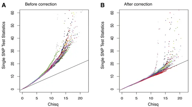
Since the cases and controls are generated by different protocols, we observed sample stratification. As shown in Figure 6A, single SNP test statistics are inflated genome-wide. We therefore decorrelated samples as follows: (1) we calculated a covariance matrix Vof the 182 individuals using SNPs whose absolute correlation with the disease status is ,99 percentile; (2) we decomposed V =LL9by Cholesky decomposition; and (3) we calculated new “ geno-types”byXnew=X(L9)-1. As a result, the new“genotypes”are decorrelated under Normality assumption. Figure 6B shows that the single SNP test statistics are “correct” after this adjustment.

After correcting for sample stratification, we ran our method witha1= 0.05,a2= 0.1,d = 30 with hierarchical splitting (k = 4). Due to computational constraints, we applied our method on each chromosome separately. We ran our method four times on each chromosome independently and then sum-marized the posterior probabilities of associations by averag-ing. We reported in Table 1 the top 12 detected T1D loci whose posterior probabilities were .0.25. Based on genome-wide permutations, our criteria yieldedP-value,1027_{. Among} the 12 detected loci, 7 had at least two SNPs within 500 kb showing single-SNP testP-value,1025_.

of HLA class I molecules and play important roles in regulation of the immune response. In addition, downregulation of KIRD3L1 has been shown to enhance inhibition of type 1 diabetes (Qin et al.2011). Second, the locus chr5:17.48–17.62 Mb is 200 kb downstream of gene BASP1. This gene has been reported to promote apoptosis in diabetic nephropathy (Sanchez-Nino et al. 2010), and defective apoptosis is known to play an important role in type 1 diabetes (Hayashi and Faustman 2003). Incidentally, two other loci (chr10:127.56–127.65 Mb, chr22:18.62–18.92 Mb) also overlapped with genes (FANK1, DHX32, USP18) that are related to cell apoptosis. While FANK1 and DHX32 regulate T-cell apoptosis (Alli et al.2007; Wanget al.2011), USP18 is a key regulator of the interferon-driven gene network modulating pancreatic beta cell

in-flammation and apoptosis (Santin et al.2012). Third, 3 (chr1:24.28–24.39 Mb, chr7:159.10–159.13 Mb; chr22:18.62– 18.92) out of the 12 loci either overlapped or were near genes (PNRC2, VIPR2, DGCR6, PRODH) associated with obesity and type 2 diabetes. PNRC2 is a nuclear receptor coactivator that regulates energy expenditure and adiposity in mice (Zhouet al. 2008), which are the keys to understand obesity, insulin re-sistance, and type 2 diabetes. VIPR2, DGCR6 and PRODH are known to be significantly associated with schizophrenia (Vacic et al.2011; Welshet al.2011; Liuet al.2002), a mental dis-order that is associated with decreased risk of type 1 diabetes (Juvonenet al.2007) and increased risk of type 2 diabetes (Schoepfet al.2012).

The human major histocompatibility complex (MHC) region is a well-known T1D locus. Our analysis did not capture this region at the genome-wide significance level due to several reasons. First, the sample size of our data set is small. The lead T1D SNP rs9268645 in MHC, reported by Barrettet al.(2009), has associationP-value,,1e-100 from a metaanalysis com-bining two independent studies carrying over 10 thousands of individuals. This SNP is captured in our study, with MAF 0.47 in cases and 0.40 in controls. These MAFs were statistically the same as those observed in WTCCC T1D data set (Wellcome Trust Case Control Consortium 2007) (0.46 in cases and 0.40 in controls, respectively), but has insignificantP-value (.0.1) due to the small sample size. Should the sample size be 10000 with the same MAFs, itsP-value will decrease to,1e-50. Sec-ond, there are many missing values due to low coverage sequencing. The lead T1D MHC SNP rs9273363 reported by Nejentsev et al. (2007) hadP-value 1e-298, yet it was removed from our study because of 38% missingness (no reads). Should this SNP be retained in our study, but simply ignoring the missing values, we will obtain case MAF 0.63, control MAF 0.33, andP-value 2.2e-7 before adjusting for sam-ple stratification. These MAFs are again similar to those ob-served in WTCCC T1D data set (case MAF 0.71, control MAF 0.30). Third, our data set has sample stratification problem due to lack of controls, which further reduces the power.

Given that we already know that MHC carries T1D variants, we applied our method to the MHC region Figure 5 Power comparison between BEAM3 and SKAT: (A) Power for detecting variants and (B) power for detect-ing regions. Distance: maximum allowed number of SNPs between the center of a reported significant SNP set (data-wideP-value 0.01) and the nearest true disease variant, such that the true variant is counted toward power. SKAT: in the parentheses shows the number of SNPs per set. o: BEAM3;D: SKAT(10); +: SKAT(25); x: SKAT(50);): SKAT(100);

=: SKAT(200)

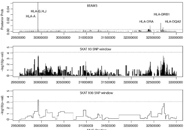
(chr6:29.5 Mb–33 Mb, hg19, 6472 SNPs) specifically to localize

“causative”T1D variants. The result is shown in Figure 7. Our method pinpointed four T1D loci with MHC-wide significance ,0.05, including locus 29922754 bp in genes HLA-H, HLA-G, HLA-J and at 10 kb downstream of HLA-A, locus 32417825– 32417891 bp at 3 kb downstream of HLA-DRA, locus 32651168– 32651254 bp at 17 kb upstream of HLA–DRB1, and locus 32705193–32705276 bp at 2 kb upstream of HLA–DQA2. The latter three loci are all within the well-known HLA–DR– DQ genes in MHC class II complex. For comparison, we also ran SKAT in the same MHC region using two different

win-dow sizes: 10 and 100 SNPs, respectively. As shown in Figure 7, SKAT detected the HLA–H,G,J locus, but failed to yield significantP-values at the HLA–DR–DQ region.

Discussion

In this article we introduced a powerful andflexible method for simultaneous testing of rare and common variants associated with complex diseases. Distinct from existing approaches, our method utilizes a joint statistical model to test all variants genome-wide simultaneously. The benefits are twofold: joint Table 1 Loci detected in the T1D resequencing data set

Detected locia

Assoc. prob.b

Multi-assoc.c _{Nearest genes}d

chr1:24281021–24388679 1.00 (1.00) Yes SRSF10, MYOM3,PNRC2 chr3:625496–705294 1.00 (1.00) Yes AK126307 (CNTN6)

chr4:190436494–190538640 0.82 (2.06) Yes (DUX2, DUX4L4, FRG2, FRG1, TUBB4Q) chr5:17479389–17622489 0.99 (0.99) No (LOC401177,BASP1, BC028204)

chr6:67706682–67780247 0.98 (0.98) No None, but has strong Pol2 signal in K562 and DNA methylation. chr7:159100528–159126143 0.66 (0.66) Yes (VIPR2)

chr9:68435907–68800509 1.00 (1.00) No LOC100132352, AK096159, LOC642236 chr10:127556783–127650870 0.85 (0.86) No FANK1,DHX32

chr16:70813237–71062992 0.29 (0.67) Yes HYDIN, VAC14

chr19:55268017–55332829 0.98 (0.98) Yes KIR2DL1-4,KIR3DL1,KIR2DL4,KIR2DS4 chr20:20109354–20184868 1.00 (1.00) No C20orf26 (CRNKL1)

chr21:14946923–15168502 0.43 (0.43) No POTED, DQ590589, DQ591735 (C21orf15, DQ586768) chr22:18622054–18923349 0.89 (1.14) Yes GGT3P,DGCR6,PRODH, AK302545, BC112340, BC051721,

AL117485, DQ786190, AK129567,USP18

a_{Positions are in hg19 coordinates.}

b_{Maximum posterior probability within the interval and the sum of posterior probabilities of all SNPs in the interval are in parentheses (italics}

indicate a significant difference between the two).

c_{Whether or not the interval carries more than one SNP with marginalP-value,10}25_.

d_{Genes overlap with the interval, and genes that do not overlap with the interval but are within the 500-kb neighborhood are in the parentheses.}

Genes in italic type are discussed in the main text.

associations or cumulative effects of multiple variants are detect-able with improved power by dynamic grouping of sets of variants; and our joint model accounts for correlation among variants, such that multiple disease variants within a local region can be detected and redundant associations due to LD arefiltered out. As a consequence, we are able to define sets of variants that overlap with each other without concerning about multicolinearity among variants. A variant may be simultaneously present in the data set as a single variant by itself and as groups of variants with others. The new method will then evaluate the effects of the variant both as a single variant and as groups, and one shows that the most power will be automatically detected. This feature significantly alleviated the burden on the users to define sets of variants to be tested, which is often arbitrary. At the same time, the users can still design their favorable sets of variants for joint testing based on their biological knowledge. While it is unclear how much effects of rare variants contribute to the complex diseases, it is most likely that both common and rare variants are contrib-uting to the disease risks to a different degree. We therefore believe that our method is more suitable to the current genome-wide association studies, where all genetic variants from sequencing studies are included in the analysis.

Our simulation studies have demonstrated the superior power of the new method compared to existing rare variant mapping tools. In the small data study, we observed that our method performed similarly to the best existing methods when testing only the very rare variants (MAF,0.01). When more common variants were included, our method achieved better power and sometimes substantially so. In the large data study, our method performed substantially better than existing meth-ods in terms of both power and mapping resolution. When applied to a whole-genome resequencing study of type 1 di-abetes, we handled sample stratification and detected novel loci that are biologically relevant to T1D. We further demonstrated afine mapping of T1D variants in the well-known MHC region, where we identified one locus in the HLA-G,H,J genes and three loci in the HLA–DR–DQ genes. In comparison, SKAT detected only one locus in MHC and its result is sensitive to window sizes. Many loci we detected involved common variants, which in part was due to the very limited sample size of the study, but also perhaps indicated that exclusively focusing on rare var-iants may not be the best strategy.

Our method can be directly applied to other types of data, such as copy-number variations and genomic/epigenetic data. In addition, our method can be used for QTL mapping, and covariates such as environmental factors can be included. Currently the method does not allow detection of SNP– environment interactions associated with the disease, but a simple modification can be added to allow detecting disease associated interactions between SNPs and covariates. The method can also take input of multiple traits simultaneously, such that SNPs asso-ciated with one or multiple disease traits can be detected. By inversely regressing SNPs on disease traits, we avoid modeling the distributions of disease traits. An interesting extension of the method is therefore to include kernels to detect nonlinear

associations between SNPs and multiple disease traits. The URLs for data presented herein are as follows:

1000 Genomes:http://www.1000genomes.org/

Online Mendelian Inheritance in Man (OMIM):http://www.ncbi. nlm.nih.gov/omim

BEAM3:http://stat.psu.edu/~yuzhang/software/beam3.tar

Source code of BEAM3 can be found in Supporting Informa-tion,File S2.

Acknowledgments

Y.Z. is supported by National Institutes of Health grant R01-HG004718.

Literature Cited

1000 Genomes Project Consortium, 2010 A map of human ge-nome variation from population-scale sequencing. Nature 467: 1061–1073.

Alli, Z., Y. Chen, S. A. Wajid, B. Al-Saud, and M. Abdelhaleem, 2007 A role for DHX32 in regulating T-cell apoptosis. Antican-cer Res. 27(1A): 373–377.

Barrett, J. C., D. G. Clayton, P. Concannon, B. Akolkar, J. D. Cooper et al., 2009 Genome-wide association study and meta-analysis_find that over 40 loci affect risk of type 1 diabetes. Nat. Genet. 41(6): 703_–707.

Basu, S., and W. Pan, 2011 Comparison of statistical tests for disease association with rare variants. Genet. Epidemiol. 35: 606–619.

Bodmer, W., and C. Bonilla, 2008 Common and rare variants in multifactorial susceptibility to common diseases. Nat. Genet. 40: 695–701.

Conneely, K. N., and M. Boehnke, 2007 So many correlated tests, so little time!: rapid adjustment of p values for multiple corre-lated tests. Am. J. Hum. Genet. 81: 1158–1168.

Han, F., and W. Pan, 2010 A data-adaptive sum test for disease association with multiple common or rare variants. Hum. Hered. 70: 42–54.

Hayashi, T., and D. L. Faustman, 2003 Role of defective apoptosis in type 1 diabetes and other autoimmune diseases. Recent Prog. Horm. Res. 58: 131–153.

Ionita-Laza, I., S. Lee, V. Makarov, J. D. Buxbaum, and X. Lin, 2013 Sequence kernel association tests for the combined effect of rare and common variants. Am. J. Hum. Genet. 92: 841_–53. Juvonen, H., A. Reunanen, J. Haukka, M. Muhonen, J. Suvisaari et al., 2007 Incidence of schizophrenia in a nationwide cohort of patients with type 1 diabetes mellitus. Arch. Gen. Psychiatry 64: 894–899.

Langmead, B., C. Trapnell, M. Pop, and S. L. Salzberg, 2009 Ultrafast and memory-efficient alignment of short DNA sequences to the human genome. Genome Biol. 10: R25. Lee, S., M. J. Emond, M. J. Bamshad, K. C. Barnes, M. J. Rieder

et al., 2012 Optimal unified approach for rare-variant associa-tion testing with applicaassocia-tion to small-sample case-control whole-exome sequencing studies. Am. J. Hum. Genet. 91: 224–237.

Li, B., and S. M. Leal, 2008 Methods for detecting associations with rare variants for common diseases: application to analysis of sequence data. Am. J. Hum. Genet. 83: 311–321.

Li, H., and R. Durbin, 2010 Fast and accurate long-read align-ment with Burrows–Wheeler transform. Bioinformatics 26: 589–595.

Li, H., B. Handsaker, A. Wysoker, T. Fennell, J. Ruan et al., 2009 The sequence alignment/map format and SAMtools. Bio-informatics 25(16): 2078–2079.

Lin, D. Y., and Z. Z. Tang, 2011 A general framework for detect-ing disease associations with rare variants in sequencdetect-ing studies. Am. J. Hum. Genet. 89: 354–367.

Liu, H., S. C. Heath, C. Sobin, J. L. Roos, B. L. Galke et al., 2002 Genetic variation at the 22q11 PRODH2/DGCR6 locus presents an unusual pattern and increases susceptibility to schizophrenia. Proc. Natl. Acad. Sci. USA 99: 3717_–3722. Madsen, B. E., and S. R. Browning, 2009 A groupwise association

test for rare mutations using a weighted sum statistic. PLoS Genet. 5: e1000384.

Morgenthaler, S., and W. G. Thilly, 2007 A strategy to discover genes that carry multi-allelic or mono-allelic risk for common diseases: a cohort allelic sums test (CAST). Mutat. Res. 615: 28– 56.

Morris, A. P., and E. Zeggini, 2010 An evaluation of statistical approaches to rare variant analysis in genetic association stud-ies. Genet. Epidemiol. 34: 188–193.

Neale, B. M., M. A. Rivas, B. F. Voight, D. Altshuler, B. Devlinet al., 2011 Testing for an unusual distribution of rare variants. PLoS Genet. 7: e1001322.

Nejentsev, S., J. M. Howson, N. M. Walker, J. Szeszko, S. F. Field et al., 2007 Localization of type 1 diabetes susceptibility to the MHC class I genes HLA-B and HLA-A. Nature 450(7171): 887– 892.

Pan, W., 2009 Asymptotic tests of association with multiple SNPs in linkage disequilibrium. Genet. Epi. 33: 497_–507.

Pitman, J., and M. Yor, 1997 The two-parameter Poisson–Dirichlet distribution derived from a stable subordinator. Ann. Probab. 25: 855–900.

Price, A. L., G.V. Kryukov, P. I. W. de Bakker, S. M. Purcell, and J. Stapleset al., 2010 Pooled association tests for rare variants in exon-resequencing studies. Am. J. Hum. Genet. 86: 832–838. Qin, H., Z. Wang, W. Du, W. H. Lee, X. Wuet al., 2011 Killer cell

Ig-like receptor (KIR) 3DL1 down-regulation enhances inhibi-tion of type 1 diabetes by autoantigen-specific regulatory T cells. Proc. Natl. Acad. Sci. USA 108: 2016–2021.

Sanchez-Niño, M. D., A. B. Sanz, C. Lorz, A. Gnirke, M. P. Rastaldi et al., 2010 BASP1 promotes apoptosis in diabetic nephropa-thy. J. Am. Soc. Nephrol. 21: 610–621.

Santin, I., F. Moore, F. A. Grieco, P. Marchetti, C. Brancoliniet al., 2012 USP18 is a key regulator of the interferon-driven gene network modulating pancreatic beta cell inflammation and ap-optosis. Cell Death Dis. 3: e419.

Schoepf, D., R. Potluri, H. Uppal, A. Natalwala, P. Narendranet al., 2012 Type-2 diabetes mellitus in schizophrenia: increased prevalence and major risk factor of excess mortality in a natural-istic 7-year follow-up. Eur. Psychiatry 27: 33–42.

Schork, N. J., S. S. Murray, K. A. Frazer, and E. J. Topol, 2009 Commonvs.rare allele hypotheses for complex diseases. Curr. Opin. Genet. Dev. 19: 212–219.

Shendure, J., and H. Ji, 2008 Next-generation DNA sequencing. Nat. Biotechnol. 26: 1135–1145.

Vacic, V., S. McCarthy, D. Malhotra, F. Murray, H. H. Chouet al., 2011 Duplications of the neuropeptide receptor gene VIPR2 confer significant risk for schizophrenia. Nature 471: 499–503. Wang, H., W. Song, T. Hu, N. Zhang, S. Miaoet al., 2011 Fank1 interacts with Jab1 and regulates cell apoptosis via the AP-1 pathway. Cell. Mol. Life Sci. 68: 2129–2139.

Wellcome Trust Case Control Consortium, 2007 Genome-wide association study of 14,000 cases of seven common diseases and 3,000 shared controls. Nature 447: 661–78.

Welsh, D. K., D. Craig, J. R. Kelsoe, E. S. Gershon, S. M. Lealet al., 2011 Duplications of the neuropeptide receptor gene VIPR2 confer significant risk for schizophrenia. Nature 471: 499–503. Wu, M. C., S. Lee, T. Cai, Y. Li, M. Boehnke et al., 2011 Rare-variant association testing for sequencing data with the se-quence kernel association test. Am. J. Hum. Genet. 89: 82–93. Zawistowski, M., S. Gopalakrishnan, J. Ding, Y. Li, S. Grimmet al., 2010 Extending rare-variant testing strategies: analysis of noncoding sequence and imputed genotypes. Am. J. Hum. Genet. 87: 604_–617.

Zhang, Y., 2011 A novel Bayesian graphical model for genome-wide multi-SNP association mapping. Genet. Epi. 36: 36_–37. Zhou, D., R. Shen, J. J. Ye, Y. Li, W. Tsark et al., 2008 Nuclear

Receptor Coactivator PNRC2 Regulates Energy Expenditure and Adiposity. J. Biol. Chem. 283: 541_–553.

GENETICS

Supporting Information

http://www.genetics.org/lookup/suppl/doi:10.1534/genetics.114.167403/-/DC1

Dynamic Bayesian Testing of Sets of Variants in

Complex Diseases

Yu Zhang, Soumitra Ghosh, and Hakon Hakonarson

Appendix: Dynamic Bayesian Testing of Sets of Variants in Complex Diseases

Authors: Yu Zhang, Soumitra Ghosh, Hakon Hakonarson

Additional Power Comparison Results

Datasets are generated in the same way as described in the main text, except that each dataset

only contains 50 SNPs, such that there are 30% disease variants in each dataset. Figure S1-S3

show the power of our method compared to existing methods with maximum MAF bounded at

0.01, 0.05, and 0.5, respectively. Figure S4 shows the power comparison between BEAM3 and

SKAT on simulated datasets of 100,000 SNPs containing 100 disease variants.

 

Figure S1. Comparison on datasets with 30% disease variants and MAF bounded at 0.01

on 4 disease models. x: significance. y: power for 4 models.

 

Figure S2. Comparison on datasets with 30% disease variants and MAF bounded at

0.05 on 4 disease models. x: significance. y: power for 4 models.

 

Figure S3. Comparison on datasets with 30% disease variants and MAF bounded at 0.5 on

File S2 

Source code of BEAM3