HIGHLIGHTED ARTICLE
| GENETICS OF SEX
An Association Mapping Framework To Account for
Potential Sex Difference in Genetic Architectures
Eun Yong Kang,*,1Cue Hyunkyu Lee,†,‡,§,1Nicholas A. Furlotte,* Jong Wha J. Joo,** Emrah Kostem,*
Noah Zaitlen,††Eleazar Eskin,*,‡‡,2and Buhm Han†,‡,§,2
*Department of Computer Science and‡‡Department of Human Genetics, University of California, Los Angeles, California 90095, †Department of Medicine, Seoul National University College of Medicine, Seoul 03080, Republic of Korea,‡Department of Convergence Medicine, University of Ulsan College of Medicine, Seoul 05505, Republic of Korea,§Asan Institute for Life Sciences, Asan Medical Center, Seoul 05505, Republic of Korea,**Department of Computer Science and Engineering, Dongguk University-Seoul, Seoul 04620, Republic of Korea,††Department of Medicine, University of California, San Francisco, California 94143 ORCID IDs: 0000-0002-4482-5640 (C.H.L.); 0000-0002-2266-5164 (B.H.)
ABSTRACTOver the past few years, genome-wide association studies have identified many trait-associated loci that have different effects on females and males, which increased attention to the genetic architecture differences between the sexes. The between-sex differences in genetic architectures can cause a variety of phenomena such as differences in the effect sizes at trait-associated loci, differences in the magnitudes of polygenic background effects, and differences in the phenotypic variances. However, current association testing approaches for dealing with sex, such as including sex as a covariate, cannot fully account for these phenomena and can be suboptimal in statistical power. We present a novel association mapping framework, MetaSex, that can comprehensively account for the genetic architecture differences between the sexes. Through simulations and applications to real data, we show that our framework has superior performance than previous approaches in association mapping.
KEYWORDSAssociation Mapping; Genome-Wide Association Study; Genetics of Sex; Linear Mixed Model; Meta-Analysis
G
ENOME-WIDE association studies (GWAS) have success-fully identified numerous genetic loci associated with complex human traits. In recent years, increasing attention has been paid to the sex difference in genetic architectures in GWAS. A number of studies have found differences in effect sizes between males and females on loci associated with traits (Magiet al.2010; Boraskaet al.2012; Foxet al.2012; Kostis et al.2012; Mason and Lehert 2012; Chenet al.2013; Kubo et al.2013; Peterset al.2013; Porcuet al.2013; Randallet al. 2013; Kanget al.2014; Ohmenet al.2014). In particular, a meta-analysis of 46 studies of anthropomorphic phenotypes discovered seven loci with different effects between the sexes (Randall et al. 2013). Recently, Winkler et al.per-formed a meta-analysis of 114 studies on the waist/hip ratio adjusted for body mass index (BMI) to discover 44 loci showing significant sex-specific effects. Of these, 11 loci showed opposite effects between the sexes (Winkleret al.2015).
It remains unclear how best to account for the sex differ-ence in genetic architectures in association mapping. One traditional approach is to analyze each sex separately using sex-specific tests (SSTs). This approach is optimal for detect-ing sex-specific effects that only exist in one sex, but is not powerful for detecting effects that exist in both sexes. Another traditional approach is to analyze the whole sample and use sex as a covariate (CV). This approach is optimal for detecting effects that exist in both sexes in a constant effect size, but is not powerful for detecting sex-interacting effects that exist in both sexes in differing effect sizes.
In the present study, we first enumerate three possible phenomena that can be caused by the sex difference in genetic architectures. One is the effect size difference between the sexes at the associated locus, which was observed in previous studies (Randallet al.2013; Winkleret al.2015). Another is the effect size difference between the sexes at numerous loci spread throughout the genome with small effects, which can
Copyright © 2018 by the Genetics Society of America doi:https://doi.org/10.1534/genetics.117.300501
Manuscript received November 10, 2017; accepted for publication April 12, 2018; published Early Online May 11, 2018.
Supplemental material available at Figshare: https://doi.org/10.25386/genetics. 6071567.
1These authors contributed equally to this work.
2Corresponding authors: Department of Computer Science and Human Genetics,
be manifested as the polygenic background effects that in-teract with sex. Thefinal one is the phenotypic variance dif-ference between the sexes, which can be caused by many factors such as sex acting as a biological environment (e.g., hormone difference) and sex interacting with external envi-ronments (e.g., lifestyle difference). We show that these phe-nomena can often be observed in human traits collected in the North Finland Birth Cohort (NFBC) dataset (Sabattiet al. 2009).
Here, we present a novel association mapping framework, MetaSex, that can account for the potential sex difference in genetic architectures. Our framework comprehensively deals with the three aforementioned phenomena by uniquely com-bining linear mixed model and meta-analysis. Our linear mixed model includesfive variance components, where three components capture sex-interacting polygenic effects and two components capture sex-interacting variances. We then com-bine the observed effect sizes of the two sexes using the random effects model meta-analysis (RE) (Han and Eskin 2011) that provides high power for detecting sex-interacting effects. This whole procedure can be computationally chal-lenging because the five variance component model is im-practically slow to apply to millions of markers in GWAS. Therefore, we propose an approximated model that splits the five variance component model into two sex-specific models, each including only two variance components. Using simulations and real data, we demonstrate that our frame-work can powerfully detect associations in a wide range of situations.
Materials and Methods
MetaSex
Overview: We first provide an overview of our proposed framework. We constructed a toy example with six individuals (three females and three males). The equation in Figure 1A shows the components in our model for testing a single SNP. In this equation, vector y is the observed phenotype measure-ments, where subscriptsðfÞandðmÞdenote females and males.
m denotes the phenotypic mean.his the sex status indicator (female = 1 and male = 0), which is included as a CV to account for the sex-specific phenotypic mean. Thefirst column ofXis the genotype vector of the SNP, whose effect size isb. The second column of X is the genotype-by-sex interaction term (SNP 3 h), whose effect size isbg3s:ug is a variance
component that models the polygenic background effects from the genome-wide loci that affect both sexes. Consistent with the standard linear mixed model (Kanget al.2008, 2010; Zhou and Stephens 2012), we assume that ug follows a normal distribution with mean zero and variance-covariance matrix
s2
gK, whereKis the kinship matrix representing the
relation-ship between individuals.uf is an additional variance compo-nent that we introduce, which represents the female-specific polygenic effects. We assume thatuf has mean zero and var-iances2
g;fðK∘hh
TÞwhere∘indicates element-wise multiplication.
Similarly,umis a variance component representing the ma-le-specific polygenic effects, which has mean zero and var-iance s2
g;mðK∘ð12hÞð12hÞ
TÞ:
We then model separate error terms for females and males, assuming that error var-iances can be different.efis a female-specific error term that follows a normal distribution with mean zero and variance
s2 e;fðI∘hh
TÞ;
whereIis an identity matrix. Similarly,emis a male-specific error term that has mean zero and variance
s2
e;mðI∘ð12hÞð12hÞTÞ:
Applying this full model to GWAS can be computationally challenging because there arefive variance components tofit (ug; uf; um; ef; andem). Currently available linear mixed model methods for association mapping are optimized for models with two variance components (Kang et al. 2008, 2010; Zhou and Stephens 2012). If there is a third compo-nent, a state-of-the-art method uses a simple grid search (Lippertet al.2011). Thus,fittingfive variance components may require a three-dimensional grid search, which can be prohibitively slow for GWAS.
To expedite the application of our model to GWAS, we propose an efficient decomposition of the model. Suppose that we restrict our scope to individuals of one sex. Then, the full model withfive variance components collapses into a sex-specific model with two variance components (Figure 1B). Thus, the model can be efficiently solved using exist-ing approaches (Kang et al. 2008, 2010; Zhou and Ste-phens 2012). In the decomposed model, we cannot distinguish the whole-sample polygenic component (s2
g)
from the sex-specific polygenic components (s2 g;f ors
2 g;m)
because they follow exactly the same distribution condi-tioned on one sex. However, this distinction is unimportant for association mapping, because we want to control for both.
Finally, given the sex-specific effect size estimates and the standard errors [bcm;SEðbcmÞ;b
b
fSEðbb
fÞ], we apply a series ofstatistical tests. We first apply SST, which is optimal for detecting sex-specific effects. Then, to effectively detect sex-interacting effects, we combine the two sex-specific es-timates using the RE (Han and Eskin 2011) (Figure 1C), which explicitly models heterogeneity. As a result, our framework involves three tests (female SST, male SST, and RE), requiring multiple testing correction. A powerful multiple testing strategy can be to adjust the significance threshold for each test to maximize power while controlling for overall false positive rate (Eskin 2008). We identify and propose a set of thresholds for the three tests, what we call smart thresholding, that exactly controls the false positive rate to the GWAS threshold (531028) while maximizing
power.
Linear mixed model:Our MetaSex framework is based on a linear mixed model designed to account for the sex difference in genetic architectures. The standard linear mixed model to account for the polygenic background effects is:
whereyis a phenotype vector,mis an intercept,1is a vector of ones, x is a genotype vector, b is the genetic effect, uNð0;s2
gKÞ is a variance component that accounts for
the polygenic effects, andeNð0;s2
eIÞis the random error
term. Recent studies have developed numerical optimization strategies that allow an efficient application of this model to GWAS (Kanget al.2008, 2010; Zhou and Stephens 2012).
We expand this model to account for the potential sex differences where we assume that each of the four terms of the standard model (intercept, genetic effect, polygenic effect, and error variance) can have differences between the sexes. The expanded model is:
y¼m1þmshþbxþbg3sx∘hþugþufþumþefþem; (2)
where h is the sex status indicator, ugN0;s2
gK
;uf
N
0;s2 g;f
K∘hhT
; umN
0;s2 g;m
K∘ð12hÞð12hÞT
; ef N
0;s2e;fI∘hh
T
;andemN
0;s2e;mI∘ð12hÞð12hÞ
T
:sex-interacting polygenic effects, and ef and em are sex-specific error terms that account for the difference in error variances between the sexes.
Because this comprehensive model involvesfive variance components, application of this model to GWAS can be com-putationally challenging. For this reason, we apply the follow-ing approximation and split the model into two sex-specific models:
yf¼mf1þbfxfþyfþef
ym¼mm1þbmxmþymþem; (3)
whereyf is the phenotype vector of female individuals,bf is
the effect size in females,xf is the genotype vector of female individuals, yfNð0;r2
g;fKfÞ is the polygenic effect within
females, and efNð0;r2e;fIfÞ is the female-specific error
term. Kf is the genotype similarity matrix between female individuals andIfis an identity matrix defined for the female sample size. We similarly define terms for males. This approx-imated model has the following relationship to the previous full model:
mf ¼mþms
mm¼m
bf ¼bþbg3s
bm¼b
r2
g;f ¼s2gþs2g;f
r2
g;m¼s2gþs2g;m
r2
e;f ¼s2e;f
r2
e;m¼s2e;m:
These equalities hold because the approximated model can be considered as the same comprehensive model where we only look at a subset of samples (one sex). Intuitively, since we separate each sex into two models, the intercept is no more tied to be the same between the two sexes. This freedom accounts for the phenotypic mean difference between the sexes. This is the same for the genetic effect size (b) and the error variance. The polygenic effect term for each sex simultaneously accounts for both the whole-sample poly-genic and the sex-interacting polypoly-genic effects in the original model because, for each sex, the covariance matrices of the two terms become identical.
The benefit of this approximated model is that each model contains only two variance components. Currently available methods are well optimized for this two-variance-component model (Kang et al.2008, 2010; Zhou and Stephens 2012). The difference in this approximated model compared with the original model is that, in the original model, s2
g;s2g;f,
ands2
g;m are separately estimated, allowing for the
distinc-tion between the three. By contrast, in this approximated model, the estimatesr2
g;f andr2g;m do not allow distinction
between the whole-sample polygenic component and the sex-interacting polygenic component. However, this distinc-tion is not crucial in associadistinc-tion mapping, where we want to control for both effects. Another difference is that the
cross-sex elements in K are not used, which would give more accurate estimates of variance components. However, if the sample size in each sex is sufficiently large, the variance com-ponent estimates of the approximated model will almost be identical to those of the original model. We also note that the cryptic relatedness between the sexes are not accounted for in this approximated model.
SST:In our framework, after obtaining the effect size estimate and its SE from each sex-specific model (for example,b
b
fandSEðb
b
fÞfor females), wefirst apply the SST. The nullhypoth-esis of SST is that the variant has no effect in each sex (H0 :bfðmÞ¼0). We can obtain aP-value from
female-spe-cific test [SST(F)] and aP-value from male-specific test [SST (M)]. Since we perform two independent tests in SST, we correct for multiple testing. The reason that we apply SST first is not only because SST is optimal for detecting sex-specific effects, but also because in practice, investigators typically look at each sex separately in their data. By explicitly including this test in our framework, we can account for multiple testing induced by this test.
Whole-sample test using meta-analysis:The next step of our framework is to perform a whole-sample test by combining information from both sexes. Our goal is tofind a locus that has either common effect (effect that exists for both sexes with the same effect size) or interaction effect (effect that exists for both sexes with differing effect sizes). In the comprehensive model, our null hypothesis isH0:b¼0 and bg3s¼0:In our
approximated model, this null hypothesis translates to an equivalent null hypothesis, H0:bm¼0 and bf ¼0: What
would be an optimal approach for simultaneously testing
bmandbf will depend on the alternative models. Ifbmand bf are expected to be completely different (e.g., opposite
directions of effects), simply addingx2statistics as is done
in the genome-wide association meta-analysis method (GWAMA) (Magiet al.2010) would be powerful. More common situations would be that the effects are in the same direction but in different magnitudes. Nevertheless, if the magnitudes of effects are extremely different such that one effect is relatively very close to zero, then the variant is likely to be already found by SST. Thus, we can specifically target effect size pairs whose directions are the same and whose magnitudes can be different, but none is very close to zero. To this end, we chose to use the RE which assumes that the male and female effect sizes are random vari-ables drawn from the same underlying distribution.
The traditional RE model assumes that the effect size of each study,bi;follows a distribution with the grand meanb
and the variancet2 (DerSimonian and Laird 1986; Han and
Eskin 2011):
bi N
b;t2:
The recently proposed RE model by Han and Eskin (2011) tests the null hypothesisH0 :b¼0 and t2¼0vs.the
the traditional RE model is that the Han–Eskin model as-sumes no heterogeneity under the null hypothesis (Han and Eskin 2011). This assumption is valid if the causes of heterogeneity do not exist under the null hypothesis, which is likely to be the case for GWAS. Han and Eskin built a likeli-hood ratio test of which likelilikeli-hood functions of the null and alternative hypotheses are (Han and Eskin 2011):
L0¼
Y 1
ffiffiffiffiffiffiffiffiffiffiffi
2pVi
p exp
2b2i
2Vi
L1¼
Y 1
ffiffiffiffiffiffiffiffiffiffiffiffiffiffiffiffiffiffiffiffiffiffiffiffiffi
2pðViþt2Þ
p exp 2ðbi2bÞ
2
2ðViþt2Þ !
:
To apply the RE model by Han and Eskin to our framework, we assumed a meta-analysis combining two pairs of observations
b
bi(i¼m;f), whose variances areVbi¼SEðbbiÞ 2:
Then, apply-ing RE is equivalent to estimatapply-ing the grand mean of the genetic effects between sexes ðbsexÞ and the between-sex heterogeneityðt2
sexÞfrom the likelihood functions above
and testing the null hypothesis H0:bsex¼0 and t2sex¼0
vs. the alternative hypothesis H1:bsex6¼0 or t2sex6¼0:
Note that this null hypothesis exactly corresponds to H0:bm¼0 and bf¼0: We can rewrite the likelihood
functions as follows:
L0 ¼ Y
i¼m;f 1
ffiffiffiffiffiffiffiffiffiffiffi
2pVib
q exp
2bbi2
2Vib
L1¼ Y
i¼m;f
1
ffiffiffiffiffiffiffiffiffiffiffiffiffiffiffiffiffiffiffiffiffiffiffiffiffiffiffiffiffiffi
2p
b
Viþt2 sex r exp 0 B @2 b bi2bsex
2
2Vbiþt2sex
1 C A:
The maximum likelihood estimatesbbsexand^t2
sexcan be found
by an iterative procedure suggested by Hardy and Thompson (1996). Then the likelihood ratio test statistic can be built:
Smeta¼ 22logðlÞ ¼ P
i¼m;f
log Vib
b
Viþ^t2sex
!
þ X
i¼m;f
b bi
b
Vi 2
X
i¼m;f
b bi2bbsex
2
b
Viþ^t2sex ; (4)
which asymptotically follows a half and half mixture ofx2 ð1Þ
and x2
ð2Þ under the null. The P-value after a small sample
adjustment can be efficiently calculated using a precomputed table (Han and Eskin 2011).
Smart thresholding:In our MetaSex framework, we perform three tests: SST, which consists of SST(F) and SST(M), and the whole sample test using RE. To account for multiple testing, we can use the Bonferroni correction, but that can be overly conservative because of the dependency between the test statistics of SST and RE. Instead, we can perform null simulations to empirically determine the significance thresh-old. Moreover, we can use a strategy similar to one published previously (Eskin 2008), which uses different levels of signif-icance thresholds for multiple tests to achieve higher power while controlling the overall false positive rate (family-wise error rate) to afixed level.
Tofind an optimal threshold pair for RE and SST while controlling the false positive rate at 531028;we generated
10 billion null statistic pairs for the male studies and the female studies. Any pair of thresholds for RE and SST that rejected 500 null statistics would control the false positive rate at 531028:Then, we adjusted the thresholds for RE and
SST while keeping the total number of rejections to 500. For example, a threshold pair can have one false positive for RE and 499 false positives for SST. Next, one can have two false positives for RE and 498 false positives for SST. There were 500 such threshold pairs that control the false positive rate of 531028:Among all 500 pairs of thresholds that gave the
assumption for the alternative hypothesis. We assumed a model in Figure 4, which uniformly sampled the female effect size and male effect size from a range between 0 and 1. Although this alternative model was just one possible model, we expect that it will cover a range of possible situations. Under this uniform prior assumption, we calculated the power of each pair. We found that using unequal thresholds, 2:4131028 for RE and 1:3631028
for SST(F) and SST(M), gave us the best power while still controlling the false positive rate. Note that although our pair of thresholds was optimized for a specific alternative model, even if the true alternative model would be different from the assumed model, our false positive rate can be still controlled; only the power will be affected. The users using our method can just use these precomputed thresholds.
Existing approaches
CV:The standard approach for dealing with sex is to use sex as a CV. We refer to this model as CV in short. The CV model is:
y¼m1þmshþbxþuþe;
which is equivalent to the traditional model in Equation (1), with the only difference being the inclusion of the CV denoting sex (ms). CV accounts for the phenotypic mean difference
between the sexes. However, CV does not account for the potential sex difference in the effect sizes (b), polygenic back-ground effects (u), and the error variances [VarðeÞ].
GWAMA: GWAMA is another meta-analytic approach pro-posed by Magiet al.(2010). In GWAMA, as in MetaSex, each sex is analyzed separately. Then, thex2statistics of males and
females are calculated by squaring the corresponding z-scores, that is:
x2
m¼z2m¼
bffiffiffiffiffiffim
Vm
p
2
and x2f ¼z2f ¼ bffiffiffiffiffif Vf
p !2
:
The GWAMA statistic can be obtained by summing the male
x2
mand femalex2f:
SGWAMA¼x2mþx2f:
TheP-value can be obtained from ax2distribution with two
degrees of freedom.
Because GWAMA is a meta-analytic approach that ana-lyzes each sex separately and combines summary statistics from the two sexes, it shares some of the advantages with our MetaSex approach. That is, GWAMA framework can account for between-sex differences in intercepts and error variances.
Note that Ndegrees of freedom x2test forNstrata is a
general method that was used in many other contexts such as for performing a joint test for genetic main effects and gene3 environment interaction effects (Aschardet al.2010). Other studies often call this test an“Nd.f. test”(Aschardet al.2010; Winkleret al.2015).
Power calculation
To evaluate the power of methods, we performed simulations as follows. We assumed a specific effect size. Then based on an assumed SE, we sampled an observed estimate of effect size. We performed this sampling for males and females separately byMtimes. GivenMmale estimates andMfemale estimates, we applied each of the tested methods. The statistical power was computed as the proportion ofP-values that were more significant than a significance threshold. We found the method-specific significance threshold by performing null simulations under the null hypothesis of no effects; Empirical null simulation was necessary because some methods in-volved multiple testing. For example, SST consists of two tests, SST(F) and SST(M), and MetaSex (RE + SST) consists of three tests, SST(F), SST(M), and RE. As with MetaSex, each of GWAMA + SST and CV + SST consists of three tests. We usedMof at least 10,000 in all of our simulations.
Levene’s test
Levene’s test determines if there is a significant difference among the variances of multiple groups (Brown and Forsythe 1974). The statistic is:
W¼ðN2kÞ
ðk21Þ
Pk
i¼1NiðZi:2Z::Þ2
Pk i¼1
PNi
j¼1
Zij2Zi:2
: (5)
wherekis the number of different groups to which the sam-ples belong (k¼2 for our between-sex test),Nis the total number of samples, andNiis the number of samples in the
ith group. LetYij be the value of the measured variable for
thejth sample from theith group. We defineZij¼ Yij2Yi
(Yi is a mean of ith group), Z::¼N1
Pk
i¼1 PNi
j¼1Zij; and
Zi:¼N1
PNi
j¼1Zij:The resulting statisticWfollows anF
distri-bution with k21 andN21 degrees of freedom under the null hypothesis.
NFBC data
In our current study, we used the previously reported NFBC data (Sabattiet al.2009), which contained 5326 individuals (2546 males and 2780 females). To investigate the sex dif-ference in genetic architectures of human traits, we exam-ined 10 phenotypes: triglycerides, high-density lipoprotein (HDL), low-density lipoprotein (LDL), C-reactive protein, glucose, insulin, BMI, systolic and diastolic blood pressure, and height. Detailed trait measurements and sample geno-type collection have previously been described (Sabattiet al. 2009).
Data availability
The RE used in the MetaSex framework is publicly available at
http://genetics.cs.ucla.edu/meta/. The authors affirm that all data necessary for confirming the conclusions of the article are present within the article,figures, and tables. Supplemen-tal material available at Figshare:https://doi.org/10.25386/ genetics.6071567.
Results
Power comparison
Simulation setting: We performed simulations to evaluate the power of our MetaSex approach. Below, we also refer to our MetaSex method as RE + SST because the framework involves simultaneous testing of RE and SST. We compared our method to two other approaches: (1) CV, the traditional approach using sex as a CV, and (2) GWAMA (Magi et al. 2010), another meta-analysis approach designed to discover sex-interacting effects. CV and GWAMA are similar to RE in that they use the whole sample. We assumed a practical situation in which investigators examine each sex sepa-rately, using SST regardless of which method is used for the whole sample. Thus, we compared the power of our MetaSex (RE + SST) approach with that of CV + SST and GWAMA + SST, where A + B denotes a combination method that calls a result significant if either A or B method gives a significant result after correcting for multiple testing. We also compared the power of the bare SST to get a sense of how much power is increased by the methods using the whole sample.
To make a fair comparison between these methods, we corrected for multiple testing within each method in an equitable way. In MetaSex (RE + SST), CV + SST, and GWAMA + SST, we performed three tests, whereas in SST, we performed two tests. Therefore, for each of these methods, we generated 10 billion (1010) null male/female statistic
pairs and chose the 500th smallest P-value, which was the method-specific significance threshold to control the false positive rate (family-wise error rate) to 531028:The
result-ing significance thresholds were 1:7031028 for CV + SST,
1:7331028 for GWAMA + SST, and 2:4931028 for SST.
For MetaSex (RE + SST), we used our smart thresholding strategy that applied 2:4131028for RE and 1:3631028for
each of the two SST (seeMaterials and Methods). These em-pirically calculated thresholds ensured that the false positive rates of all compared methods were well controlled. See Ma-terials and Methods for the further details of our power simulations.
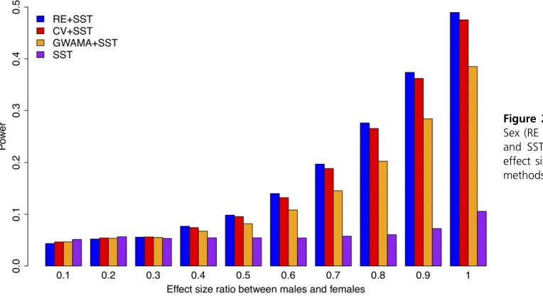
Simulating the sex difference in effect sizes: In the first power simulation, we simulated the effect size difference between the sexes, a phenomenon called“effect size hetero-geneity.”We assumed a SNP of minor allele frequency 0.3 and generated genotypes of 1000 males and 1000 fe-males. Then we simulated continuous phenotypes of these Figure 4 Power characteristics of RE, CV, GWAMA, and SST in a space
individuals while assuming the same error variance for the two sexes. For each male individual, we generated a pheno-type assuming a genetic effect size of 0.192 and variance of 1.0. For each female individual, we generated a phenotype assuming 10% of the male effect size (0.019) and variance of 1.0. We repeated this simulation 10,000 times and computed the power of a method as the proportion of simulations in which the testP-value was more significant than the given significance threshold. We then gradually increased the fe-male effect size from 10 to 100% of the fe-male effect size, to simulate differing levels of heterogeneity.
Figure 2 shows the power of the four approaches (RE + SST, CV + SST, GWAMA + SST, and SST) with respect to the effect size ratio between the two sexes. As expected, when the effect size ratio was very small (when the effect was almost sex-specific), SST showed the highest statistical power. As the effect size of the female study increased, the MetaSex (RE + SST) approach showed the highest statistical power, demonstrating that our approach can effectively de-tect sex-interacting effects. Even at the ratio of 1.0 (when the effect size was identical for both sexes), although CV was expected to be the most powerful, MetaSex (RE + SST) slightly outperformed CV + SST. This was because of our smart thresholding strategy that allowed a more liberal
significance threshold for RE with the expense of a more stringent threshold for SST.
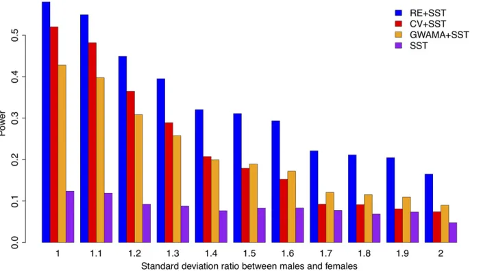
simultaneously varied the effect size ratios and the variance ratios between females and males. In this simulation, RE + SST was still the most powerful (Supplemental Material, Figure S1).
Power characteristics of the methods: We examined why using RE to complement SST was more powerful than using GWAMA or CV to complement SST. We evaluated the power of the individual methods (RE, CV, GWAMA, and SST) over a wide range of female/male genetic effect size pairs, varying each from small value (0) to large value (1.0). Note that although we examined a specific effect size range (0, 1.0), the general tendencies in relative power are expected to be similar in different settings; for example, if the effect sizes were larger and the variances were larger, the power results would be similar. Here, we assumed an error variance ratio of 1.2 (females/males) between the two sexes, because this was
the average ratio of the phenotypic variances in the 10 phe-notypes of the NFBC data.
Figure 4 shows the power of the four individual methods (RE, CV, SST, and GWAMA) in a two-dimensional space wherex-axis is the male genetic effect size andy-axis is the female genetic effect size of a SNP. We plotted the 50% power lines of the four methods, so that each line denotes pairs of the male and female effect sizes where the method achieved an exact power of 50%. Because the power in-creased as the effect size inin-creased, the closer the 50%line was to the bottom leftmost point on the graph, the more powerful the method was. As expected, when one of the effect sizes was close to zero (sex-specific effect: top left cor-ner or bottom right corcor-ner), SST was the most powerful. When the effect sizes were at most moderately different be-tween male and female studies (middle area), RE outper-formed other approaches. We measured the size of the area Figure 6 Association results of RE, CV, GWAMA, and SST in NFBC data. We show 16 SNPs that were associated to one of the 10 phenotypes. (A) Relative
2log10Pimprovement of the other methods compared with the CV method [(2log10Pof RE/GWAMA/SST)2(2log10Pof CV)]. The reference SNP identity
whose power was.50%;which was the area outside of each curve, toward the top right corner. The sizes of the areas were 22:1%for SST, 23:5%for CV, 29:7%for GWAMA, and 29:9% for RE. Thus, RE and GWAMA achieved the largest similar areas.
Figure 4 demonstrates why using RE to complement SST allowed us better power than using GWAMA or CV to com-plement SST in previous simulations (Figure 2 and Figure 3). The GWAMA power line was more steeply curved than the RE power line, which meant that GWAMA tended to detect ef-fects that were extremely different between the sexes. There-fore, what GWAMA found could have substantial overlap to what SST found. The power of the combined methods (RE + SST, CV + SST, and GWAMA + SST) can be interpreted as the sum of areas where each method achieved the power of 50%or more. Figure 4 shows that RE and SST complemented each other resulting in the largest combined area in this plot. To quantify this difference, we measured the area.50%not covered by the 50%power of the SST approach. The areas were 13:8% for GWAMA and 15:4%for RE. Thus, in the common situations that investigators apply SST first, RE can give us the biggest additional power.
We then tested if the three-method compositions, such as RE + CV + SST, RE + GWAMA + SST, and CV + GWAMA + SST, can have better power. We assumed the female effect size of 0.125 and male effect size of 0.25 (effect size ratio of 0.5). We applied the Bonferroni correction to the three-method compositions. Figure S2 shows the power comparison of the seven methods (RE + SST, CV + SST, GWAMA + SST, SST, RE +CV+SST, RE+GWAMA +SST, andCV+GWAMA +SST), where MetaSex (RE + SST) slightly outperformed the others.
Analysis of the NFBC data
We analyzed the NFBC data (Sabattiet al.2009), which con-sisted of 5326 individuals (2546 males and 2780 females). This dataset provided 10 phenotypic measurements of the individuals (seeMaterials and Methods).
Sex difference in phenotypic variances:Wefirst investigated whether the phenotypic variances showed differences be-tween the sexes. We applied Levene’s test, which tests for the equality of the variances between two groups (seeMaterials
and Methods). Table 1 shows thatfive phenotypes (triglycerides, HDL, LDL, BMI, and diastolic blood pressure) showed signif-icant differences in the phenotypic variance between females and males (P,0:005;Bonferroni correction on 10 tests). The most significant difference was observed in triglycerides (P¼1:45310221).
Variance component analysis: To investigate why the phe-notypic variances of some traits differed between the sexes, we performed a variance component analysis. We used thefi ve-variance-component linear mixed model described in Figure 1A, where we excluded the SNP terms. Decomposing the variance components could reveal if the phenotypic variance difference came from the differences in polygenic back-ground effects, or the differences in error variances. We used the Genome-wide Complex Trait Analysis (GCTA) method to perform this analysis (Yanget al.2010). First, we generated the genetic relationship matrix, K; using the GCTA frame-work. Second, we created two modified genetic relationship matrices,K∘hhTandK∘ð12hÞð12hÞT;by masking the val-ues ofKexcept for the sex-specific values (seeMaterials and Methods). Unfortunately, GCTA did not allow us to separate the error term into two sex-specific terms as in the model in Figure 1A, because the default error term (with variances2
e)
for the whole sample was automatically included in the model. Thus, we added the sex-specific error term (with var-iances2
e;ss) to one sex. We tried both males and females for
this additional term, and chose the configuration with
s2 e;ss.0:
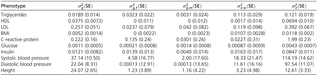
Table 2 and Table S1 show the variance component esti-mates. The polygenic background effect (s2
g) was signifi
-cantly nonzero in five traits (P,0:005 for BMI, HDL, height, LDL, and systolic blood pressure). The sex-interacting polygenic background effects (s2
g;mands2f;m) were nonzero in
some traits, but the SEs were large and none of them showed significance (P.0:005). The variance of the sex-specific er-ror term (s2
e;ss) was significantly nonzero in traits
triglycer-ides (P¼6:2331025) and BMI (P¼1:2031024). Thus, in
some phenotypes, the phenotypic variance difference between the sexes was not completely explained by the genetic compo-nents alone, which suggested the need for explicitly modeling the sex difference in error variances as in our MetaSex method. Table 1 Phenotypic variances in the females and males for the 10 phenotypes of NFBC data
Phenotype Variance (female) Variance (male) Ratio (larger/smaller) Levene’s testP-value
Triglycerides 0.171 0.256 1.494 1.45e221
HDL 0.134 0.107 1.251 2.54e210
LDL 0.670 0.820 1.223 1.39e205
BMI 0.0309 0.0189 1.635 6.14e219
C-reactive protein 2.37 2.24 1.056 0.0877
Glucose 0.0065 0.0068 1.048 0.174
Insulin 0.111 0.117 1.061 0.117
Systolic blood pressure 156.77 171.35 1.092 0.0079
Diastolic blood pressure 118.56 136.05 1.147 0.0012
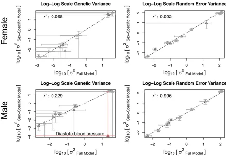
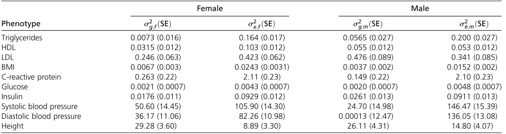
Full model vs. approximated model:Although it was feasible to estimate thefive variance components one time using tools such as GCTA, applying the full linear mixed model to millions of markers can be prohibitively slow because the variance component estimation needs to be repeated for each SNP. Therefore, we proposed an approximated model that decom-poses the problem into two sex-specific linear mixed models (Figure 1B). Here, using the NFBC dataset, we examined if the variance components estimated by the approximated model were similar to those estimated by the full model.
To achieve this goal, we performed GCTA analyses in each sex-specific two-variance-component model described in Fig-ure 1B. Table 3 shows the estimated variance components for the two sexes. We can categorize the variance components into two groups: the genetic variance and the random error variance. The genetic variances in the full and sex-specific models ares2
gþs2g;fðmÞfrom Table 2 ands 2
g;fðmÞfrom Table
3, respectively. The random error variances in the full and sex-specific models are s2
eþs2e;ss from Table 2 (or s2e;
depending on which sex s2
e;ss was added) ands2e;fðmÞ from
Table 3, respectively. We examined if the genetic and random error variances were the same between the full and sex-specific models. Figure 5 shows that the estimated variance components were highly concordant between the full and sex-specific models. Most of the points closely followed the y¼xline (dashed line). The Pearson correlations were high (r2.0:9) in all comparisons, except for the male genetic
variance. The low correlation in the male genetic variance was driven by one outlier (diastolic blood pressure). This outlier appears to have a large SE of the estimates. Specifi -cally, the SE of the genetic variance SEðs2
g;mÞin the sex-specific
model was 12.47, which wasfive orders of magnitude greater than the estimate itself (Table 2). If we excluded this outlier, the correlation was high (r2¼0:979). Overall, the estimates
of the full and sex-specific models were highly concordant, which supported the use of the approximated model in our framework.
Association mapping: We mapped associations for the 10 phenotypes in the NFBC dataset, using different methods. We used our efficient approximated model; that is, in each sex, we
applied a sex-specific linear mixed model (Efficient Mixed-Model Association eXpedited (EMMAX); Kang et al. 2010) to account for the polygenic effects and the sex-interacting polygenic effect simultaneously (Figure 1B). Then, we applied RE and SST to the resulting female and male effect size esti-mates. For comparison, we also applied CV and GWAMA. In both CV and GWAMA, we similarly accounted for the poly-genic background effects using variance components. Finally, for a fair comparison, we calculated the genomic control fac-torlseparately for each method (Table S2) and corrected the resultingP-values of each method, using this factor.
The challenge in this real dataset analysis was the lack of an objective measure to compare performances of the methods because we do not know which loci are true positives. What we could do was to examine loci that were genome-wide signif-icant and compare theP-values of different methods. Under the assumption that the loci exceeding the significance threshold have a high chance of being true positives, a puta-tively better method can be a method that gave smallerP-values at those loci.
In this analysis, we discovered 16 loci that were associated with any of the 10 phenotypes at the threshold level P,531028 by at least one method. At these 16 loci, we
calculated theP-values using RE, CV, GWAMA, and SST (Ta-ble S3). To compare theP-values of the methods, we chose CV as a reference method. We plotted the2log10Pdifference
between each method and the CV approach in Figure 6A [(2log10Pof RE/GWAMA/SST)2(2log10Pof CV)]. Thus,
for each SNP, the positively larger the difference, the better the method was compared with CV. As shown in Figure 6A, RE showed the best overall performance. RE gave smaller P-values than GWAMA at 14 out of 16 loci and betterP-values than CV at 11 out of 16 loci. Even at loci where GWAMA or CV showed smallerP-values than RE, the difference from RE was small. Specifically, REP-values were never larger by one or-der of magnitude than any of these methods at all 16 loci.
We further investigated on what characteristics of the loci caused theseP-value differences between the methods. First, Figure 6B shows the phenotype variance ratio (PVR) between males and females after regressing out the genetic effect of the SNP tested. Second, Figure 6C shows the effect size ratio Table 2 Variance components in the fullfive-variance-component model for the 10 phenotypes of NFBC data
Phenotype s2
gðSEÞ s2g;fðSEÞ s2g;mðSEÞ s2e;ssðSEÞ s2eðSEÞ Triglycerides 0.0189 (0.014) 0.0323 (0.022) 0.0031 (0.024) 0.113 (0.029) 0.121 (0.019) HDL 0.0375 (0.0072) 0 (0.011) 0 (0.012) 0.0017 (0.014) 0.0694 (0.010) LDL 0.257 (0.051) 0.0237 (0.079) 0.042 (0.082) 0.119 (0.098) 0.392 (0.067) BMI 0.0052 (0.0014) 0 (0.0022) 0 (0.0023) 0.0107 (0.0028) 0.0118 (0.002) C-reactive protein 0.222 (0.16) 0.135 (0.24) 0.0301 (0.26) 0.0227 (0.31) 1.99 (0.23) Glucose 0.0011 (0.0005) 0.00021 (0.0008) 0.0014 (0.0008) 0.00087 (0.0009) 0.0043 (0.0007) Insulin 0.0121 (0.0082) 0.0139 (0.013) 0.0040 (0.014) 0.0163 (0.017) 0.0847 (0.011) Systolic blood pressure 37.14 (10.50) 4.58 (16.77) 2.00 (17.60) 18.33 (21.47) 114.19 (14.62) Diastolic blood pressure 22.04 (8.31) 0.00013 (12.91) 0.00013 (13.65) 11.61 (16.16) 97.54 (11.07) Height 24.07 (2.65) 1.23 (3.89) 1.16 (4.22) 3.23 (4.98) 12.61 (3.33)
s2
g;polygenic background effects;s2g;f;female-specific polygenic background effects;s2g;m;male-specific polygenic background effects;s2e;ss;sex-specific random errors;s2e;
between males and females for each SNP. Because the power of the methods depend on both the error variance ratio (which will affect PVR) and the effect size ratio be-tween males and females as we have shown in simula-tions, we can interpret theP-values of the methods (Figure 6A) in terms of the PVR (Figure 6B) and the effect size ratio (Figure 6C).
If we look at the SNP rs7298683 (indicated byy, Figure 6), the effect size ratio between males and females was20.0227 (Table S3), which meant that the effect direction was oppo-site for the two sexes and that the absolute magnitude of the male effect size was 36 times larger than that of the female effect size. However, there was almost no difference in PVR between male and female studies (PVR of 0.965). In this case, the SST approach gave the smallestP-value, because SST was the best method to detect an extreme effect size magnitude difference as we have shown in simulations.
If we look at the SNP rs2167079 (indicated by *, Figure 6), the PVR (female/male) was 1.261 and the effect size ratio (female/male) was 0.43 (Table S3). The variance in females was larger, so the female effect size estimate was more un-certain than the male estimate. Thus, when combining infor-mation from the two sexes, an optimal method should give more weight to male estimate. Moreover, effect size was greater in males. Thus, an optimal method should give more weight to the male estimate even further. Because CV ignores both the variance difference and the effect size difference, RE achieved a smaller P-value at this locus than CV. A similar interpretation of the result can be applied to the SNPs rs7120118 and rs693 (indicated by
•
, Figure 6).Now consider the SNP rs11668477 (indicated by‡, Figure 6). The PVR (female/male) was 0.82 and the effect size ratio (female/male) was 0.5 (Table S3). In this case, when com-bining information from the two sexes, based on the variance, we should weight the female estimate, but based on the effect size, we should weight the male estimate. Thus, the effect of differing variances and the effect of differing effect sizes can-celed out, giving CV the smallest P-value of all approaches because CV can be considered as equally weighting the two sexes. A similar interpretation of the result can be applied to the SNPs rs2794520, rs560887, and rs10096633 (indicated
by ), Figure 6). However, as described, even in such situa-tions, RE was not much worse than CV.
In summary, RE showed the best stable performance of all methods, except when the effect only existed in one sex where SST performed the best. This analysis demonstrates that our MetaSex framework, where RE and SST complement each other, can cover many possible situations with high power.
Discussion
Here, we present MetaSex, a novel framework that accounts for the potential sex difference in genetic architectures for powerful association mapping. We built our method on a comprehensive model that included multiple variance com-ponents and expedited the optimization by using an approx-imated sex-specific models. We utilized the meta-analysis framework to achieve high power in a wide range of situations. Simulations and real data analyses supported the superior per-formance of our approach compared with previous approaches. The high power of our approach was attributable to two factors: the effect size difference between the sexes and the error variance difference between the sexes. Previous studies have observed effect size differences at a number of loci (Randall et al. 2013; Winkler et al. 2015). However, few studies have reported phenotypic variance differences be-tween the sexes, which can reflect the error variance differ-ence. In our study, we showed that the phenotypic variance difference can be a real phenomenon in the existing dataset. The nongenetic cause of the phenotypic variance difference can be sex acting as an environment (e.g., hormone) or sex interacting with external environments (e.g., lifestyle). We demonstrated that accounting for the nongenetic causes by modeling differing error variances can increase power.
Our framework can be generalized to analyze data con-taining any strata other than the sex. To apply our framework to N strata, we can apply the linear mixed model to each stratum and obtainNeffect size estimates and their SE. First, we can perform stratum-specific tests with the estimated ef-fect sizes. Next, we use those estimates as an input to RE and perform a meta-analysis for multiple strata. Finally, we can correct for multiple testing of the RE andNstratum-specific Table 3 Variance components in the sex-specific models for the 10 phenotypes of NFBC data
Female Male
Phenotype s2
g;fðSEÞ s2e;fðSEÞ s2g;mðSEÞ s2e;mðSEÞ
Triglycerides 0.0073 (0.016) 0.164 (0.017) 0.0565 (0.027) 0.200 (0.027) HDL 0.0315 (0.012) 0.103 (0.012) 0.055 (0.012) 0.053 (0.012) LDL 0.246 (0.063) 0.423 (0.062) 0.476 (0.089) 0.341 (0.085) BMI 0.0067 (0.003) 0.0243 (0.0031) 0.0037 (0.002) 0.0152 (0.002) C-reactive protein 0.263 (0.22) 2.11 (0.23) 0.149 (0.22) 2.10 (0.23) Glucose 0.0021 (0.0007) 0.0043 (0.0007) 0.0020 (0.0007) 0.0048 (0.0007) Insulin 0.0176 (0.011) 0.0929 (0.012) 0.0261 (0.013) 0.0911 (0.013) Systolic blood pressure 50.60 (14.45) 105.90 (14.30) 24.70 (14.98) 146.47 (15.39) Diastolic blood pressure 36.17 (11.06) 82.26 (10.98) 0.00013 (12.47) 136.05 (13.08) Height 29.28 (3.60) 8.89 (3.30) 26.11 (4.31) 14.80 (4.07)
s2
tests by the smart thresholding strategy, where the thresholds can be calculated for a specific situation.
In our simulations, we assumed that the effects of the two sexes are in the same direction. Our assumption was that for disease phenotypes, it would be rare that the same variant increases risk for one sex and decreases for the other. The results of the NFBC dataset supported this assumption, given that none of the 16 associated variants showed significant evidence of opposite effects (Table S3). In a recent study, some variants were found to be associated to waist/hip ratio in males and females in an opposite way (Winkleret al.2015). We tried an extended simulation setup to test variants with opposite effects (Figure S3). Among the four approaches (RE + SST, CV + SST, GWAMA + SST, and SST), GWAMA + SST achieved the highest power if the directions were opposite. This indicates that RE and GWAMA can play a different role in the analysis; RE is powerful for detecting unidirectional effects while GWAMA is powerful for detecting opposite effects.
We did not systematically compare the runtime of the methods (MetaSex, CV + SST, and GWAMA + SST) because the runtime greatly depends on the specific implementation of the linear mixed model that is applied to each sex. Because the meta-analytic part (RE or GWAMA) only combines two esti-mates (female and male effect sizes), the runtime for meta-analysis is relatively negligible. Zhou and Stephens compared the runtimes of the standard linear mixed models for two variance components (Zhou and Stephens 2012), which showed that the recent implementations of the linear mixed model can be applied to the typical GWAS dataset within a single day. Therefore, if we use these implementations for each sex, the time complexity of the whole procedure of our framework will be similar.
Although we tried to account for many possible phenom-ena that can occur due to the sex difference in genetic association mapping, our model might still have limitations. In our method, we explicitly modeled the sex difference in the effect sizes of the associated locus, magnitudes of the poly-genic effects, and error variances. However, we did not model the sex difference in the phenotype distribution (i.e., shape), genetic interaction with CVs, or the liability distribution of binary traits. Moreover, we only assumed a specific parame-ter space or dataset both in power evaluations and in variance estimate comparison of the full and approximated models. In future analyses, extended datasets or simulations may help us evaluate the full characteristics of our method in the wider spectrum of situations. We expect that a large-scale study will be necessary to fully decipher sex-interacting genetic archi-tectures of human traits.
Acknowledgments
C.H.L. and B.H. are supported by the National Research Foundation of Korea (NRF) grant (grant number 2016R1C1B2013126) and the Bio & Medical Technology Development Program of the NRF (grant number 2017M3A9B6061852) funded by the Korean government,
Ministry of Science and ICT. E.Y.K., N.A.F., J.W.J.J., E.K., N.Z., and E.E. are supported by National Science Foundation grants 0513612, 0731455, 0729049, 0916676, 1065276, 1302448, 1320589, and 1331176, and National Institutes of Health grants K25-HL080079, U01-DA024417, P01-HL30568, P01-HL28481, R01-GM083198, R01-ES021801, R01-MH101782, and R01-ES022282. The authors declare no conflict of interest.
Literature Cited
Aschard, H., D. B. Hancock, S. J. London, and P. Kraft, 2010 Genome-wide meta-analysis of joint tests for genetic and gene-environment interaction effects. Hum. Hered. 70: 292–300.https://doi.org/10.1159/000323318
Boraska, V., A. Jeronči´c, V. Colonna, L. Southam, D. R. Nyholtet al., 2012 Genome-wide meta-analysis of common variant differ-ences between men and women. Hum. Mol. Genet. 21: 4805– 4815.https://doi.org/10.1093/hmg/dds304
Brown, M. B., and A. B. Forsythe, 1974 Robust tests for the equal-ity of variances. J. Am. Stat. Assoc. 69: 364–367.
Chen, Y. C., G. H. Dong, K. C. Lin, and Y. L. Lee, 2013 Gender difference of childhood overweight and obesity in predicting the risk of incident asthma: a systematic review and meta-analysis. Obes. Rev. 14: 222–231. https://doi.org/10.1111/j.1467-789X.2012.01055.x
DerSimonian, R., and N. Laird, 1986 Meta-analysis in clinical tri-als. Control. Clin. Trials 7: 177–188.https://doi.org/10.1016/ 0197-2456(86)90046-2
Eskin, E., 2008 Increasing power in association studies by using linkage disequilibrium structure and molecular function as prior information. Genome Res. 18: 653–660. https://doi.org/ 10.1101/gr.072785.107
Fox, C. S., Y. Liu, C. C. White, M. Feitosa, A. V. Smith et al., 2012 Genome-wide association for abdominal subcutaneous and visceral adipose reveals a novel locus for visceral fat in women. PLoS Genet. 8: e1002695. https://doi.org/10.1371/ journal.pgen.1002695
Han, B., and E. Eskin, 2011 Random-effects model aimed at dis-covering associations in meta-analysis of genome-wide associa-tion studies. Am. J. Hum. Genet. 88: 586–598.https://doi.org/ 10.1016/j.ajhg.2011.04.014
Hardy, R. J., and S. G. Thompson, 1996 A likelihood approach to meta-analysis with random effects. Stat. Med. 15: 619–629. https://doi.org/10.1002/(SICI)1097-0258(19960330)15:6,619:: AID-SIM188.3.0.CO;2-A
Kang, E. Y., B. Han, N. Furlotte, J. W. J. Joo, D. Shih et al., 2014 Meta-analysis identifies gene-by-environment interac-tions as demonstrated in a study of 4,965 mice. PLoS Genet. 10: e1004022.https://doi.org/10.1371/journal.pgen.1004022 Kang, H. M., N. A. Zaitlen, C. M. Wade, A. Kirby, D. Heckerman et al., 2008 Efficient control of population structure in model organism association mapping. Genetics 178: 1709–1723. https://doi.org/10.1534/genetics.107.080101
Kang, H. M., J. H. Sul, S. K. Service, N. A. Zaitlen, S.-Y. Y. Kong et al., 2010 Variance component model to account for sample structure in genome-wide association studies. Nat. Genet. 42: 348–354.https://doi.org/10.1038/ng.548
Kostis, W. J., J. Q. Cheng, J. M. Dobrzynski, J. Cabrera, and J. B. Kostis, 2012 Meta-analysis of statin effects in womenvs.men. J. Am. Coll. Cardiol. 59: 572–582. https://doi.org/10.1016/j. jacc.2011.09.067
waist circumference and the risk of barrett’s oesophagus: a pooled analysis from the international beacon consortium. Gut 62: 1684– 1691.https://doi.org/10.1136/gutjnl-2012-303753
Lippert, C., J. Listgarten, Y. Liu, C. M. Kadie, R. I. Davidsonet al., 2011 Fast linear mixed models for genome-wide association studies. Nat. Methods 8: 833–835. https://doi.org/10.1038/ nmeth.1681
Magi, R., C. M. Lindgren, and A. P. Morris, 2010 Meta-analysis of sex-specific genome-wide association studies. Genet. Epidemiol. 34: 846–853.https://doi.org/10.1002/gepi.20540
Mason, B. J., and P. Lehert, 2012 Acamprosate for alcohol de-pendence: a sex-specific meta-analysis based on individual patient data. Alcohol. Clin. Exp. Res. 36: 497–508. https:// doi.org/10.1111/j.1530-0277.2011.01616.x
Ohmen, J., E. Y. Kang, X. Li, J. W. Joo, F. Hormozdiari et al., 2014 Genome-wide association study for age-related hearing loss (ahl) in the mouse: a meta-analysis. J. Assoc. Res. Otolar-yngol. 15: 335–352. https://doi.org/10.1007/s10162-014-0443-2
Peters, S. A. E., R. R. Huxley, and M. Woodward, 2013 Comparison of the sex-specific associations between systolic blood pressure and the risk of cardiovascular disease: a systematic review and meta-analysis of 124 cohort studies, including 1.2 million in-dividuals. Stroke 44: 2394–2401. https://doi.org/10.1161/ STROKEAHA.113.001624
Porcu, E., M. Medici, G. Pistis, C. B. Volpato, S. G. Wilson et al., 2013 A meta-analysis of thyroid-related traits reveals novel
loci and gender-specific differences in the regulation of thyroid function. PLoS Genet. 9: e1003266. https://doi.org/10.1371/ journal.pgen.1003266
Randall, J. C., T. W. Winkler, Z. Kutalik, S. I. Berndt, A. U. Jackson et al., 2013 Sex-stratified genome-wide association studies in-cluding 270,000 individuals show sexual dimorphism in genetic loci for anthropometric traits. PLoS Genet. 9: e1003500. https://doi.org/10.1371/journal.pgen.1003500
Sabatti, C., S. K. Service, A.-L. L. Hartikainen, A. Pouta, S. Ripatti et al., 2009 Genome-wide association analysis of metabolic traits in a birth cohort from a founder population. Nat. Genet. 41: 35–46.https://doi.org/10.1038/ng.271
Winkler, T. W., A. E. Justice, M. Graff, L. Barata, M. F. Feitosaet al., 2015 The influence of age and sex on genetic associations with adult body size and shape: a large-scale genome-wide interac-tion study. PLoS Genet. 11: e1005378 [corrigenda: PLoS Genet. 12: e1006166 (2016)]. https://doi.org/10.1371/journal.pgen. 1005378
Yang, J., B. Benyamin, B. P. McEvoy, S. Gordon, A. K. Henderset al., 2010 Common snps explain a large proportion of the herita-bility for human height. Nat. Genet. 42: 565–569.https://doi. org/10.1038/ng.608
Zhou, X., and M. Stephens, 2012 Genome-wide efficient mixed-model analysis for association studies. Nat. Genet. 44: 821–824. https://doi.org/10.1038/ng.2310