Amplifier
Quang Quy Ho1, Van Bien Chu2
1NewTechPro, Vietnam Academy of Science and Technology, Hanoi, Vietnam; 2Physical Faculty, Hongduc University, Thanh Hóa,
Vietnam.
Email: [email protected]; [email protected]
Received July 7th, 2012; revised August 9th, 2012; accepted August 18th, 2012
ABSTRACT
Based on the nonlinearity of the nonlinear optical coupler (NOC) and the amplifying capacity of the backward Raman fiber amplifier (PBRFA), two new optical systems to compress the optical pulse (Optical Pulse Self-Compressor: OPSC) are proposed. Using the expressions describing relationship between input and output intensities from ports of the NOC and the derived expression describing the amplification of the PBRFA, the compressing process of the optical pulse propagating through the OPSC is simulated. The results show that the peak of the optical pulse will be enhanced and the duration of the optical pulse will be reduced significantly. Consequently, the shape of input pulse is completely com- pressed with the certain efficiency. It means the optical pulse is self-compressed without the external pump pulse by proposing the OPSC.
Keywords: Backward Raman Fiber Amplification; Nonlinear Optical Coupler (Integrated-Optical Direction Coupler); Pulse Compression
1. Introduction
There are many techniques interested and used to com- press the optical pulse as the amplitude passive modula- tion, the mode-locking, the intra-cavity saturation absor- ption-amplification [1,2], the stimulated Raman back- scattering in plasma [3-22], etc. The operating principle of all mentioned techniques is based on the nonlinearity in the optical medium under the interaction of the intense laser beam [2,3,8,12,23]. In the early 1970s, Stolen and Ippen [24] demonstrated Raman amplification in optical fibers. By the early part of 2000s, almost every long-haul (typically defined ~300 km to 800 km) or ultralong-haul (above 800 km) fiber-optic transmission system uses Ra- man amplification [6], and there are many works inter- ested in the stimulated Raman backscattering in fiber [25, 26]. As the operating principle of the pumped backward Raman amplification, the longer pulse propagating along the opposite direction of the signal pulse is needed. So, the classical pulse compressing system always needs two optical pulses, of which one plays the role of the pump source and the one plays the role of the signal.
In our previous works [27,28], the nonlinear optical coupler has been proposed and the nonlinearity appeared in the transfer efficiency-input intensity characteristic.
Due to the nonlinearity of the nonlinear optical coupler, the output pulse selection at two ports is found out, i.e.
when the powerful signal is propagated through one port, meanwhile the weak signal will propagate through the second port in the conditional intensity density. The in- tensity reducing at the second port of the NOC can be seen as the phenomenon appeared in the saturation ab- sorption medium. Thus, the combination of the nonlinear optical coupler (NOC) with the pumped backward Ra- man fiber amplifier (PBRFA) will become a system to compress the optical pulse.
In this paper, we propose the configuration of two op- tical pulse self-compressors (OPSC) based on the NOC and the PBRFA. The simulated results will be presented to confirm the pulse self-compression possibility of the proposed OPSC.
2. Arguments
2.1. Intensity Selection and Pulse Shortening of NOC
Figure 1. Nonlinear optical coupler.
coupler except for the Kerr effect in nonlinear fiber [26]. Because of the Kerr effect, the transfer coefficients lin at output linear port and at output nonlinear port of the NOC depend on input intensity, which are given as follows [27,28]:
1
nonlin
2 2 4 4
2
2 0 2
2 2 4 4
2 0
2 2 4 4
2
2 0 2
2 2 4 4
2 0 sin 16 16 1 1 sin 16 16 nl in lin cpl nl in nonlin nl in cpl nl in n I C l C n I C n I C l C n I C (1)
where, ω is the signal frequency, ε0 is the electric per-
meability, Iin is the input intensity, out lin, is the out-
put intensity from output port of linear fiber, out nonlin, is
the output intensity from output port of nonlinear fiber (see Figure 1), nl is the nonlinear coefficient of re- fractive index of nonlinear fiber, cpl is the coupling length, and C is the linear coupling coefficient, which depends on the radius of fiber, separation distance be- tween two fibers, refractive index, and signal wavelength [29].
I I
n
l
Consider the parameters of the NOC are as follows: ,
0.694/mm
C 1.0 10 12mm2
nl
n W , lcpl = 2.5 mm. The transmittance efficiency-input intensity characteris- tics at two ports are simulated for the optical beam with its wavelength 1.5μm, and illustrated in Figure 2. From Figure 2, we can see that, with given parameters of the NOC (i.e. with designed NOC), a laser signal at wavelength of1.5 m will be transmitted from the linear output port if its intensity density is more than about 20 1012 W/mm2, meanwhile transferred to nonlinear output
port if its intensity density is less than 5 1012 W/mm
[27]. It means that the NOC has the property of intensity selection, which is presented in Figure 3. From Figure 3, we can see that, the considered input pulse is Gaussian,
i.e.
Figure 2.The transfer efficiency through liner output port (solid) and nonlinear output port (dot) of NOC with nnl =
1.0 × 10⁻¹² mm2/W, l
cpl = 2.5 mm vs input intensity density at λ = 1.5 μm.
Figure 3. Output pulses from two ports of NOC.
max, exp ln 2 22in in
t
I t I
(2)
with peak intensity density 12 2 max,in 4 10 W mm
I
and half-duration , is split into two parts, the intense pulse, out lin, , with slight changing of the peak intensity density and duration, has gone out from the linear output port, meanwhile the weak one, out nonlin, ,
with big reduction of both peak and duration, from the nonlinear output port.
9
1 10 s
I
I
It is important that the duration of weak pulse from nonlinear output port is reduced to . This pro- perty of the NOC gives us an idea to set up the pulse compression system consisted of the NOC and the PBRFA (i.e. OPSC). For this OPSC, the intense pulse can be used as pumping pulse for PBRFA, and the weak shorten pulse will be amplified as the signal pulse.
9
0.5 10 s
(a)
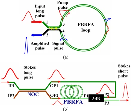
[image:3.595.62.285.95.281.2](b)
Figure 4. Set-up of OPSC. (a) OSPC consist of the NOC and PBRFA loop; (b) OSPC consist of the NOC and PBRFA and 3 dB.
from output port (3), which is injected into the PBRFA as the pump pulse, and guided to the second output port (4) along the clock-hand direction (assumed − z direction). Meanwhile, the weak and shorter pulse will go out from the output port (4), which is injected into the PBRFA as the signal pulse, and guided to port (3) along the opposite clock-hand direction (assumed + z direction). This pulse will be amplified by stimulated Raman backscattering [30] and go out from port (2) with a slight changing.
For the second model in Figure 4(b), a long Stokes pulse is injected into the NOC through input port (PI1). After propagating through the NOC, the more intense pulse will go out from the output port (OP1), which is injected into the PBRFA through port P2 and P1 of the 3 dB coupler as the pump pulse along −z direction. Mean- while, the weak and shorter one will go out from the second output port of the NOC (OP2), which is injected into PBRFA as the signal pulse along +z direction. This pulse will be amplified by stimulated Raman backscat-tering and go out from port P3 of the 3 dB coupler.
2.3. Signal Gain of the PBRFA
For example, we derive the expression of amplified pulse for the first model. Consider the PBRFA is a single-mode fiber with length L. The signal pulse from port (4) is in- jected at z = 0 and travels in the +z direction (along op- posite clock-hand direction), while the pump pulse from port (3) with peak power, Pmax,p [W], and duration, 2 τ [s], is injected at z = L and propagates along –z direction (along clock-hand direction). Let [dB/km] be the loss coefficient of the signal and let g [m/W] and A [m2]
denote the Raman gain constant and the effective Raman cross section, respectively.
site direction of the pump pulse, the interaction length is
int g
L v [m], which is chosen to be the length of the PBRFA’s fiber, where vg is the group velocity of pulse. At each point of this interval, (or ) the pump amplitude is considered as i g
z v ti ti
2
intmax , 2 int
int
exp ln 2 exp
p i i p p P z z L P z L
i
L (3)
Similar to that of work of Lin and Stolen [31], the sig- nal gain obtained from the pump pulse is given by
exp
i i igP z z G z
A
(4) However, at every point the signal pulse has the propa- gation loss es iz . Hence the net gain is given as
exp
i ii s
gP z z
G z z
A
i (5) As shown in Figure 3, the pump pulse is more longer than the signal pulse, so in distance increment, z
g s
v , where s is the duration of signal pulse, the gain coefficient is considered to be constant, i.e. G
zi
iG z , and the signal is enhanced by factor G z
i , thatmeans the output signal pulse after propagating through i
z
can be expressed as [32]
. , ,
out s i i in s i
P t z G z P t n z (6)
where, n z
i is the quantum noise at point zi [16,21],
,
in s
P t
z
is the input signal pulse injected into the incre-ment i.
We assume the loss and quantum noise are small neg- ligible, using (5) and (6), we have
int , 1 , 1 , exp Namp in s i
i N
i i in s
i
P t L P t G z
gP z z
P t A
(7)where N p s s.
The signal pulse travels along the opposite direction of the pump pulse, the shape of its can be expressed as fol-lows
2 i ,
, ax,s 2
,
exp ln2 n s i
in s i m
in s
L z
P z P
L (8)
After replacing the length argument i by the time argument t, and substituting (3), (8) into (7), we have
z
2
, ax,s 2
2 ax,p
2 1
exp ln2
exp exp ln2
s amp s m
s N
g i m i
i
t
P t P
gv t P t
A
(9)which describes the shape of the amplified pulse propa-gated through PBRFA only.
To have the shape of the output amplified pulse from port (2) of the NOC, we must combine (1) with (9). Firstly, resolving (1) to find out Pmax ,s, s and Pmax ,p; next, substituting them into (9) to find out Pamp s,
t ; finally, using (1) again to find out the output amplified pulse. In the simulating process, we can replace the in- tensity P with the intensity density: W P A [W/m2],then (9) can be rewritten as follows
2
, ax, 2
2
ax, 2
1
exp ln2
-exp exp ln2
s amp s m s
s N
i g i m p
i
t
W t W
t gv t W
(10)For the second model in Figure 4(b), to obtain the amplified pulse, the expression (1), (9) and (10) will be used also, but the simulation process is slightly changed,
i.e., firstly, resolving (1) to find out Pmax,s, s and
max,p
P ; secondly, multiply Pmax,p with 1/2 (by 3 dB coupler), thirdly, substituting them into (9) to find out ; fourthly, using (1) again to find out the output amplified pulse, finally, multiply again with 1/2. amp s,
P t
2.4. Simulation of the Self-Compression Process All the NOC’s parameters are given in Section 2.1. The input signal pulse parameters are as follows: Wmax,in
12 2
1.0 10 W m
, . The PBRFA parame-
ters are as follows:
6
1 10 s
13
1.0 10 m
g W , 2 10 m s8
g
v
[33], and Lt vg 200 m.
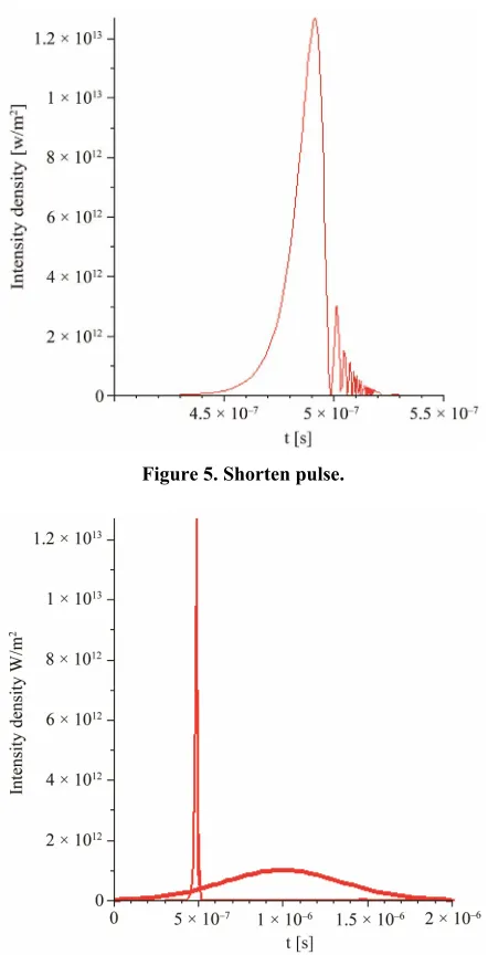
For parameters given above, the shorten pulse is simu- lated (Figure 5), and compared with the input pulse ( Fig-ure 6). From Figure 5, we see that, the duration of opti- cal pulse is shorten about , i.e. about 102 times
shorter, meanwhile, its peak intensity density is enhanced to
8
2 10 s
13 2
1.3 10 W m .
Let
d max πln 2
E W t t W
be the energy den-sity and the ratio of input pulse to amplified pulse, energ E Ein amp
be energy transfer efficiency. Let
max 2
F W be defined as the pulse “force” and
comp Famp Fin
as the compression efficiency. Then, from Figure 5 we can see that although the energy trans- fer efficiency reaches 13% only, which means the energy density of pump pulse is not changed in good agreement with our approximation, but the duration of the amplified pulse is significantly reduced, about 10–2 times shorter.
Additionally, the force, Famp, of the amplified pulse in- creases up to , much bigger than that, in
21
0.65 10 F , of
the input pulse, . It means, the self-compress- ing efficiency for our model,
18
0 0.5 1
comp
, is very high at about (see Table 1).
3
1.3 10
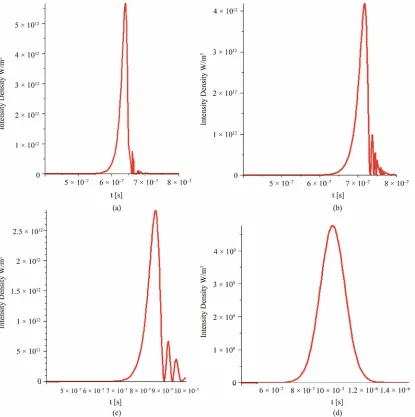
[image:4.595.64.288.127.197.2]However, the shorten pulse’s shape, i.e. its peak power and duration as well as compressing efficiency depend on the designing parameters, for example, their shape depends on the Raman gain in Figure 7.
Figure 5. Shorten pulse.
[image:4.595.313.534.288.720.2]Figure 7. Self-compressed pulses for different Raman gain: (a) 0.5 × 10⁻¹³ m/W; (b) 0.4 × 10⁻¹³ m/W; (c) 0.3 × 10⁻¹³ m/W; (d)
0.2 × 10⁻¹³ m/W.
Table 1. Parameters of the compressed pulses vs the Raman gain.
g [m/W] 0.2 × 10⁻¹³ 0.3 × 10⁻¹³ 0.4 × 10⁻¹³ 0.5 × 10⁻¹³ 1.0 × 10⁻¹³
Wmax [W/m2] 4.6 × 10⁹ 2.8 × 10¹² 4.2 × 10¹² 5.6 × 10¹² 1.3 × 10¹³
τ [s] 1 × 10⁻⁷ 0.5 × 10⁻⁷ 0.35 × 10⁻⁷ 0.12 × 10⁻⁷ 0.1 × 10⁻⁷
F [W/m2·s] 2.3 × 10¹⁶ 2.8 × 10¹⁹ 6 × 10¹⁹ 4.35 × 10²⁰ 0.65 × 10²¹
ηcomp [*] 4.6 × 10⁻² 5.6 × 101 1.2 × 10² 8.7 × 10² 1.3 × 10³ *F
in = 0.5 × 10¹⁸.
If the Raman gain constant increases, the peak power of the amplified pulses increases, meanwhile, their dura-tion decreases.
backward Raman fiber amplifier, the optical pulse self- compressor was newly proposed. The pulse selection at two ports of the NOC is shown out by the simulation. This property is a main reason to choose output pulses from the NOC as the pump and the signal pulses for the PBRFA. With proposed configuration of the self-com-
3. Conclusion
[image:5.595.55.541.568.639.2]pressor, the expression for the amplified pulse was in-troduced by some approximations. The simulated results have shown that by these configurations, the optical pulse should be self-compressed with a certain efficiency, which can be enhanced by the matching conditions. However, the quality of the OPSC, especially, the com- pression efficiency, depends on the principle parameters as the nonlinear coefficient of the refractive index, coup- ling length, radius of fiber core, peak intensity density and duration of input pulse, etc. Those questions will be investigated in detail in next articles.
REFERENCES
[1] L. V. Taracov, “Laser Physics,” Mir, Moscow, 1988, pp. 214-335.
[2] G. H. He and S. H. Liu, “Physics of Nonlinear Optics,” World Scientific Publishing Co. Pte Ltd., Singapore, 1999. [3] E. V. Ermolaeva and V. G. Bespalov, “Optimum Condi-
tions for Stimulated Raman Scattering, Compression, and Amplification of Supershort Pulses in a Plasma with Com- pressed Gases,”Journal of Optical Technology, Vol. 74, No. 11, 2007, pp. 734-739.
[4] J. Wu and M. S. Kao, “Light Amplification Using Back- ward Raman Pumping,” Microwave and Optical Tech- nology Letters, Vol. 1, No. 4, 1988, pp. 129-131.
doi:10.1002/mop.4650010406
[5] J. R. Murray, J. Goldhar, D. Eimerl and A. Szoke, “High-Eficiency Energy Extraction in Backward-Wave Raman Scattering,” IEEE Journal of Quantum Electron-ics, Vol. 15, No. 5, 1979, pp. 342-368.
doi:10.1109/JQE.1979.1070009
[6] M. N. Islam, “Raman Amplifiers for Telecommunica- tions,” IEEE Journal of Selected Topics in Quantum, Vol. 8, No. 3, 2002, pp. 548-559.
[7] J. Kim, H. J. Lee, H. Suk and I. S. Ko, “Solitary Wave Generation by Two Counter-Propagating Laser Pulses in a Plazma”Physics Letters A, Vol. 314, No. 5-6, 2003, pp. 464-471. doi:10.1016/S0375-9601(03)00944-7
[8] V. L. Kalashnikov, “Pulse Shortening in the Passive Q- Switched Lasers with Intracavity Stimulated Raman Scat- tering,” Optics Communications, Vol. 218, No. 1-3, 2003, pp. 147-153. doi:10.1016/S0030-4018(03)01191-X [9] V. M. Malkin N. J. Fisch and J. S. Wurtele, “Compres-
sion of Powerful x-Ray Pulses to Atto-Second Durations by Stimulated Raman Backscattering in Plasmas,” Physi- cal Review Letters, Vol. 75, No. 2, 2007, Article ID: 026404. doi:10.1103/PhysRevE.75.026404
[10] E. Dewald, et al., “Amplification of 1 Pico-Second Pulse Length Beam by Stimulated Raman Scattering of 1 ns Beam in Low Density Plasma,” UCRL-CONF-213152, 2005.
[11] J. Wu, F. Luo and M. Cao, “Generation of Ultrafast Pulse via Combined Effect of Stimulated Raman Scattering and Non-Degenerate Two-Photon Absorption in Silicon Nano- photonic Chip,” Pramana—Journal of Physics, Vol. 72,
No. 40, 2009, pp. 727-734.
[12] I. P. Prokopovich and A. A. Khrushchinskii, “Highly Efficient Generation of Attosecond Pulses in Coherent Stimulated Raman Self-Scattering of Intense Demtosec-ond Laser Pulses,” Laser Physics, Vol. 7, No. 2, 1997, pp. 305-308.
[13] E. M. Dianov, “Raman Fiber Amplifier for the Spectral Region near 1.3 μm,” Laser Physics, Vol. 6, No. 3, 1996, pp. 579-581.
[14] P. A. Apanasevich, et al., “Compression of Laser Pulse in the Interaction of Counterpropagating Waves in a Me- dium with an Inertial Cubic Nonlinearity,” Laser Physics, Vol. 6, No. 6, 1996, pp. 1050-1055.
[15] M. Conforti, et al., “Pulse Shaping via Backward Second Harmonic Generation,” Optics Express, Vol. 16, No. 3, 2008, p. 2115. doi:10.1364/OE.16.002115
[16] Y. Ping, et al., “Amplification of Ultra-Short Laser Pulses by a Resonant Raman Scheme in a Gas-Jet Plasma,” Physical Review Letters, Vol. 92, No. 17, 2004, Article ID: 175001. doi:10.1103/PhysRevLett.92.175007 [17] A. A. Balakin, et al., “Backward Raman Amplification in
Partially Ionized Gas,” Physical Review E, Vol. 72, No. 3, 2005, Article ID: 036401.
doi:10.1103/PhysRevE.72.036401
[18] C. H. Pai, et al., “Backward Raman Amplification in Plasma Waveguide,” Physical Review Letters, Vol. 101, No. 6, 2008, Article ID: 065005.
[19] V. M. Malkin and N. J. Fisch, “Backward Raman Ampli- fication of Ionizing Laser Pulses,” Physics of Plasmas, Vol. 8, No. 10, 2001, p. 4698. doi:10.1063/1.1400791 [20] V. M. Malkin and N. J. Fisch, “Short-Pulse Laser Ampli-
fication and Saturation Using Stimulated Raman Back- scattering and Amplification in a Gas Jet Plasma,” Phys-ics of Plasmas, Vol. 17, No. 7, 2010, Article ID: 073109. doi:10.1063/1.3460347
[21] E. V. Ermolaeva and V. G. Bespalov, “Optimum Condi- tions for Stimulated Raman Scattering, Compression and Amplification of Supershort Pulses in a Plasma with Com- pressed Gases,” Journal of Optical Technology, Vol. 74, No. 11, 2007, p. 734. doi:10.1364/JOT.74.000734 [22] Y. Ping, I. Geltner and S. Suckewer, “Raman Scattering,”
Physical Review E, Vol. 67, 2003, Article ID: 016401. doi:10.1103/PhysRevE.67.016401
[23] H. Q. Quy, “Applied Nonlinear Optics,” Hanoi National University Publishing, Hanoi, 2007, pp. 214-201. [24] R. H. Stolen and E. P. Ippen, “Rman Gain in Glass
Opti-cal Waveguides,” Applied Physics Letters, Vol. 22, No. 6, 1973, pp. 135-142. doi:10.1063/1.1654637
[25] G. P. Agraval, “Application of Nonlinear Fiber Optics,” Academic Press, San Diego, San Francisco, New York, Boston, London, Sydney, Tokyo, 2001, pp. 76-90. [26] H. Schneider and G. Zeidler, “Manufacturing Processes
and Designs of Optical Waveguides,” Telcom Report, Vol. 6, Special Issue “Optical Communication”, 1983, p. 31. [27] H. Q. Quy, V. N. Sau and N. T. T. Tam, “Output Intensity
2010, pp. 45-50.
[29] J. M. Jonathan, “Introduction for Optical Waveguides and Fiber,” Summer School, Doson, 2004, p. 245.
[30] R. L. Carman, et al., “Theory of Stokes Pulse Shapes in Transient Stimulated Raman Scattering,” Physical Review A, Vol. 2, No. 1, 1970, p. 60. doi:10.1103/PhysRevA.2.60
www.ece.ucsb.edu/courses/ECE228/228B