Scholarship@Western
Scholarship@Western
Electronic Thesis and Dissertation Repository
8-28-2015 12:00 AM
Generalized Inclusion-Exclusion
Generalized Inclusion-Exclusion
Mike W. Ghesquiere
The University of Western Ontario
Supervisor Stephen M. Watt
The University of Western Ontario Graduate Program in Computer Science
A thesis submitted in partial fulfillment of the requirements for the degree in Master of Science © Mike W. Ghesquiere 2015
Follow this and additional works at: https://ir.lib.uwo.ca/etd
Part of the Other Computer Sciences Commons
Recommended Citation Recommended Citation
Ghesquiere, Mike W., "Generalized Inclusion-Exclusion" (2015). Electronic Thesis and Dissertation Repository. 3262.
https://ir.lib.uwo.ca/etd/3262
This Dissertation/Thesis is brought to you for free and open access by Scholarship@Western. It has been accepted for inclusion in Electronic Thesis and Dissertation Repository by an authorized administrator of
GENERALIZED INCLUSION-EXCLUSION
(Thesis format: Monograph)
by
Mike Ghesquiere
Graduate Program in Computer Science
A thesis submitted in partial fulfillment
of the requirements for the degree of
Master of Science
The School of Graduate and Postdoctoral Studies
The University of Western Ontario
London, Ontario, Canada
c
Sets are a foundational structure within mathematics and are commonly used as a building block for more complex structures. Just above this we have functions and sequences before an explosion of increasingly specialized structures. We propose a re-hanging of the tree with
hybrid sets (that is, signed multi-sets), as well hybrid functions (functions with hybrid set
domains) joining the ranks of sequences and functions. More than just an aesthetic change, this allows symbolic manipulation of structures in ways that might otherwise be cumbersome or inefficient. In particular, we will consider simplifying the product and sum of two piecewise functions or block matrices, integrating over hybrid set domains and the convolution of two piecewise interval functions.
Keywords: Symbolic computation, Hybrid set, Signed multi-set, Generalized partition, Piecewise function, Block matrix algebra, Integration, Piecewise convolution
Contents
Abstract ii
Acknowlegements ii
List of Figures v
1 Introduction 1
1.1 Motivation . . . 1
1.2 Objectives . . . 3
1.3 Related Work . . . 4
1.4 Thesis Outline . . . 5
2 Hybrid Set Theory 6 2.1 Hybrid Sets . . . 9
2.2 Hybrid Functions . . . 12
2.3 Hybrid Functional Fold . . . 16
2.3.1 Example:Piecewise functions on generalized partitions . . . 17
2.4 Pseudo-functions . . . 21
2.4.1 Example:Piecewise functions revisited . . . 23
3 Symbolic Block Linear Algebra 26 3.1 Oriented Intervals . . . 28
3.2 Vector Addition . . . 31
3.3 Higher Dimension Intervals . . . 33
3.4 Matrix Addition . . . 36
3.4.1 Example:Evaluation at points . . . 38
3.4.2 Addition with Larger Block Matrices . . . 39
3.5 Matrix Multiplication . . . 40
3.5.1 Example:Matrix Multiplication Concretely . . . 43
3.5.2 Multiplication with Larger Block Matrices . . . 46
4 Integration over Hybrid Domains 48 4.1 The Riemann Integral onk-rectangles . . . 51
4.2 The Lebesgue Integral on Hybrid Domains . . . 52
4.2.1 Example:Integrating the Irrationals . . . 56
4.3 Differential Forms . . . 57
5 Stokes’ Theorem 63
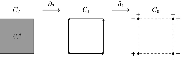
5.1 Boundary Operator . . . 63
5.1.1 Example:Boundary of a 1-rectangle . . . 65
5.1.2 Example:Boundary of a 3-rectangle . . . 65
5.2 Chains . . . 67
5.2.1 Example:Boundary of a boundary . . . 68
5.3 Stokes’ Theorem . . . 70
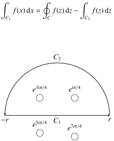
5.3.1 Example:Contour Integral . . . 73
6 Convolution of Piecewise Functions 76 6.1 Convolution of Piecewise Functions . . . 78
6.2 Hybrid Function Convolution . . . 81
6.2.1 Example:Hybrid Convolution . . . 82
6.3 Infinite Intervals . . . 84
6.4 Discrete Convolution . . . 85
6.5 Implementation . . . 87
7 Conclusions 91
Bibliography 93
A Convolution with Infinite End-Points 96
Curriculum Vitae 104
List of Figures
2.1 Piecewise Rational Function . . . 23
3.1 Possible block overlaps of 2×2 block matrices. . . 28
3.2 Cartesian product of two 1-rectangles . . . 34
4.1 Riemann Integral . . . 52
4.2 Approximations using simple functions . . . 55
5.1 Unit cube with boundary . . . 66
5.2 Orientations of 2-rectangles . . . 66
5.3 Boundary of a boundary (of a (2-)rectagle) . . . 68
5.4 Contour Integral . . . 74
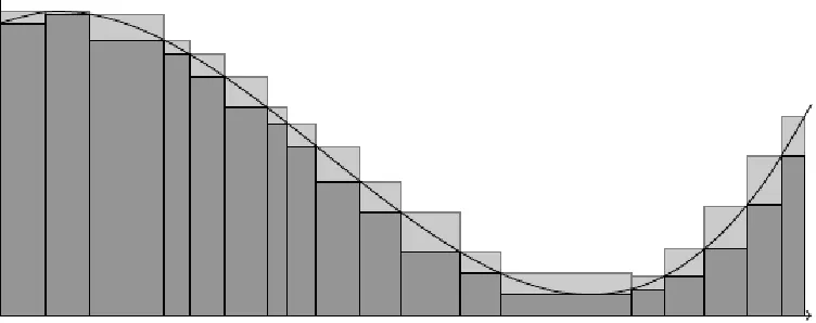
6.1 Convolution of box signal with itself . . . 76
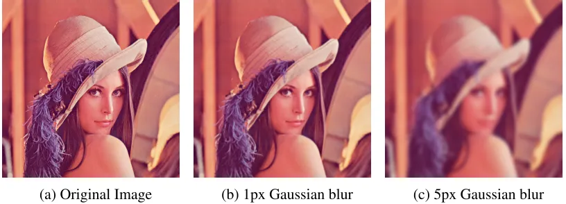
6.2 Gaussian Blurring . . . 77
6.3 Convolution of “one-piece” functions . . . 79
Introduction
1.1
Motivation
Some data structures in mathematics are more widely adopted than others and none more than
Cantor’s notion of sets. The very foundations of mathematics lie in set theory: numbers are
de-fined in terms of sets as are ordered tuples which in turn lead to relations, functions, sequences
and from there branches into countless other structures. But this trunk typically omits a
satis-factory treatment of severalgeneralized sets. For example, it is difficult to begin speaking about
hybrid setswithout immediately punctuating,“—that is, multi-sets with negative multiplicity”.
It is a statement of progress that multi-sets have even entered into common mathematical
parlance. On the other hand, sequences need no introduction and one can easily represent a
multi-set by a sequence: if an element occurs in a multi-set with multiplicityn, ensure that it’s
in the corresponding sequencentimes as well. In this way, sequences are often usedin place
of multi-sets with the added structure of an ordering. Indeed,“why not?”, even if the order of
elements is not needed,“surely it can’t hurt?”
Consider theFundamental Theorem of Arithmetic:
“Every positive integer, except 1, is a product of primes. (. . . ) The standard form
ofnis unique; apart from rearrangement of factors,ncan be expressed as a product
of primes in one way only.” (Hardy and Wright 1979, p.2-3)
By recognizing the possibility of rearranging factors, the authors implicitly define the “product
2 Chapter1. Introduction
of primes” as a sequence rather than, more aptly a multi-set. For iterated, commutative
op-erators (e.g. P,Q,T,S
), the order of terms is irrelevant so then, “why order terms to begin
with?”Reisig [16] uses multi-sets to define relation nets where “. . . several individuals of some
sort do not have to be distinguished", and moreover “Oneshould notbe forced to distinguish
individuals if one doesn’t wish to. This would lead to overspecification” (emphasis added).
The same applies here.
Next — and this is a more subtle and subjective point — the empty sequence is not nearly
as enshrined as the empty set. Whereas the empty set is often the first thing that comes to
mind when searching for trivial cases or counter-examples, the empty sequence is not usually
so readily recalled. Despite the empty sequence being just as well-defined as the empty set; it
tends to be treated as an aberrant case. In the case of iterated operators over an empty set, it
is simply the respective identity. In the case of Q
, this is 1, and so 1is a product of primes.
It is uniquely, the product of the empty set of primes. Similarly, a sequence containing just
one element is still a sequence but this also can be easy to forget. Some definitions will also
disregard this to say, “is prime or the product of primes”. Whether this is extra specificity is a
fault to the authors or simply a reminder to readers, the point remains the same. The perception
of sequences can be misleading in ways in which sets are not often misconstrued. Stripped of
these qualifications we are left with the more succinct:
“Every positive integer is the product of a unique multiset of primes.”
It goes deeper than a matter of aesthetics. Sets are certainly flexible objects and it is
tempt-ing to take a minimal approach to the tools required in one’s toolbox. But the algebra of sets,
is a fairly restrictive one. Consider the sets [a,b)={x|a≤ x <b}and [b,c)= {x|b ≤ x< c}.
Their union [a,b)∪[b,c) will depend heavily on the relative ordering ofa,bandc. More often,
as in integration what one really wants is “[a,b)+[b,c) = [a,c)”. When Boolean algebra and
numeric algebra interface, results can get unnecessarily messy. Hybrid sets will allow us to
remove this tension, by committing fully to numeric algebra. In this spirit that we will graft
1.2
Objectives
This thesis will include and extend the work of [7] on hybrid sets and their applications. In
particular we will take as inspiration from two famous identities. Consider the union of two
setsAand B. To compute the cardinality, one approach would be to partition the set into three
pieces: (A\B), (B\A) and (A∩B). The union, as the disjoint union of these three sets is then
the sum of their cardinalities:
|A∪B|=|A\B|+|B\A|+|A∩B|
The more common approach is to use the principle of inclusion-exclusion and instead break
A∪Binto the piecesA, Band (A∩B):
|A∪B|=|A|+|B| − |A∩B| (1.1)
Unlike the first approach, we no longer have a partition ofA∪Bin the traditional sense of the
term but in many ways, it still behaves like one.
Our other inspiration comes from integration where it is commonly defined that
Z b a
f(x) dx=−
Z a b
f(x) dx (1.2)
This allows for, regardless of the ordering ofa,bandc:
Z c a
f(x) dx=
Z b a
f(x) dx+
Z c b
f(x) dx
One can think of the region from a to c being partitioned into a tob and b to c. But again,
this is not a partition in the usual sense. Rather than a union of disjoint subsets, we again use
a generalized notion of a partition with sum oforientedsubsets where we can exclude subsets
4 Chapter1. Introduction
Reversed intervals within integration are not generally regarded any differently. Inclusion
and exclusion, are simply a matter of orientation. On the other hand, when excluding sets,
inverted elements are not usually regarded as objects of their own; “−(A∩B)” is not a set.
We will consider several different applications. When matrices are represented in terms of
block submatrices, the sum or product can vary depending on operand block sizes.
Represent-ing the regions of a block matrix with hybrid sets will allow for all cases to be consolidated
into one; no matter how those blocks may overlap. Lebesgue integration relies on measurable
sets and also does not naturally support orientation. Here, hybrid sets will allow us to evaluate
integrals like R0
1 1R\Qdx = −1 Finally, we will consider the convolution of piecewise interval
functions. Typically different equations are used depending on the relative length of intervals
but with hybrid sets we can condense this into one general equation and ignore the interval
lengths altogether.
Unifying all of this is the argument that hybrid sets are a very useful structure and there are
many instances where existing structures ought to be replaced. Hopefully these examples will
provide inspiration to the reader to recognize similar situations elsewhere as well.
1.3
Related Work
It is difficult to date the origin of multisets. Although the term itself was coined by De Bruijn
in corresponces with Knuth [13], the thought of a “collection of objects that may or may not
be distinguished” is as old as tally marks. In regards to the generalization tosignedmultisets,
Hailperin [12] suggests that Boole’s 1854Laws of Thought[6] is actually a treatise of signed
multisets. Whether this was Boole’s intent is debateable. Sets with negative membership
explicitly began to appear in [23] and were formalized under the name Hybrid sets in Blizard’s
extensive work with generalized sets [4, 5] Although hybrid set and signed multiset are the
most common nomenclature, other names appearing in literature include multiset (specifying
Existing explicit applications of hybrid sets are currently limited. Loebet al. [1, 15] use
hybrid sets to generalize several combinatoric identities to negative values. Bailey et al. [2]
and Banâtreet al. [3] have also had success with hybrid sets in chemical programming.
Repre-senting a solution is represented as a collection of atoms and molecules, negative multiplicities
are treated as “antimatter” . For a deeper overview and systemization of generalized sets, see
[18, 20]. These ideas allow symbolic computation on functions defined piecewise [7].
1.4
Thesis Outline
In Chapter 2, the foundations for hybrid sets and functions with hybrid set domains will be
laid. This will provide us with formal definitions and some immediate applications to
piece-wise functions will be presented. Chapter 3 will see hybrid domains applied towards symbolic
matrix algebra. Addition has already been considered [7], but this will be extended to
multipli-cation as well. In Chapter 4, hybrid functions will be applied towards integration. We will start
from foundations and use hybrid functions to allow for an oriented Lebesgue integral. We will
then show how hybrid sets naturally come up in Stokes’ theorem with the boundary operator.
Chapter 2
Hybrid Set Theory
The motivation behind hybrid sets and functions can be traced to wanting a better approach to
piecewise functions and closely related to that is a more generalized notion of a partition. In
general, we assume a piecewise function f : P→ Xwill take the form:
f(x)=
f1(x) x∈P1
f2(x) x∈P2
... ...
fn(x) x∈Pn
(2.1)
where the set {Pi} is a partition of P, the domain of f. and each function fi : Pi → X is
defined over a corresponding part ofP. We assume that fiis fully defined onPi(total) but may
be partial on P. Frequently these partitions are not expressed explicitly as sets but rather as
conditions. For example, the absolute value function is far more commonly written out as
abs(x)=
−x x<0
x x≥0
rather than abs(x)=
−x {x|x∈R∧x< 0}
x {x|x∈R∧x≥ 0}
but using conditions rather than the sets they define can be seen as just a shorthand.
One thing that should be noted is that sometimes there are additional conjuncts bundled
into a condition. As pieces of a partition, the sets generated must be disjoint so we must ensure
these conditions are mutually exclusive. A common heuristic is to treat these conditions as a
series of cascadingelse-if statements. For exampleMaple’spiecewisefunction:
piecewise(cond_1, f_1, cond_2, f_2, ..., cond_n, f_n, f_otherwise)
will evaluate eachcond_1 in order and when one evaluates to true, the corresponding f_iis
then evaluated. Finally if all ofcond_ievaluate to false thenf_otherwiseis used. Hence the
partitions corresponding to eachcond_iis notjust{x | cond_i(x)}but instead the set where
cond_iis true andall precedingconditions are also false.
Although the notation used in (2.1) is fine for piecewise functions with only a few terms
such as abs, it quickly becomes unwieldy when one wants to add more pieces. So instead we
will use thejoinof disjoint functionrestrictions.
Definition Given a function f : X → Y and any subset of the domain Z ⊂ X, therestriction
of f toZis the function f|Z :Z →Y, such that f|Z(x)= f(x) for allx∈Z.
There are several ways which one could define a join operator; specifically how one deals
with intersections. One could favor the first function as Maple does, but we will take the stance
that the intersection is poorly defined.
Definition Define, thejoinof two functions, f andgby:
f g=
f(x) ifg(x)=⊥
g(x) if f(x)=⊥
⊥ otherwise
(2.2)
Where the bottom element⊥denotes that the function is undefined. As such if f :X →Y and
8 Chapter2. HybridSetTheory
difference. Together these definitions allow us to re-write the piecewise function in (2.1) as:
f = f|P
1 f|P2 . . . f|Pn
Normally, the join operator is not associative and so omitting parentheses could lead to
poorly defined expressions. However, when all support sets are pairwise disjoint, then is
associative.
Now consider arithmetic of two piecewise functions. Let f andgbe two piecewise
func-tions f = f1|P1 f2|P2 f3|P3
andg = g1|Q1 g2|Q2
. To compute the sum f +gwe need
to consider each possible intersection of partitions of P and partitions ofQ. In this case, the
result is generally a piecewise function with 6 terms:
(f +g)= (f1+g1)|P1∩Q1 (f1+g2)|P1∩Q2 (f1+g3)|P1∩Q3
(f2+g1)|P2∩Q1 (f2+g2)|P2∩Q2 (f2+g3)|P2∩Q3
In specific cases, some terms may be eliminated as the corresponding intersection is empty. In
general, assuming no degenerate intersections, the sum of an “n-piece” function and “m-piece”
function will give a piecewise function with n· m pieces. This becomes compounded when
dealing with more piecewise functions. The sum ofbfunctions each withnpieces results inbn
cases making computation unrealistic in all but the smallest cases.
Another perspective to take is to first find acommon refinementofP={Pi}i∈IandQ={Qj}j∈J.
In the above example we selected the refinement:
R= n(P1∩Q1), (P2∩Q1), (P3∩Q1), (P1∩Q2), (P2∩Q2), (P3∩Q2)
o
That is, for each Pi in the partition P, there is a subset of R which will partition Pi (namely
Pi = {(Pi∩Q1),(Pi∩Q2)}and soRis a refinementof P. SimilarlyRalso a refinement of Q
Finding common refinements gives a large increase in the number of terms required, in
part, due to a restrictive view of partitions. Conceptually, what one wishes out of a partition is
a family of subsets which will “sum” up to the original. With Boolean sets, some additional
constraints are imposed as we don’t have a very good notion of subtraction. However, with
more general structures, we can construct true inverse sets to allow for algebraic cancellations.
Following the development of [7], over this chapter we will consider such generalized partitions
and the structures to support them. We will also see how this allows for us to eliminate the
multiplicative increase in terms when flattening an expression containing the sum or product
of piecewise functions.
2.1
Hybrid Sets
We considerhybrid setswhich are a generalization of multi-sets. One can view usual Boolean
sets as an indicator function on the universe which maps each member element to 1 and each
non-member to 0. Amulti-set (orbag) extends this by allowing multiple copies of the same
element. The indicator function of a multi-set would therefore range overN0, the set of
non-negative integers. Hybrid sets take this one step further allowing for an element to occur
negatively manytimes as an indicator function over the integers.
Definition LetU be a set, then any functionU → Zis called a hybrid set. We denote the
collection of all hybrid sets over an underlining setU byZU.
This provides a functional back-end for constructing hybrid sets. However, given the name,
we would like our hybrid sets to at least resemble sets. So we introduce the following
defini-tions to better interface with the underlying integer funcdefini-tions.
Definition Let H be a hybrid set. Then we say that H(x) is the multiplicity of the element
x. We write, x ∈n H if H(x) = n. Furthermore we will use x ∈ H to denote H(x)
, 0 (or
equivalently, x∈n Hforn
10 Chapter2. HybridSetTheory
will be used to denote the empty hybrid set for which all elements have multiplicity 0. Finally
thesupport of a hybrid setis the (non-hybrid) set supp H, where x ∈ supp H if and only if
x∈H
We will use the notation:
H =n
x
m1
1 ,x
m2
2 , . . .
o
to describe the hybrid setHwhere the elementxi has multiplicitymi. We allow for repetitions
in{xi}but interpret the overall multiplicity of an elementxi as the sum of multiplicities among
copies. For example, H = n a
1,a1,b−2,a3,b1 o
= n
a
5,b−1 o
. The latter will generally be
preferred as alla’s andb’s have been collected together. Such a writing in whichxi , xjfor all
i, jis referred to as anormalized formof a hybrid set.
Boolean sets use the operations ∪ union, ∩ intersection, and \ complementation. These
correspond to the Boolean point-wise∨OR,∧AND, and¬NOToperations. That is, for two sets
A andB, then (A∪B)(x) = A(x)∨B(x). Onecouldextend these for hybrid sets using
point-wise min and max on multiplicities as in [4, 5, 11, 19] but this is not very natural. Rather, our
primitive hybrid set operations should derive from our primitive point-wise operators. When
dealing with hybrid sets with multiplicities over the integers, we have the ring (Z,+,×). Thus
we will define⊕, , and⊗by point-wise+,−, and×respectively.
Definition For any two hybrid setsAandBover a common universeU, we define the
opera-tions⊕, ,⊗ :ZU ×ZU →ZU such that for allx∈U:
(A⊕B)(x)= A(x)+B(x) (2.3)
(A B)(x)= A(x)−B(x) (2.4)
(A⊗B)(x)= A(x)·B(x) (2.5)
We also define, Aas∅ Aand forc∈Z:
Definition We say AandBare disjointif and only ifA⊗B=∅
For Boolean sets Aand B, disjointness would be defined by A∩B = ∅. If we consider these
Boolean sets as simply hybrid sets with multiplicity 0 or 1 then the operations∩and⊗
identi-cally correspond to element-wiseAND.
From these definitions, we can use hybrid sets to model various objects that would
tradi-tionally be described otherwise. For example, any positive rational number can be represented
as a hybrid set over the primes.
(ZP,⊕)'(Q+,×)
For a positive rational numbera/b, bothaandbbeing integers will have a prime
decomposi-tion: a = (pm1
1 · p
m2
2 ·. . .) andb = (q
n1
1 ·q
n2
2 ·. . .) then there is the group isomorphism f given
by:
f(a/b)= n p
m1
1 ,p
m2
2 , . . .
o n
q
n1
1 ,q
n2
2 , . . .
o
Furthermore, we have the equivalence ca/cb = a/b for free by writing the hybrid set in
nor-malized form (e.g. 2/4 = n 2
1,2−2 o
= n
2
−1 o
= 1/2). One could also think of the roots and
asymptotes of a rational polynomial as a hybrid set over the underlying ring:
(x−2)
(x−1)2(x+1) =
n 2
1,1−2,−1−1 o
Depending on the context, a negative multiplicity could take many different meanings. Rather
than attach a single rigid concept, we will keep this flexibly abstract sometimes. In these
examples we used the multiplicity as an exponent in other cases it is more aptly a coefficient
or as orientation.
All Boolean sets can be trivially converted to hybrid sets. For a setX, this is done simply by
takingH(x)= 1 ifx∈X andH(x)=0 if x<X. We will often perform this conversion silently
by applying hybrid set operators to Boolean sets. The reverse conversion: the reduction of a
12 Chapter2. HybridSetTheory
Definition Given a hybrid setH over universeU, if for all x ∈U H(x) = 1 or H(x) = 0 then
we say that H(x) is reducible. IfH is reducible then we denote thereduction of H byR(H)
as the (non-hybrid) set overU with the same membership.
In Boolean set theory, a partition ofXis a collection of subsets ofXsuch thatXis a disjoint
union of the subsets. When dealing with hybrid sets we no longer have (or rather choose not to
use) union but use point-wise sum instead. For disjoint, reducible hybrid sets, point-wise sum
and union agree but we will be even more accommodating and allow for any family of sets
which sum to a hybrid set to be a (generalized) partition.
Definition Ageneralized partitionPof a hybrid setH(x)is a family of hybrid setsP= {Pi}ni=1
such that:
H = P1⊕P2⊕. . .⊕Pn (2.7)
We say that Pis a strict partition ofHifPi andPj are disjoint wheni, j.
If a setHis reducible, then strict generalized partitions will correspond to the usual notion
of a partition. A traditional partition will be a disjoint cover of H and for disjoint reducible
sets, point-wise sum and union agree. HenceS
iPi =
L
iPi. Conversely, ifH is reducible and
the sum of disjoint hybrid sets, thenPi must all be reducible as well.
This does not hold for a non-strict partition of a reducible hybrid set. Consider the interval
[0,1] as a hybrid set (that is, H(x) = 1 if 0 ≤ x ≤ 1 and H(x) = 0 otherwise). Then P =
[0,2], (1,
2] is a generalized partition of H. A generalized partition of a reducible set is
strict if and only if each generalized partition is reducible.
2.2
Hybrid Functions
A function is typically defined as a mapping from elements of one set to another set. We
which we will call hybrid functions. We will define hybrid functions as the collection of all
pairs (x, f(x)) (i.e. thegraph of the function f).
Definition For two setsS andT, a hybrid set over their Cartesian product S × T is called a
hybrid (binary) relation between S and T. We denote the set of all such hybrid relations
by ZS×T. A hybrid function fromS toT is a hybrid relation H betweenS andT such that
(x,y)∈Hand (x,z)∈Himpliesy=z. We denote the set of all such hybrid functions byZS→T.
Again we will need some notation for this to be more usable. We would like to think of a
hybrid function not as a mapping from a hybrid set to a Boolean set but rather as a function
between two Boolean sets and integer multiplicity attached to the mapping (the “arrow” itself).
In this way we partially separate the traditional function and the multiplicity function (given as
a hybrid set) and view a hybrid function as their combined object. Formally, given a hybrid set
H overU and a function f : B → S be a function where B ⊆ U andS a set. Then we denote
by fHthe hybrid function fromBtoS defined by:
fH:= M
x∈B
H(x)n
(x, f(x))
1 o
(2.8)
There is little literature or established use for hybrid functions; their primary use to us will
be as something that we can turn back into traditional functions. So as with hybrid sets, we
would like a notion of reducibility.
Definition IfH is a reducible hybrid set, then fH is a reducible hybrid function.
Addition-ally, if fHis reducible, we extendRby:
R(fH)(x)= f|R(H)(x) (2.9)
Since R(H) only exists if H(x) is everywhere 0 or 1; R(fH) only makes sense when fH
is reducible. Assuming that we end up with a reducible function, hybrid functions will make
14 Chapter2. HybridSetTheory
to construct piecewise functions from restricted functions. The join operator for two hybrid
functions is quite trivially defined.
Definition Thejoin, fF gG of two hybrid functions fF andgG is the hybrid relation given
by their point-wise sum.
fFgG= fF ⊕gG (2.10)
However, we will immediately dispense with usingaltogether and simply use⊕in order
to prevent confusion between hybrid functional join (e.g. fF ⊕gG) and traditional functional
join (e.g. f|Fg|G). It is important to note that the join operator is closed under hybrid relations
but not under hybrid functions. For any two hybridfunctionsthe result will be a hybridrelation
but not necessarily another hybrid function. As with traditional functional join, we must still
be wary of overlapping regions but non-disjoint hybrid domains are not nearly as “dangerous”.
For intersecting regions we do not have to choose between commutativity and associativity, we
can have both. In general, all that we can say the result is a hybrid relation but there are many
cases where we can guarantee hybrid function status is preserved.
Lemma 2.2.1 Let A and B be hybrid sets over U and let f : U → S be a function. Then
fA⊕ fBis a hybrid function. Moreover,
fA⊕ fB = fA⊕B (2.11)
Proof Since fA and fB are hybrid functions with a common underlying function f, all
ele-ments with non-zero multiplicity in either set will be of the form (x, f(x)). As there can be
no disagreement between among points for a common function, the pointwise sum must be a
hybrid function. For x ∈ U, we have x ∈n Aand x ∈m Bfor some (possibly zero) integersm
andn. Hence, (x, f(x)) ∈m fA and (x, f(x)) ∈n fB and (x, f(x)) ∈(m+n) (fA⊕ fB). At the same
Joining a function with itself is not the most interesting construction. Generally piecewise
function is desired for it’s ability to tie together twodifferent functions. If two functions have
separate, non-overlapping regions, then our definition is again trivial.
Lemma 2.2.2 Given two function f :U → S and g : U →S . The following identity holds if
and only if A and B are disjoint:
fA⊕gB =(f|suppAg|suppB)A⊕B (2.12)
Notice here the use of on the right hand side. Here is the traditional (non-hybrid)
function join as defined in (2.2). (f g) was undefined for supp(A)∩supp(B)
and so the
equality will not hold if A and B are not disjoint. Chaining several sums together we can
represent the piecewise function f from (2.1) by:
fP = fP1 ⊕ fP2 ⊕. . .⊕ fPn
Proof Again, as hybrid functions, all elements with non-zero multiplicity of fA and gB will
be of the forms (x, f(x)) or (x,g(x)) respectively. Suppose that we have (x, f(x)) ∈n fA and
(x,g(x)) ∈m gB for disjoint A and B. Ifn , 0, then we have m = 0 as disjointness implies
A⊗B= ∅and so A(x)·B(x)= m·n= 0. Similarly ifm, 0 thenn=0. Thus if (x, f(x))∈ fA
then (x,g(x))<gB and vice versa and so fA⊕gBis a hybrid function.
We can then safely construct (f|suppAg|suppB) without undefined points as suppA∩suppB=
∅. For (x, f(x)) ∈m (fA ⊕gB) with non-zerom, we have (f|suppA g|suppB)(x)= f(x) andx ∈m
A⊕B. Similarly for (x,g(x))∈n (fA⊕gB) with non-zeron, we have (f|suppAg|suppB)(x)=g(x)
andx∈n
A⊕B. Thus, fA⊕gB =(f|suppA g|suppB)A⊕B.
But disjointness is still too strong of a condition for two hybrid functions to be compatible.
The join of two non-disjoint functions may still be a hybrid function even if their respective
16 Chapter2. HybridSetTheory
Theorem 2.2.3 For hybrid functions fA and gB, fA ⊕gBis a hybrid function if and only if for
all x∈supp(A⊗B), we have f(x)=g(x). We say that fA and gB are compatible.
Proof This follows from the preceeding two lemmas. For x ∈ supp(A⊗ B), if f(x) = g(x)
then we are simply combining two identical functions as in lemma 2.2.1. On the other hand
forx<supp(A⊗B) then either one or both ofA(x) orB(x) are zero. In this case we use lemma
2.2.2.
Compatibility becomes less clear when we begin to consider multiple hybrid functions. For
one, compatibility is not associative. Consider the following sequence:
(fH⊕gH)⊕g H = fH⊕(gH⊕g H)= fH⊕g∅ = fH
We know nothing of the compatibility of fH andgH but let us assume that they are not
com-patible. However even though (fH ⊕gH) is a hybrid relation it is compatible withg H. On the
other hand,gH andg Hare clearly compatible as an instance of theorem 2.2.1. The result is a
function over the empty setg∅which is compatible withanyhybrid function.
2.3
Hybrid Functional Fold
Compatibility and reducibility are one way of collapsing a hybrid function to a traditional
function. Another approach is to fold or aggregate a hybrid function using some operator. To
aid in this we will first introduce some notation for iterated operators.
Definition Let∗ :S×S → S be an operator onS. Then, forn>0,n∈Zwe use∗n:S×S →
S to denote iterated∗. So,
x∗ny= (((x
ntimes
z }| {
∗y)∗y)∗. . .∗y) (2.13)
If∗has an identitye∗, then we extend x∗0y= x. Ifyhas inversezunder∗then we usex∗−1y
to denotex∗1zand extend this for any naturalnby x∗−nybyx∗nz. Finally, we allow∗nto be
a unary operator, which we define by∗nx= e
Assuming∗mand∗n are both defined (e.g. ifm,n ≤ 0 then∗ must be invertible), we have
(x∗my)∗ny= x∗m+ny. For non-associative groupoids, it may be of interest to instead define∗T
for some treeT. For example∗n
above is analogous to Haskell’sfoldl. There are applications
wherefoldr: (x∗(y∗(y∗. . .∗y))) or a balanced expression tree likefoldtmight be desired.
The applications we will be interested in will be over associative group operators and so we
will not actually explore this any further.
Definition We say that a hybrid relation fA = fA1
1 ⊕f
A2
2 ⊕. . .overT×S is∗-reducibleif (S,∗)
is an abelian semi-group andAis everywhere non-negative or if (S,∗) is an abelian group, we
allow for for negative A. If fA is∗-reducible we define its∗-reduction, R∗(fA) : T → S as a
(non-hybrid) function:
R∗(fA)(x)=
∗A1(x)f
1(x)∗A2(x) f2(x)∗. . .
suppA (2.14)
If fA is reducible then it is trivially∗-reducible and we have:
R(fA)=R∗(fA) (2.15)
If a hybrid function is already “flattened”, then reducing it will do nothing. So clearlyR∗is a
projection since it is idempotent (i.e.R∗(R∗(fA))= R∗(fA)). Moreover, we can pull restrictions
through point-wise sums:
R∗(R∗(fF)⊕ R∗(gG))= R∗(fF ⊕gG) (2.16)
2.3.1
Example:
Piecewise functions on generalized partitions
LetA1= [0,a), A2= [0,1]\A1,B1 =[0,b) andB2= [0,1]\B1witha,b∈[0,1]. {A1,A2}and
18 Chapter2. HybridSetTheory
functions f andgwhich map to some group f,g: [0,1]→G.
f(x)= fA1
1 ⊕ f
A2
2 =
f1(x) x∈A1
f2(x) x∈A2
and g(x)=gB1
1 ⊕g
B2
2 =
g1(x) x∈ B1
g2(x) x∈ B2
If one were interested in computing their sum, (f + g), the naive method would be to
compute every possible intersection. Over each intersection, one then takes the restriction of
the corresponding sub-functions and joins all these terms together. As in,
(f +g)(x)= (f1+g1)|A1∩B1 (f1+g2)|A1∩B2 (f2+g1)|A2∩B1 (f2+g2)|A2∩B2
We will take another approach. First, we can partition [0,1] into the generalized partition
A1, B1 A1, B2. The source of this particular partition will remain mysterious for now but
observe that we can still construct the partitions: B1= (B1 A1)⊕A1andA2= (B1 A1)⊕B2.
And so we can represent f andgfrom above with a common partition by using:
f = fA1
1 ⊕ f
(B1 A1)⊕B2
2 = f
A1
1 ⊕ f
B1 A1
2 ⊕ f
B2
2
g=gA1⊕(B1 A1)
1 ⊕ g
B2
2 = g
A1
1 ⊕ g
B1 A1
1 ⊕ g
B2
2
Since we have a common partition we can avoid computing pairwise intersections
alto-gether and simply add each sub-function to the corresponding sub-function which shares a
partition. Since {A1,B1,(B1 A1)} is a generalized partition, we will need to flatten the
ex-pression back down to get a traditional function. We use R+ for this so that negative regions
properly cancel.
(f +g)(x)= R+(f1+g1)A1 ⊕(f2+g1)B1 A1 ⊕(f2+g2)B2
This equation holds regardless of the relative ordering of a and b. Suppose x ∈ A1∩B1
Similarly, if x ∈ B1∩A2 or x ∈ A2 ∩B2 then only (B1 A1)(x) or B2(x) will respectively be
non-zero. However, ifx ∈ B2∩A1then we haveA1(x) = 1, (B1 A1)(x)= −1 andB2(x) = 1.
Simplifying this expression yields:
(f +g) = +1(f1+g1)+−1(f2+g1)+1(f2+g2) = (f1+g2)
In the above example only three regions could simultaneously exist. Ifa<bthenA1∩B2 =
∅but if b < a thenA2 ∩B1 = ∅. Although it might seem that the three terms are a result of
three regions, in the general case whereA1andB1could be arbitrary subsets, we still only have
three terms. We will even extend this to any generalized partition. First we will formalize some
ideas we have already seen.
Definition Arefinementof a generalized partitionP={Pi}i∈I is another generalized partition
Q = {Qj}j∈J such that, for every Pi inP there is a subset of Q: {Qj}j∈Ji, Ji ⊆ J such that for
some integers{ai j}j∈Ji
Pi =
M
j∈Ji
ai jQj (2.17)
Given asetof generalized partitions acommon refinementis a generalized partition which is
a refinement of every partition in the set. A refinementQofPisstrictif supp(Q)=supp(P).
In our previous example we used{A1,B1 A1,B2}which was a common refinement of both
{A1,A2}and {B1,B2}. A1 and B2 have trivial representations while A2 = (B1 A1)⊕ B2 and
B1 = A1⊕(B1 A1). Another common refinement would be the trivial{A1,B1,A2,B2}This is
less preferable due to not only containing 4 regions instead of 3 but also the point-wise sum is
[0,1]2 instead of the reducible [0,1].
We can now formally phrase the problem. Let A = {Ai}ni=1 and B = {Bi}mi=1 be two
gener-alized partitions of a hybrid setU. We wish to find a generalized partitionC ofU which is a
20 Chapter2. HybridSetTheory
summarized into the following system ofn+m+1 simultaneous equations:
U = M
j
Cj
∀i∈1. . .n: Ai =
M
j
ai,jCj
∀i∈1. . .m: Bi =
M
j
bi,jCj
for some integersai,j and bi,j. Since we know that A and B are each separately partitions of
U, we can leverage some of their dependencies to construct {Cj}. For example, An can be
represented asU (A1⊕. . .⊕An−1). AnyAiorBi could similarly be represented by the
point-wise difference with U. Although we could remove any two pieces from A and B, we will
choose to remove An and Bn to form a set of n+m−1 pieces to form a linearly independent
basis forC. Expressed as a linear system we have:
M· C1 ... Cn+m−1
= U A1 ... An−1
B1
... Bm−1
where M =
1 1 · · · 1
a1,1 a1,2 · · · a1,n+m−1
... ...
an−1,1 an−1,2 · · · an−1,n+m−1
b1,1 b1,2 · · · b1,n+m−1
... ...
bm−1,1 bm−1,2 · · · bm−1,n+m−1
By definition,Mis an integer matrix. But we are actually more interested in its inverseM−1
as this will give us values forCirelative to (U,A1, . . . ,Am−1,B1, . . . ,Bm−1). To stay in the realm
of hybrid sets, we would also like to enforce that M−1 is also an integer matrix. Assuming
this, then the determinant of M must be±1. Further restricting ourselves to upper triangular
the following inverse:
1 · · · 1
0 1 0 · · · 0 ... ... ... ... ... ... ... ... 0 0 · · · 0 1
−1 =
1 −1 · · · −1
0 1 0 · · · 0 ... ... ... ... ... ... ... ... 0 0 · · · 0 1
Using this, we find that one choice forCthe common refinement forAandB, is:
C =n(U A1 . . . An−1 B1 . . . Bn−1), A1,A2, . . . ,An−1, B1,B2, . . . ,Bm−1
o
Finally, to generalize the example from 2.3.1, let f = fA1
1 ⊕ f
A2
2 ⊕ f
An
n andg=g B1
1 ⊕. . .⊕g
Bm
m
be two piecewise functions over a common domainU. We can express both of these functions
in terms of the above common refinement by:
f = fA1
1 ⊕. . .⊕ f
An−1
n−1 ⊕ f
U⊕B1⊕...⊕Bm−1
n
g= gB1
1 ⊕. . .⊕g
Bm−1
m−1 ⊕g
U⊕A1⊕...⊕An−1
m
To compute (f ∗g) one just needs to collect like terms and encapsulate in a∗-reduction
f ∗g= R∗
(f1∗gm)A1 ⊕. . .⊕(fn−1∗gm)An−1
⊕(fn∗g1)B1 ⊕. . .⊕(fn∗gm−1)Bm−1 (2.18)
⊕(fn∗gm)U (A1
⊕...⊕An−1⊕B1⊕...⊕Bm−1)
2.4
Pseudo-functions
One last detail remains to be settled. So far we have assumed that the sub-functions of f andg
22 Chapter2. HybridSetTheory
be defined over its corresponding partAiand similarlygj overBj. This poses a problem for the
previous equation (2.18) when evaluated at sayx∈A1∩B1. Then we have the following terms
with non-zero multiplicity:
(f ∗g)(x)=R∗
(f1(x)∗gm(x))1⊕(fn(x)∗g1(x))1⊕(fn(x)∗gm(x))−1
We would like for the gm(x) in the first term to cancel with the gm(x) in the third term.
Similarly fn(x) in the second term should cancel with the fn(x) in the third term leaving only
f1(x)∗g1(x). This requires thatgm(x) and fn(x) to actually be defined which is more than we’d
care to assume. The approach we take instead is to delay the evaluation of functions until
cancellations occur. To do this we use a lambda-lifting trick. Instead of having the elements
of a hybrid function be pairs containing the input and output of the underlying function we
consider them as pairs containing the input and a “function pointer” to the underlying function.
Definition We define a pseudo-function ef
A as:
ef
A
= M
x∈B
A(x)n
(x, f)
1 o
(2.19)
One should notice the similarity between (2.19) and (2.8). The difference is that we have
replaced (x, f(x)) with the unevaluated (x, f). This formally makes ef
A
a hybrid relation over
U×(U → S) as opposed to a hybrid function overU×S. To evaluateef
A
we map back to fAand
evaluate that. This mapping between (x, f(x)) and (x, f) is very natural and we will perform it
unceremoniously, often using fA and
ef
A
interchangeably. Properties of hybrid functions such
2.4.1
Example:
Piecewise functions revisited
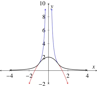
We repeat the example from 2.3.1 but concretely use the following function:
f(x)=
(2− x2) −1≤ x≤1
1/x2 otherwise
Graphically, this resembles a bell-shaped curve with no discontinuities or any apparent
irregu-lar behavior. This can be seen in the black plot below in Figure 2.1. Although f is defined for
all ofR, this is not the case for its sub-functions. The plots in red and blue show the behavior
of (2−x2) and 1/x2 respectively outside of their defined ranges in f. Of note, 1/x2 (shown in
blue) is obviously undefined at 0.
−4 −2 2 4
−2 2 4 6 8 10
x y
Figure 2.1: A piecewise rational function is shown in black. The plots in red and blue are continuations of (2− x2) and 1/x2respectively.
To represent f as a hybrid function, we partition the real line into the sets A1= [−1,1] and
A2 = R\[−1,1] = (−∞,−1)⊕ (1,∞). This gives the closely related hybrid function f and
pseudo-function ef :
f = 2−x2A1 ⊕ 1/x2A2
ef =
24 Chapter2. HybridSetTheory
Additionally we will multiply f by the Heaviside functionH: a piecewise function over the
intervalsB1 =[0,∞) andB2 =(−∞,0) defined as follows:
H = (1)B1 ⊕ (0)B2
e
H = (x7→1)B1 ⊕ (x7→0)B2
In both the pseudo and non-pseudo function cases, we first need to find a minimal common
refinement. As before, we can construct the common refinementP= {P1,P2,P3}:
P1 = A1 = [−1,1]
P2 = B1 = [0,∞)
P3 = U (A1⊕B1) = R [−1,1] [0,∞)
To illustrate the problem with using (non-pseudo) hybrid functions, we shall consider f · H
evaluated at 0. Since f(0)= 2 and H(0) =1 we expect (f ·H)(0)= 2. Following from (2.18),
we construct a hybrid function andattempt:
(f ×H)(0)= R×
(2−x2)(0)P1 ⊕(1/x2)(1)P2 ⊕(1/x2)(0)P3
(0)
= R×
(2−02)(0)1⊕(1/02)(1)1⊕(1/02)(0)−1
= (2−02)(0)·(1)(1)·(02)(1)
(1)(1)·(02)(1)·(1)(0)
But it is not so easy to argue that this evaluates to 2. Alternatively, we could use the very
similar pseudo-function:
ef ·He=R×
(x7→ 2−x2)·(x7→0)P1
⊕ (x7→ 1/x2)·(x7→1)P2
⊕ (x7→ 1/x2)·(x7→0)P3
Leaving these functions unevaluated is the key to making non-total functions work. Once
again, we evaluate each ofP1, P2andP3at 0 and find:
(ef ·H)(0)e = R×
(x7→2− x2)·(x7→0)1
⊕ (x7→1/x2)·(x7→1)1
⊕ (x7→1/x2)·(x7→0)−1
(0)
Once we have this, we can then evaluate the multiplication-reductionR×, on the still
unevalu-ated functions. Clearly x 7→ 0 occurs with canceling signs as does x 7→ 1/x2. This leaves us
with the product of two unevaluated functions:
(ef ·H)(0)e =
(x7→2−x2)·(x7→1)
Afterthese cancellations occur, then we can evaluate (f ·H)(x) by way of ((ef ·H)(x))(x):e
(f ·H)(0) = ef ·He
(0)(0) = (x7→ 2−x2)·(x7→1)(0) = 2
Aside from the introduction of R∗as a correction to the :∗operation, the material of this
chapter can be found entirely in [7]. Given this foundation, the following four chapters will
explore new applications for hybrid sets and functions. Matrix addition with block matrices
was also explored in [7] as well as [17]. In the following chapter these will be revisited and
extended. A novel technique for matrix multiplication will also be presented. The next obvious
application for hybrid sets is as oriented domain of integration. We will perform an otherwise
standard treatment of integration but for the new usage of hybrid sets and oriented intervals.
There are other ways to deal with orientation in Lebesgue integrals but hybrid sets will allow
us do so directly without the need to “sanitize” domains. Finally all of our work with integrals
and piecewise functions will culminate in chapter 6 with a novel approach to convolution of
Chapter 3
Symbolic Block Linear Algebra
In mathematics literature, it is common practice to represent matrices as being broken up into
blocks or sub-matrices. For example ifA, B,C andDare matrices given by:
A=
A1,1 . . . A1,m ... ... An,1 . . . An,m
B=
B1,1 . . . B1,q ... ... Bn,1 . . . Bn,q
C =
C1,1 . . . C1,m ... ... Cr,1 . . . Cr,m
D=
D1,1 . . . D1,q ... ... Dr,1 . . . Dr,q
Where, critically,AandChave the same width (namelym) as doBandD(widthq).
Addition-ally,AandBhave the same height (in this casen), as doCandD(heightr). Then they can be
“glued” together into a single(2×2) block matrixM. Notationally, we write these matrices
as elements ofMbut weinterpret Mas a sort of concatenation of the sub-matrices.
M= A B C D =
A1,1 . . . A1,m B1,1 . . . B1,q
... ... ... ...
An,1 . . . An,m Bn,1 . . . Bn,q
C1,1 . . . C1,m D1,1 . . . D1,q
... ... ... ...
Cr,1 . . . Cr,m Dr,1 . . . Dr,q
So Mis actually a (n+r)×(m+q) matrix but we write it as a 2×2blockmatrix. Within
an individual block, there is a one-to-one correspondence from the entries of Mto the entries
of a sub-matrix (shifted by some offset). In the above example, elements ofBwould have an
offset of (0,m) sinceBi,j corresponds withMi+0,j+m.
There is no reason to stop at combining 4 matrices into a 2×2 block matrix. We can take
a set of matricesAi,j and combine them into an(n×m) block matrix:
M =
A1,1 A1,2 . . . A1,m
A2,1 A2,2 . . . A2,m ... ... ... An,1 An,2 . . . An,m
In the 2×2 case, we enforced that for example the height ofAwas the same as the height
ofB. Similarly, here it is an important condition that these partitions are divided byunbroken
horizontal and vertical lines. Formally, for each sub-matrixAi,j inMthenAi,jis a si×tjmatrix
for strictly positive integer sequences{si}ni=1 and{tj}mj=1 common to all sub-matrices. As before
we interpret the block matrix as a concatenation of its sub-matrices. Thus M is an×mblock
matrix but a Pn i=1si×
Pm
j=1tj
block matrix.
Clearly block matrices are at the very least a convenient notation but they also have
con-siderable practical applications as well. For example when multiplying large matrices, block
matrices can be used to improve cache complexity [14]. Additionally, in some cases, when a
sub-matrices are known to have a nice properties, many optimizations can arise. For example
to invert what is known as ablock diagonal matrix, one can invert each block individually:
A1 0 . . . 0
0 A2 ... ...
... ... ... 0 0 . . . 0 An
−1 =
A1−1 0 . . . 0
0 A2−1 ... ...
... ... ... 0 0 . . . 0 An−1
28 Chapter3. SymbolicBlockLinearAlgebra
(a)
" #
(b)
∗ ∗
(c)
"
∗ ∗
#
(d)
∗ ∗ ∗ ∗
∗
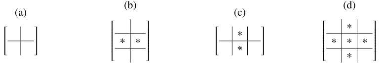
Figure 3.1: The sum of two block matrices each with four blocks leads to 9 possible cases. When blocks are exactly the same size, the sum will also be a 2×2 block matrix (a). Otherwise, a 2×3 (b)(two possible cases), 3×2 (c)(two cases)or 3×3 (d)(four cases)block matrix could arise. The starred blocks may sample from different blocks depending on the relative size of operand blocks.
Existing techniques allow for fixed block size but are unsatisfactory when the bounds
be-tween blocks are symbolic. For example, the sum of 2× 2 block matrices, naively leads to
9 possible cases of overlapping regions depending on the relationship between horizontal and
vertical boundaries between blocks. In this chapter we will show a method using hybrid
func-tions to avoid this case based approach for both addition and multiplication of matrices. First
we introduce some notation that will be used frequently over the next few chapters.
3.1
Oriented Intervals
Definition Given a totally ordered set (X,≤)(and with an implied strict ordering<), for any
a,b ∈ X, an interval between a and b is the set of elements in X between a and b, up to
inclusion ofaandbthemselves. Formally:
[a,b]X = {x∈X |a≤ x≤b}
[a,b)X = {x∈X |a≤ x<b}
(a,b]X = {x∈X |a< x≤b}
(a,b)X = {x∈X |a< x<b}
(3.3)
When context makesXobvious or the choice ofXis irrelevant, we shall omit the subscript.
It should be noted that whenbis less thana, [b,a] is the empty set. In terms of idempotency,
points equivalent toawhile (a,a), (a,a], and [a,a) are all empty sets. As intervals are simply
sets, they can naturally be interpreted as hybrid sets. Ifa ≤ b ≤ c, for intervals then we have
[a,b)⊕[b,c)= [a,c). In this case,⊕seems to behave like concatenation but this is not always
true. If instead we hada≤ c≤bthen [a,b)⊕[b,c)=[a,b).
[a,b)⊕[b,c)=
[a,c) a≤ b≤c
[a,b) a≤ c≤b
[b,c) b≤ a≤c
∅ otherwise
One could alternatively write [a,b)⊕[b,c)=[ min(a,b),max(b,c) ) but this simply sweeps
the problem under the rug. When working with intervals, a case-based approach to consider
relative ordering of endpoints easily becomes quite cumbersome. Previously, the ξ function
was introduced in [17] to solve this problem. Although it solves the problem of cases, it
quickly leads to unnecessarily heavy notation. Instead we introduce oriented intervals which
are considerably more readable. It should be noted that the definitions are equivalent;ξ(i,y,z)
and [[y,z)) can be used interchangeably.
Definition We defineoriented intervalswitha,b∈X, whereXis a totally ordered set, using
hybrid set point-wise subtraction as follows:
[[a,b))= [a,b) [b,a)
((a,b]]= (a,b] (b,a]
[[a,b]]= [a,b] (b,a)
((a,b))= (a,b) [b,a]
(3.4)
For any choice ofdistinct aandb, exactly one term will be empty; there can be no “mixed”
multiplicities from a single oriented interval. Unlike traditional interviews where [a,b) would
30 Chapter3. SymbolicBlockLinearAlgebra
Several results follow immediately from this definition.
Theorem 3.1.1 For all a,b,c,
[[a,b))= [[b,a))
((a,b]]= ((b,a]]
[[a,b]]= ((a,b))
((a,b))= [[a,b]]
(3.5)
Proof This identities can all be shown in nearly identical fashion
[[a,b))=[a,b) [b,a)= [b,a) [a,b)= [[b,
a))
((a,b]]=(a,b] (b,a]= (b,a] (a,b]= ((b,
a]]
[[a,b]]=[a,b] (b,a)= (b,a) [a,b]= ((b,
a))
And since [[a,b]]= ((b,a)) we get ((a,b))= [[b,a]] for free.
We should make a note here how oriented intervals behave when a = b. Like their
unori-ented analogues, the oriunori-ented intervals [[a,a)) and ((a,a]] are still both empty sets. The interval
[[a,a]] still contains points equivalent to a (with multiplicity 1). However, unlike traditional
intervals ((a,a)) isnotempty but rather, ((a,a))= [[a,a]] and so contains all points equivalent
toabut with a multiplicity of−1. The advantage of using oriented intervals is that now⊕does
behave like concatenation.
Theorem 3.1.2 For all a,b,c (regardless of relative ordering),
[[a,b))⊕[[b,c))= [[a,c)) (3.6)
Proof Following from definitions we have:
[[a,b))⊕[[b,c))=([a,b) [b,a))⊕([b,c) [c,b))
Case 1: a≤c then [c,a)=∅and so [[a,c))=[a,c).
Case 1.a:a≤ b≤ c then [c,b)= [b,a)=∅and [a,b)⊕[b,c)= [a,c)
Case 1.b:b≤ a≤ c then [b,c) [b,a)=[b,a)⊕[a,c) [b,a)= [a,c)
Case 1.c:a≤ c≤ b then [a,b) [c,b)=([a,c)⊕[c,b)) [c,b)=[a,c)
Case 2: c<a then [a,c)=∅and so [[a,c))= [c,a).
Case 2.a:c≤ b≤ a then [a,b)= [b,c)=∅and [c,b) [b,a)= [c,a)
Case 2.b:b≤ c≤ a then [b,a)⊕[b,c)= ([b,c)⊕[c,a))⊕[b,c)= [c,a)
Case 2.c:c≤ a≤ b then [c,b)⊕[a,b)= ([c,a)⊕[a,b))⊕[a,b)= [c,a)
This sort of reasoning is routine but a constant annoyance when dealing with intervals and
is exactly the reason we want to be working with oriented intervals. But now that the above
work is done, we can use oriented intervals and not concern ourselves with the relative ordering
of points. Many similar formulations such as [[a,b]]⊕((b,c))=[[a,c)) or ((a,b))⊕[[b,c))= ((a,c))
are also valid for any ordering ofa,b,cby an identical argument.
3.2
Vector Addition
Addition for partitioned vectors and 2×2 matrices using hybrid functions has already been
considered in [17, 7]. The method is nearly identical to that of adding piecewise functions. In
fact, one could think of both as simply addition of piecewise functions over a subset ofNand
N×Nrespectively. However it will provide a good example of oriented intervals in use and as
an introduction to multiplication of symbolic block matrices.
First we will consider the addition of twon-dimensional vectors. Addition of two vectors:
U = (u1,u2, . . .unandV = (v1,v2, . . . ,vn) is itself anndimensional vector defined as:
32 Chapter3. SymbolicBlockLinearAlgebra
In particular, we would like to consider the addition of vectors U and V which are each
partitioned into two intervals, [1,k] and (k,n] as well as [1, `] and (`,n]. Over each interval,
taking the value of different functions, as in:
U =[u1,u2, . . . ,uk,u01,u02, . . . ,un−k] (3.8)
V =[v1,v2, . . . ,v`,v01,v
0
2, . . . ,vn−`] (3.9)
These can be written more concisely as hybrid functions over intervals. Using intervals,
these vectors can be represented by hybrid functions over their indices. For example
U = (i7→ui)[[1, k]]⊕
(i7→ u0i−k)
((k,n]]
(3.10)
V = (i7→vi)[[1,`]]⊕(i7→v0i−`)
((`,n]] (3.11)
Although for clarity and succinctness we will use (ui) instead of (i7→ui).
U = (ui)[[1,k]]⊕(u0i−k)
((k,n]] (3.12)
V = (vi)[[1,`]]⊕v0i−`)
((`,n]] (3.13)
To addUandV
U+V =(ui)[[1,k]]⊕(u
0
i−k)
((k,n]]+(v
i)[[1,`]]⊕(v
0
i−`)
((`,n]] (3.14)
=
(ui)[[1,k]]⊕(u0i−k)
((k,`]]⊕(u0
i−k)
((`,n]]
+
(vi)[[1,k]]⊕(vi)((k,`]]⊕(v0i−`)
((`,n]]
(3.15)
=R+(ui+vi)[[1,k]]⊕(u0i−k+vi)((k,`]]⊕(u0i−k+v
0
i−`)
((`,n]]
(3.16)
The choice to partition [[1,n]] into [[1,k]]⊕((k, `]]⊕((`,n]] is only one common refinement.
We can just as easily use [[1, `]]⊕((`,k]]⊕((k,n]] to get the equivalent expression:
U+V = R+(ui+vi)[[1,`]]⊕(ui+v
0
i−`)((
`,k]]⊕(u0
i−k+v
0
i−`)((
We must be careful while evaluating these expressions to not forget that (u0i−k+vi) is actually
shorthand for the function:
(u0i−k +vi)=(i7→ u0i−k)+(i7→vi)= (i7→u0i−k+vi)
As a function, it may not be evaluable over the entire range implied in a given term. The same
lambda-lifting trick of using pseudo-functions as in the previous section easily solves this.
For example, consider the concrete example where n = 5, k = 4 and` = 1 so that U =
[u1,u2,u3,u4,u01] andV =[v1,v01,v
0
2,v
0
3,v
0
4]. We will also only assume that the functionsui,u0i,vi
and v0i are defined only on the intervals in which they appear (e.g. u5 is undefined, as is v01).
Then we have:
U+V =(ui+vi)[[1,4]]⊕(u0i−4+vi)((4,1]]⊕(u0i−4+v
0
i−1) ((1,5]]
None of the individual sub-terms cannot be evaluated directly. In the first term, vi is not
totally defined over the interval [[1,4]]. In the third term, on the interval ((1,5]],u0i−4would even
evaluated on negative indices. However, these un-evaluable terms also appear in the middle
term however the interval ((4,1]] is a negatively oriented interval and the offending points cancel
exactly as in the previous chapter.
U+V = (ui+vi)[[1,1]]⊕((1,4]]⊕(u0i−4+vi) ((1,4]]⊕(u0i−4+v
0
i−1)
((1,4]]⊕((4,5]]
= (ui+vi)[[1,1]]⊕ (ui+vi)−(u0i−4+vi)+(u0i−4+v
0
i−1)
[[1,4]]⊕
(u0i−4+v0i−1) ((4,5]]
= (ui+vi)[[1,1]]⊕(ui+v
0
i−1) ((1,4]]⊕
(u0i−4+v
0
i−1) ((4,5]]
3.3
Higher Dimension Intervals
Oriented intervals work perfectly well when we are only dealing with the indices of a vector.
34 Chapter3. SymbolicBlockLinearAlgebra
1-dimensional intervals to 2-dimensional blocks using the Cartesian product
Definition Let X = n x
m1
1 , ...,x
mk
k
o
and Y = n y
n1
1 , ...,y
n`
`
o
be hybrid sets over sets S and T
We define theCartesian product of hybrid sets XandY, to be a hybrid set overS ×T and
denoted with×operator as
X×Y ={| (x,y)m·n : x∈m X,y∈n Y |} (3.18)
If [[a,b]] and [[c,d]] are both positively oriented intervals inRthen their Cartesian product
[[a,b]]×[[c,d]] is shown in Figure 4.1 is clearly a two dimensional rectangle inR2. If one of
[[a,b]] or [[c,d]] were negatively oriented then we would have a negatively oriented rectangle.
If both were negative, then the signs will cancel and the Cartesian product will bepositively
oriented.
a [[a,b]] b
c d
[[c,d]] [[a,b]]×[[c,d]]
Figure 3.2: The Cartesian product of two positively oriented 1-rectangles [[a,b]] and [[c,d]] is a positively oriented 2-rectangle.
There is no reason to stop here. [[a,b]]×[[c,d]] is still a hybrid set, we can take its Cartesian
product with another interval, say [[e, f]] to get a rectangular cuboid inR3. We should note here
that we do not distinguish between ((x,y),z) and (x,(y,z)) but rather we treat both as different
difference in the brackets that arise:
n
((x,y),z)
(m·n)·p|
x∈m X,y∈nY,z∈pZ
o
=X×Y ×Z =n
(x,(y,z)
m·(n·p)|x∈m X,
y∈n Y,z∈p Z
o
Although we will not be using them in this chapter, the objects resulting from iterated
Cartesian product of intervals turn out to be quite useful. We will call them k-rectangles. A
1-dimensional (non-degenerate) oriented interval will be called a 1-rectangle. A 2-dimensional
rectangle will be called a 2-rectangle and a cuboid a 3-rectangle, and so on.
Theorem 3.3.1 The Cartesian product of a k-rectangle inRm(where, k ≤ m) and`-rectangle
inRn (again,` ≤n) is a(k+`)-rectangle inRm+n.
For completeness we will also define a 0-rectangle as a hybrid set containing a single point
with multiplicity 1 or−1. This allows us to embedk-rectangles inRn. For example [[a,b]]
R×
[[c,d]]R×n e
1 o
is the product of two 1-rectangles and a 0-rectangle and so it is a 2-rectangle.
But it was still a Cartesian product of 3 hybrid sets (each over R) and so is a 2-rectangle in
R3. Specifically, it is the 2-rectangle [[a,b]]×[[c,d]] on the planez = e. This also illustrates
the principle that given ak-rectangle inRn where n > k we can always find a kdimensional
subspace which also contains the rectangle.
Finally, one last note regarding k-rectangles before we return to the realm of symbolic
linear algebra. We will re-use the interval notation and allow for intervals between two vectors:
[[a,b]]. But one should be careful to “type-check” when interpreting. When aandb are real
numbers then we continue to use the definition [[a,b]] = [a,b) [b,a). However, when a
and bare n-tuples (for example, coordinates in Rn then this is not the oriented line interval,
[a,b) [b,a) rather we define it as follows:
Definition Leta=(a1,a2, . . . ,an) andb= (b1,b2, . . . ,bn) be orderedn-tuples then we use the
notation:
36 Chapter3. SymbolicBlockLinearAlgebra
The dimension of [[a,b]] is equal to the number of indices whereai andbi are distinct. For
anyi whereai = bi, the corresponding term: [[ai,bi]] will be a hybrid set containing a single
point, that is, a 0-rectangle. The orientation of [[a,b]] is based on the number of negatively
oriented intervals [[ai,bi]]. Should there be an odd number of indices isuch that ai > bi then
[[a,b]] will also be negatively oriented. Otherwise, it will be positively oriented.
For the remainder of this chapter, we will only be interested in matrices thought of as the
spaceN0×N0. Here there is only room for a single Cartesian product and so this notation will
not be immediately useful. We will return to this discussion of higher dimension rectangles in
Chapter 4 when investigating integration.
3.4
Matrix Addition
Now we will consider the addition of 2×2 block matrices Aand Bwith overall dimensions
n×mof the form:
A=
A11 A12
A21 A22
and B=
B11 B12
B21 B22
Since these are block matrices thenAi j andBi j are not entries but sub matrices themselves. We
shall assume thatA11is a (q×r) matrix andB11is a (s×t) matrix. The sum ofAandBwill also
be an×mmatrix. Our universe,Uis therefore the the set of all indices in ann×mmatrix:
U = [[0,n))N0 ×[[0,m))N0 = {(i, j)|0≤i< nand 0 ≤ j<mandi, j∈N0}
First we must convert A and B to hybrid function notation. We will use Ai j an Bi j to
respectively denote the regions for whichA11andBi j are defined. Explicitly,
A11 =[[0,q))×[[0,r)) A12 =[[0,q))×[[r,m)) A21 =[[q,n))×[[0,r)) A22 =[[q,n))×[[r,m))
![Figure 3.2: The Cartesian product of two positively oriented 1-rectangles [[a, b]] and [[c, d]] is apositively oriented 2-rectangle.](https://thumb-us.123doks.com/thumbv2/123dok_us/7748255.1269843/40.612.113.491.370.564/figure-cartesian-positively-oriented-rectangles-apositively-oriented-rectangle.webp)
![Figure 5.1: The unit cube in R3 with positive orientation can be represented as the 3-rectangle:[[(0, 0, 0), (1, 1, 1)]] is shown as a wire-frame](https://thumb-us.123doks.com/thumbv2/123dok_us/7748255.1269843/72.612.81.519.535.635/figure-unit-positive-orientation-represented-rectangle-shown-frame.webp)
![Figure 6.1: The convolution of the box signal f��(t) = g(t) =0((−∞,−0.5)) ⊕ 1[[−0.5,0.5]] ⊕ 0((0.5,∞))with itself.](https://thumb-us.123doks.com/thumbv2/123dok_us/7748255.1269843/82.612.80.515.420.679/figure-convolution-box-signal-f-t-g-t.webp)