Scholarship@Western
Scholarship@Western
Electronic Thesis and Dissertation Repository
5-11-2017 12:00 AM
Computing Limit Points of Quasi-components of Regular Chains
Computing Limit Points of Quasi-components of Regular Chains
and its Applications
and its Applications
Parisa Alvandi
The University of Western Ontario
Supervisor
Dr. Marc Moreno Maza
The University of Western Ontario Graduate Program in Computer Science
A thesis submitted in partial fulfillment of the requirements for the degree in Doctor of Philosophy
© Parisa Alvandi 2017
Follow this and additional works at: https://ir.lib.uwo.ca/etd
Part of the Theory and Algorithms Commons
Recommended Citation Recommended Citation
Alvandi, Parisa, "Computing Limit Points of Quasi-components of Regular Chains and its Applications" (2017). Electronic Thesis and Dissertation Repository. 4565.
https://ir.lib.uwo.ca/etd/4565
This Dissertation/Thesis is brought to you for free and open access by Scholarship@Western. It has been accepted for inclusion in Electronic Thesis and Dissertation Repository by an authorized administrator of
Abstract
Computing limits is a fundamental task in mathematics and different mathematical con-cepts are defined in terms of limit computations. Among these mathematical concon-cepts, we are interested in three different types of limit computations: first, computing the limit points of so-lutions of polynomial systems represented by regular chains, second, computing tangent cones of space curves at their singular points which can be viewed as computing limit of secant lines, and third, computing the limit of real multivariate rational functions.
For computing the limit of solutions of polynomial systems represented by regular chains, we present two different methods based on Puiseux series expansions and linear changes of coordinates. The first method, which is based on Puiseux series expansions, addresses the problem of computing real and complex limit points corresponding to regular chains of di-mension one. The second method studies regular chains under changes of coordinates. It especially computes the limit points corresponding to regular chains of dimension higher than one for some cases. we consider strategies where these changes of coordinates can be either generic or guided by the input.
For computing the Puiseux parametrizations corresponding to regular chains of dimension one, we rely on extended Hensel construction (EHC). The Extended Hensel Construction is a procedure which, for an input bivariate polynomial with complex coefficients, can serve the same purpose as the Newton-Puiseux algorithm, and, for the multivariate case, can be seen as an effective variant of Jung-Abhyankar Theorem. We show that the EHC requires only linear algebra and univariate polynomial arithmetic. We deduce complexity estimates and report on a software implementation together with experimental results.
We also outline a method for computing the tangent cone of a space curve at any of its points. We rely on the theory of regular chains and Puiseux series expansions. Our approach is novel in that it explicitly constructs the tangent cone at arbitrary and possibly irrational points without using a standard basis.
We also present an algorithm for determining the existence of the limit of a real multivariate rational function qat a given point which is an isolated zero of the denominator ofq. When the limit exists, the algorithm computes it, without making any assumption on the number of variables. A process, which extends the work of Cadavid, Molina and Velez, reduces the multivariate setting to computing limits of bivariate rational functions. By using regular chain theory and triangular decomposition of semi-algebraic systems, we avoid the computation of singular loci and the decomposition of algebraic sets into irreducible components.
Keywords: Regular chains, quasi-components, limit points, tangent cone, limit of
multi-variate rational functions, extended Hensel construction.
I would like to thank all the people who contributed in some way to the work described in this thesis. First, I would like to express my sincere appreciation and gratitude to professor Marc Moreno Maza for his guidance during my research. His support and inspiring suggestions have been precious for the accomplishments of this thesis content. During my study at The University of Western Ontario, he contributed to a rewarding graduate school experience by supporting my attendance at various conferences, engaging me in new ideas, and demanding a high quality of work in all my endeavors.
Additionally, I would like to thank my committee members Professor Agnes Szanto, Pro-fessor Jan Minac, ProPro-fessor Lila Kari, and ProPro-fessor Olga Veksler for their interest in my work. Every result described in this thesis was accomplished with the help and support of fellow labmates and collaborators. I feel honoured to collaborate with my brilliant, insightful co-authors: Professor Amir Hashemi, Professor ´Eric Schost, Dr. Changbo Chen, Dr. Paul Vrbik, Dr. Masoud Ataei, and Mahsa Kazemi.
Finally, I would like to acknowledge friends and family who supported me during my time here. First and foremost, I would like to thank my mother and father , Fariba and Hossein, and my brothers, Mostafa, Mohammad, and Reza, for their great love, support and sacrifices. I also would like to thank my friends Sugi Magesan and Elham Karami for supporting me all along this way. I am also grateful for their help in proofreading some chapters of my thesis.
Contents
Abstract i
Acknowlegements i
List of Algorithms vi
List of Figures vii
List of Tables viii
1 Overview 1
1.1 Goals . . . 8
1.2 Thesis accomplishments . . . 9
1.2.1 Computing limit points of quasi-components of regular chains of di-mension one. . . 10
1.2.2 Improving the extended Hensel construction. . . 10
1.2.3 Computing the real limit points of the quasi-component of a regular chain of dimension one. . . 11
1.2.4 Studying regular chains under changes of coordinates. . . 11
1.2.5 Introducing new tools for computing tangent cones of space curves. . . 11
1.2.6 Computing limit of real multivariate rational functions. . . 11
1.2.7 Separating the real and complex branches of space curves. . . 12
1.2.8 Thesis contribution inRegularChainsandPowerSerieslibraries. . . 13
1.3 Contribution statement . . . 14
1.4 Thesis outline . . . 14
2 Background and Related Work 16 2.1 Solving polynomial systems . . . 16
2.1.1 Limit points . . . 21
2.2 Power series and Puiseux expansions . . . 21
2.3 The problem and related work . . . 23
3 Extended Hensel Construction 26 3.1 Introduction . . . 26
3.2 Extended Hensel construction . . . 28
3.2.1 Extended Hensel construction of multivariate polynomials . . . 32
3.2.2 Complete factorization inC(hY∗i)[X] . . . 34
3.3.1 Computing theWλ . . . 37
3.3.2 Complexity analysis . . . 38
3.4 Lifting the factors . . . 39
3.4.1 Complexity analysis . . . 41
3.5 Experimentation . . . 41
4 Computing Limit Points via Puiseux Series Expansions 44 4.1 Introduction . . . 44
4.2 Preliminaries . . . 47
4.2.1 Basic techniques . . . 49
4.3 Puiseux expansions of a regular chain . . . 52
4.4 Puiseux parametrization in finite accuracy . . . 54
4.5 Computing in finite accuracy . . . 56
4.6 Accuracy estimates . . . 60
4.7 Algorithm . . . 62
4.8 Experimentation . . . 64
4.9 Concluding remarks . . . 65
5 Real Limit Points of Space Curves 66 5.1 Introduction . . . 66
5.2 Real limit points . . . 68
5.2.1 Real branches of bivariate polynomials . . . 70
5.2.2 Real branches of space curves . . . 73
5.3 Experimentation . . . 74
6 Computing Limit Points via Changes of Coordinates 76 6.1 Introduction . . . 76
6.2 Preliminaries . . . 77
6.3 Algorithm for linear change of coordinates . . . 78
6.3.1 ThePALGIEalgorithm for the prime case . . . 80
6.3.2 Regularity test inIsRegular(p,C,R) . . . 89
6.3.3 ThePALGIEalgorithm for linear change of coordinates . . . 89
6.4 Noether normalization and regular chains . . . 90
6.5 Applications of random linear changes of coordinates . . . 91
6.6 On the computation of lim(W(T)) and sat(T) . . . 93
6.7 Conclusion . . . 99
7 Tangent Cones of Space Curves 100 7.1 Introduction . . . 100
7.2 Preliminaries . . . 101
7.2.1 Tangent cone of a space curve . . . 102
7.2.2 Regular chains . . . 103
7.3 Computing intersection multiplicities in higher dimension . . . 104
7.4 Computing tangent lines as limits of secants . . . 105
7.4.1 An algorithmic principle . . . 105
7.4.2 Algorithm . . . 107
7.4.3 Equations of tangent cones . . . 109
7.4.4 Examples . . . 110
7.5 Conclusion . . . 113
8 Computing Limits of Multivariate Rational Functions 115 8.1 Introduction . . . 115
8.2 Preliminaries . . . 118
8.2.1 Lagrange multipliers . . . 118
8.2.2 Regular chain theory . . . 119
8.2.3 Parametric polynomial systems . . . 120
8.2.4 Triangular decomposition of semi-algebraic sets . . . 121
8.2.5 Puiseux series . . . 123
8.3 Basic lemmas . . . 123
8.4 Main Algorithm . . . 126
8.5 Optimizations . . . 130
8.6 Limits of multivariate rational functions: general case . . . 131
8.7 Experimentation . . . 134
8.8 Conclusion . . . 135
9 Conclusion 137 9.1 Computing limit points of quasi-components of regular chains . . . 137
9.2 Computing Puiseux expansions of bivariate polynomials . . . 138
9.3 Computing tangent cones of space curves at their singular points . . . 138
9.4 Computing limits of real multivariate rational functions . . . 139
List of Algorithms
1 EHC Lift . . . 32
2 NonzeroTerm . . . 56
3 NewtonPuiseux . . . 57
4 LimitPointsAtZero . . . 63
5 LimitPoints . . . 63
6 RealPuiseuxExpansions . . . 72
7 RealRegularChainBranches . . . 74
8 IsRegular(p,C,R) . . . 81
9 Saturate(C,H,R) . . . 82
10 Extend(C,D,R) . . . 82
11 EnsureRank(p,R,C,R) . . . 83
12 EnsureLeadingCoefficient(p,v,R,C,R) . . . 83
13 Gcdn(q,p,v,C − v,R,C,R) . . . 84
14 Palgie(C,R,R) . . . 85
15 Closure(T) . . . 96
16 TangentCone . . . 109
17 LimitAlongCurve . . . 127
18 RandomEllipse. . . 127
19 LimitInner. . . 129
20 Limit . . . 130
List of Figures
1.1 The commandssolveandRealRoot . . . 2
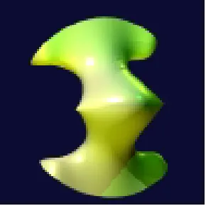
1.2 The Steiner surfaceS . . . 3
1.3 q(s,t) := s2+t2+s−t+1=0 does not have any real solutions. . . . 3
1.4 The image of the mapris contained in the surfaceS . . . 4
1.5 The intersection of the image of the parametrizationrwith planey= 1. . . 4
1.6 The intersection of Steiner surfaceS with planey=1. . . 5
1.7 The intersection of Steiner surfaceS with planey=1. . . 6
1.8 The points on Steiner surfaceS and the planey=1 which do not belong to the intersection of the image of the parametrizationrgiven by (1.2) and the plane y=1. . . 7
1.9 Closure of Image(r). . . 7
1.10 The tangent cone of the fish given by f := y2− x2(x+4)= 0 at the origin . . . 8
1.11 Intersection multiplicity . . . 9
1.12 The surface defined byq=zaround the origin. . . 10
1.13 A surface and the paths represented by its discriminant variety . . . 12
1.14 Separating the branches of the curve given by f :=y(x−2)2+x= 0 . . . 13
1.15 RegularChainBranchescommand for regular chainrc . . . 13
2.1 The eve surface . . . 20
2.2 The real solutions ofV(F) computed byRealTriangularize . . . 20
2.3 The complex solutions ofV(F) computed byTriangularize . . . 21
2.4 Weierstrass Preparation Factorization and Extended Hensel construction . . . . 22
2.5 Extended Hensel construction applied to a bivariate polynomial . . . 22
3.1 EHC applied to a trivariate polynomial. . . 26
3.2 Computational of limit points: complex and real cases. . . 28
3.3 Comparison of three different implementations of EHC algorithm . . . 42
5.1 Computing the limit points of a regular chain: complex case vs real case. . . 67
7.1 The planner curve called ”fish” and its tangent cone at the origin . . . 102
7.2 Limiting secants alongV(x2+y2+z2−1, x2−y2−z). . . 111
7.3 Secants alongV(x2+y2+z2−1)∩V(x2−y2−z(z−1)) limiting to (0, 0, 1). . 113
8.1 The graph corresponding to g(xf(x,,y)y) =z . . . 133
8.2 Limit of real bivariate rational functions . . . 134
List of Tables
3.1 The total number of multiplications and additions ofM1M2 . . . 39
3.2 Comparing EHC versus Kung-Traub’s method (timings are in seconds) . . . 43
4.1 Removing redundant components. . . 64
5.1 Complex limit points vs real limit points . . . 75
8.1 Comparisons of the commandslimit,TestLimit, andRationalFunctionLimit . . . 136
Chapter 1
Overview
In computational mathematics, computer algebra, also known as symbolic computation, is an area that develops algorithms and software for solving mathematical problems by means of exact computation. Here, exact computation implies that mathematical entities are represented by their formal definitions instead of using approximations. For instance, computer algebra algorithms may represent √2 as the positive solution of x2 = 2 while numerical methods would generally use a floating point approximation like 1.414213562.
The software that perform symbolic computations are called computer algebra systems. Some of the most famous computer algebra systems includeSingular,Aldor, Maple,Mathematica, AXIOM, CoCoA, MAGMA, and many others. Development of computer algebra systems began in 1960s mainly to serve the two fields of theoretical physics and Artificial Intelligence1.
Nowadays, general-purpose computer algebra systems can solve a wide range of mathe-matical problems from factoring an integer number, solving linear systems, determining the real roots of a univariate polynomial to solving a system of non-linear equations, and solving a system of partial differential equations (see Figure 1.1). Hence, computer algebra systems ma-nipulate numbers, matrices, polynomials and other algebraic objects. These capabilities stems from the fact that many algebraic properties can be stated in terms of closed-form expressions and established by means of rewriting systems.
While computer algebra systems can perform highly sophisticated algebraic tasks, such as solving (formally) a system of partial differential equations, they are much less equipped for solving problems from analysis in a symbolic, or exact manner. Some problems in analysis, like the manipulation of Taylor series and the calculation of limits of univariate functions, that is essentially undergraduate univariate calculus, is available (with some limitation) in general-purpose computer algebra systems such as MapleandMathematica. However, limits of
mul-tivariate functions and more advanced notions of limits, e.g. topological closures, are almost absent from such systems. For instance, Mapleis not capable of computing limits of rational
functions in more than two variables.
Many fundamental concepts in mathematics are defined in terms of limits and it is desir-able for computer algebra to implement those concepts. However, they are, by essence, hard to compute, or even not computable, in an algorithmic fashion, say by doing finitely many
1Seehttps://en.wikipedia.org/wiki/Computer_algebra_system for more details about computer
algebra systems, as of May 2017.
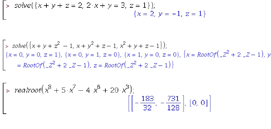
Figure 1.1: The computer algebra system Maple uses commands solve and RealRoot to
solve polynomial systems; the commandsolvecan solve both linear and non-linear systems; the commandRealRootisolates the real roots of univariate polynomials in intervals.
rational operations on polynomials or matrices, over the usual coefficient fields of symbolic computation.
Let us give an example of a limit computation process by means of computer algebra tools. This example is taken from Computer Aided Geometric Design and uses an important question raised in studying algebraic surfaces. Given an algebraic surfaceS ⊆R3and a parametrization
of S described by the following mapping:
r: R2 → R3
(s,t) 7→ r(s,t)
determine whether Image(r)= S holds or not. That is, determine whether every point ofS can be reached with the parametrizationr.
Consider the Roman surface or Steiner surface2(see Figure 1.2) with implicit formula f = 0, where f is the following polynomials in the variablesx,y,z:
f :=4x4−8yx3+9x2y2−8yzx2−5y3x+8y2zx+y4
−2y3z+3y2z2−2yz3+z4−8yx2+8zx2+8y2x
−8xyz−2y3+2y2z−2yz2+4x2−4yx+y2.
(1.1)
Withq(s,t) := s2+t2+s−t+1, consider also the following map
r: R2 → R3
(s,t) 7→ q(ss2,t) , q(ss2+,tt)2 , s2+q(ss t+,t)s+t, (1.2) 2seehttps://en.wikipedia.org/wiki/Roman_surfacefor more information about Steiner, also called
3
Figure 1.2: The Steiner surfaceS (this image is taken from [86]).
We want to determine whether Image(r) = S holds or not. TheMaple session shown on Figure 1.3 proves thatq(s,t) does not vanish over the reals while theMaplesession shown on Figure 1.4 implies that Image(r)⊆ S holds.
Figure 1.3: q(s,t) := s2+t2+ s−t+1=0 does not have any real solutions.
We now verify that the equality Image(r) = S does not hold. To do so, we shall compare the points of Image(r) satisfyingy= 1 with the points ofS satisfyingy= 1.
First, we compute the intersection of the image of the parametrization r with the plane y = 1. This can be determined to be the ellipse calculated in the Maple session shown on Figure 1.5, namely the plane curve with Cartesian equation:
2x2+2x z+z2−3x−2z+1=0.
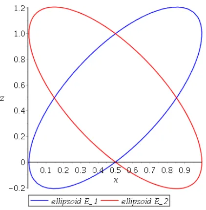
Next, if we substitutey=1 in the implicit formula f =0 of Steiner surface (see Figure 1.6), then we obtain
(2x2−2x z+z2− x) (2x2+2x z+z2−3x−2z+1)= 0
yielding two different ellipsesE1andE2, see Figure (1.7).
Thus the parametrization r does not cover the ellipse E1 related to the first factor, see
Figure 1.8. In fact, more advanced calculations can show that the points that are missed by the parametrizationrare exactly those points belonging to E1and not toE2.
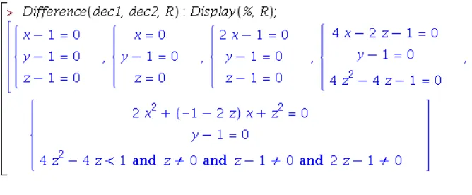
Figure 1.4: The command Difference computes the points in the image of r that do not belong to surfaceS, which is empty.
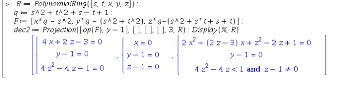
Figure 1.5: The intersection of the image of the parametrization rwith planey=1.
systemRshown in Equation (1.3)
R:=
q(s,t)x−s2 =0 q(s,t)y−(s2+t2)= 0
q(s,t)z−(s2+s t+s+t)= 0
q(s,t), 0
(1.3)
Broadly speaking, Theorem 2 in [29] implies that eliminating s,tfrom the polynomial system Ryields a polynomialgsuch that the topological closure of Image(r) is exactly the zero set of g. TheMaplesession of Figure 1.9 shows that this polynomialgis precisely the polynomial f introduced in Equation (1.1).
Therefore, our original question, that is, checking whether Image(r) ⊆ S holds or not, can be answered by
5
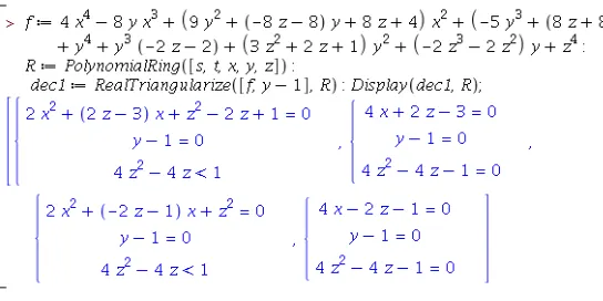
Figure 1.6: The intersection of Steiner surfaceS with planey=1.
Note that comparing the topological closure of Image(r) against Image(r) will produce the points missed by the parametrizationr.
Computing topological closures of solution sets of polynomial systems, and thus computing missing points of parametrizations, are the questions motivating this thesis.
To see how those latter questions can be addressed in terms of limit computations, we intro-duce some notations before considering two examples. LetW be the zero set of a polynomial system R and let W be the topological closure of W in the Euclidean topology. Often W is known whileW is to be computed. In the previous example, the setW was Image(r). In the next, and simpler example, we shall see that the set-theoretic differenceW\Wcan be obtained via a limit computation process. Consider the following systemR
R:=
z x−y2 =0
y5−z4 =0 z,0
. (1.4)
Let us denote byW the set of all (x,y,z)∈C3 solvingR. A natural parametrization3ofW can be given by
(
x= yz2 y=z4/5 ,
whereznow can play the role of a parameter. To be more formal, we can write this parametriza-tion as
x= t8t/5 y= t4/5 z= t
,
wheretis a parameter. For this parametrization,z(and consequentlyt) can accept any complex value but zero in order to be able to determine the values ofxandy.
To computeW\W, that is, the possible missing points of that parametrization, we compute the limit ofx,y,z, regarded as functions oft, att=0. Thus we have:
Figure 1.7: The intersection of Steiner surfaceS with planey=1.
limt→0z=limt→0t=0,
limt→0y=limt→0t4/5 =0,
limt→0x=limt→0 y2
t =limt→0 (t4/5)2
t =limt→0t
3 5 =0.
Therefore, (0,0,0) is a missing point, or in other words, a limit point of the set W in the Euclidean topology.
Let us consider now this other system, which is a variation of (1.4) in which the termz4in the second equation is replaced withz2:
z x−y2 =0
y5−z2= 0
z,0
. (1.5)
The following is a parametrization of the above system:
x= t4t/5 y= t2/5 z= t
.
Therefore,
limt→0z=limt→0t= 0,
limt→0y=limx1→0t
2/5 =0,
limt→0x=limt→0 y2
t =limt→0 (t2/5)2
t = limt→0 1
t15 =
±∞.
7
Figure 1.8: The points on Steiner surface S and the planey = 1 which do not belong to the intersection of the image of the parametrizationrgiven by (1.2) and the planey= 1.
Figure 1.9: Closure of Image(r).
The above approach, which is based on computing the limits of different variables, is an inspiring method. However, there is a difficulty in applying this approach to more advanced cases. To see this, let us have a look at a slightly more complicated example and consider the solution setWof the systemRin the variablest,y,x, given by:
R:=
(t+2)t x2+(y+1) (x+1)= 0 t y5−y+1=0
(t+2)t,0
, (1.6)
where the variablet is regarded as a parameter. In order to apply the same process as before, one needs to computexandyas functions int. For the last two examples, this was really easy. But now the obstacle is how to find such functions in general.
• the computation of the tangent cone of a space curve at one of its singular points, and
• the computation of limits of multivariate rational functions.
In the rest of this chapter, the main goals of this thesis are presented followed by our accomplishments towards those goals. We end this chapter by giving a brief overview of all chapters presented in this thesis.
1.1
Goals
In this thesis, we have three main objectives that we explain in this section.
Our first and most important goal is to compute the topological closures, or equivalently limit points, of solution sets of polynomial systems. The examples that we used above suggest to use parametric representations of such sets. To be technically more precise, they suggest to use representations given by rational functions. Unfortunately, this is not always possible and one needs to use a weaker notion of “parametrization”, which is given by that of aregular chain4.
Using the fact that the solution set of every polynomial system (over the complex number as well as over the reals) can be decomposed into the solution sets of finitely many regular chains, we restate our main objective as follows, where all technical terms are defined in Chapter 2.
Given a regular chainR⊂Q[x1, . . . ,xn], denoting byhRthe product of its initials, our goal
is to compute the (non-trivial)limit pointsof both
1. the setZR(R) consisting of the real zeros ofRwhich do not cancelhR, and
2. the setW(R) consisting of the complex zeros ofRwhich do not cancelhR.
In other words, denoting by ZR(R) and W(R) the closures of ZR(R) and W(R) in the Eu-clidean topology and Zariski topology, respectively, we want to determine the set lim(ZR(R)) :=
ZR(R)\ZR(R) and lim(W(R)) :=W(R)\W(R).
Figure 1.10: The tangent cone of the “fish” given by f := y2 − x2(x+ 4) = 0 at the origin
consists of two tangent lines: y=2xandy=−2x.
Our second objective is to compute the tangent cone5of a space curve at one of its singular
4The notion of regular chain will be defined formally in Chapter 2.
5The tangent cone of a space curve at one of its points is a linear approximation of that curve around that point,
1.2. Thesis accomplishments 9
> F :=h(x2+y2)2+3x2y−y3,(x2+y2)3−4x2y2i:
>plots[implicitplot](F s,x=−2..2,y=−2..2) :
>R:= PolynomialRing ([x,y],101) : >TriangularizeWithMultiplicity(F,R);
""
1,
(
x−1=0 y+14=0
## ,
""
1,
(
x+1=0 y+14=0
## ,
""
1,
(
x−47=0 y−14=0
## , ""
1,
(
x+47=0 y−14=0
## ,
""
14,
( x=0 y=0
##
Figure 1.11: In the RegularChains library in Maple, the command TriangularizeWithMul-tiplicity computes the intersection multiplicity of V(F) for all the points p ∈ V(F). In the above Maple session, computations are performed modulo a prime number for the only rea-son of keeping output expressions small. The same calculations can be performed with the TriangularizeWithMultiplicitycommand over the reals.
points without relying on standard basis computations. This topic is a follow-up on a prelimi-nary work by S. Marcus, M. Moreno Maza and P. Vrbik on computing intersection multiplic-ities of zero-dimensional algebraic sets by means of regular chain theory [62]. Figure 1.11 illustrates how the RegularChains library in Maple computes triangular decomposition of zero-dimensional algebraic sets together with intersection multiplicities. In [62], the authors reduce their problem to that of computing the tangent cone of a space curve at one of its singu-lar points. Therefore, the second objective of this thesis aims at completing the project initiated in [62].
Our third and final objective deals with the computations of limits of real multivariate ra-tional functions. For example, for the multivariate rara-tional functionq = x4+3xx22+y−y2x2−y2, we are interested in determining whether lim(x,y)→(0,0)qexists or not, and, if it exists, to compute it, see
Figure 1.12.
1.2
Thesis accomplishments
Figure 1.12: The surface defined byq= zaround the origin.
1.2.1
Computing limit points of quasi-components of regular chains of
dimension one.
Regarding the first objective, that is, computing the limit points of solution sets of polynomial systems, we have established a method for computing limit points of solution sets of regular chains in dimension one, see Chapter 4 and the article [6] co-authored with C. Chen and M. Moreno Maza. Puiseux expansions play a central role in our results. The work presented in Chapter 4 focuses on limit points corresponding to the regular chains of dimension one with respect to Zariski topology.
1.2.2
Improving the extended Hensel construction.
For computing Puiseux series expansions, we were initially relying on thepuiseuxcommand of thealgcurve package of Maple. This command only accepts input polynomials with two
variables and, consequently, cannot be used for computing Puiseux parametrizations of regu-lar chains with dimension higher than one. Therefore, a complete implementation computing Puiseux expansions of algebraic functions in several variables was needed. Up to our knowl-edge, there is only one practical method meeting our needs, namely the so-called extended Hensel construction (EHC, for short) a method introduced by T. Sasaki and F. Kako in [82]. Our current implementation of the EHC is integrated into thePowerSeries6package of Maple.
In Chapter 3, a short review of the EHC is followed by our new techniques for improving the computational efficiency of that algorithm. We show that the EHC requires only linear alge-bra and univariate polynomial arithmetic. We deduce complexity estimates and report on a software implementation together with experimental results. This is a joint work with Masoud Ataei and Marc Moreno Maza.
1.2. Thesis accomplishments 11
1.2.3
Computing the real limit points of the quasi-component of a regular
chain of dimension one.
One of the interesting facts about the EHC is the following. Suppose that, for a bivariate polynomial F ∈ K[X,Y], where K is a field extension of Q (the field of rational numbers) we want to factor F into linear factors in X over the field of Puiseux series of Y. Then, the EHC will not only determine the algebraic extension L of K necessary to do so, but it will also, for each linear factor ofF, characterize the sub-field ofLwhich is required to express the coefficients of that factor. Thanks to this fact, we have proposed a method for computing the ”real” limit points of regular chains of dimension one in Chapter 5; see also Section 5 in [3].
1.2.4
Studying regular chains under changes of coordinates.
As mentioned above, the ideas presented in Chapters 4 and 5 (respectively for computing the complex and real limit points of the quasi-components of regular chains) are only applicable to regular chains with dimension one. Therefore, a complete algorithm is still needed to compute the limit points of quasi-components of regular chains in higher dimension. That is why we take the second approach presented in Chapter 6 and [4]. Broadly speaking, the intention is to map the limit point computation from a coordinate system where it is difficult to perform to another coordinate system where it is easy to do. We do not propose a general method achieving this intention, but we propose criteria which appear to be helpful in practice.
1.2.5
Introducing new tools for computing tangent cones of space curves.
Computing limit points of quasi-components of regular chains can be applied to perform other ”limit computations”. The first example, discussed in Chapter 7, is the computation of the tangent cone of a space curveC(and more generally algebraic set) at one of its points, say P. Indeed, the tangent cone ofCatPis the set of the limits of the secantsPQwhereQis a point on
CapproachingP. Taking advantage of this method, in Chapter 7, we have proposed a method for computing the tangent cone of algebraic curves, which is the main tool for computing the intersection multiplicity of algebraic curves at any point. This means we have also met our second objective of this proposal for computing the tangent cones of space curves at their singular points.
1.2.6
Computing limit of real multivariate rational functions.
Regarding the last objective of this dissertation, we have answered the questions of
1. how to determine whether the limit of a real multivariate rational function at the origin exists or not, and
2. if it exists, how to compute it,
respectively computing the limit of real bivariate and trivariate rational functions at the origin when the origin is an isolated zero of the denominator. The key point in this method is that for computing the limit of a multivariate rational functionqat the origin, it is enough to compute the limit of q at the origin along a finite number of special paths, represented by a so-called discriminant variety. For example, for the real multivariate rational functionq:= x4+3xx22+yy−2x2−y2, see Figure 1.13, its discriminant variety consists of three different paths through the origin. Following each of them, one can verify that the limit ofqat the origin exists and is equal to
−1.
For covering the case when the origin is not an isolated solution of the denominator, we suggest possible directions, in particular by following the paper [54] in which the L’Hospital’s rule for multivariate rational functions is introduced. It is worth noting that in 2014, S.J. Xiao and G.X. Zeng, in [104], proposed a first algorithm that decides whether lim(x1,...,xn)→(0,...,0)qis zero or not, without any assumptions on the denominator of q. However, the results of our experimentation shows that our implementation outperforms the one in [104].
Figure 1.13: On the left: the surface defined byq:= x4+3xx22+y−y2x2−y2 = zaround the origin. On the right: the three paths of discriminant variety ofqgoing through the point (0,0,-1).
1.2.7
Separating the real and complex branches of space curves.
For computing the limit of a real multivariate rational function q at the origin, one needs to compute local parametrizations of all the paths represented by the discriminant variety (in the sense of the papers [21] and [98]) ofqaround the origin. In the set up of the method described in Chapter 8 and also [8], we represent the discriminant variety of q as the union of finitely manyregular semi-algebraic sets. Thus for computing and separating all of those special real paths, we compute real Puiseux parametrizations corresponding to all of the regular chain parts of the regular semi-algebraic sets representing the discriminant variety of qat the origin, see Figure1.13. In fact, we propose a method for separating the real and complex branches of space curves given by regular chains from the ones that escape to infinity when the parameter corresponding to the given curve approaches zero, see Figure 1.14.
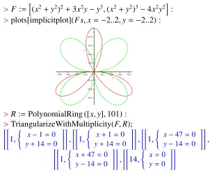
1.2. Thesis accomplishments 13
Figure 1.14: On the right: Close to the origin, the irreducible polynomial f := y(x−2)2+ x
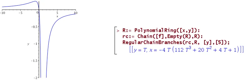
contains two different paths: one passing through the origin and the other one not. On the left: RegularChainBranches returns a parametrization for the path of f going through the origin.
chain might have more branches than the ones printed in the output ofRegularChainBranches. In fact, those branches corresponding to the given regular chain that escape to infinity, when the parameter of the given regular chain approaches zero, are excluded from the output of the commandRegularChainBranches(see Figure 1.15).
Figure 1.15: The commandRegularChainBranchescomputes a parametrization for the com-plex and real paths of the quasi-component defined byrc. When coefficient argument is set as real, then the commandRegularChainBranchescomputes the real branches.
1.2.8
Thesis contribution in
RegularChains
and
PowerSeries
libraries.
The recent progress on regular chain theory and all the new features added toRegularChains
input multivariate polynomial with respect to its main variable, is integrated intoPowerSeries
library. The source code of both theRegularChainsandPowerSerieslibraries are available athttp://www.regularchains.org/.
1.3
Contribution statement
Each chapter of the present thesis, except Chapter 2, is based on a refereed publication. In the sequel, we discuss the relations between those publications and chapters, as well as co-authors’ contributions.
The work presented in Chapter 3, about the extended Hensel construction, is accepted at the ISSAC 2017 conference [3]. This is a joint work with Marc Moreno Maza and Masoud Ataei.
The method presented in Chapter 4, for computing complex limit points of regular chains of dimension one with respect to Zariski topology, is a joint work with Marc Moreno Maza and Changbo Chen. It was published in 2013 in the CASC conference [6].
The method for finding the real limit points corresponding to the regular chains of dimen-sion one, which forms Chapter 5, is mainly the work of the author of the present thesis; it is also presented in Section 5 of [3].
The materials presented in Chapter 6, except Section 6.3.1, were published in 2015 in the CASC conference [4]; this is a joint work with Marc Moreno Maza, Amir Hashemi, and Changbo Chen. Section 6.3.1 in Chapter 6 is about thePALGIE algorithm, which was orig-inally introduced in [18, 20] by Franc¸ois Boulier, Franc¸ois Lemaire and Marc Moreno Maza for differential regular chains. We present this algorithm in a purely algebraic setting and ex-tensions of his specifications are proposed; this work was done by Marc Moreno Maza and the author of the present thesis.
The work presented in Chapter 7, based on the CASC 2015 article [9] by the author of the present thesis with Marc Moreno Maza, ´Eric Schost, and Paul Vrbik. In fact, this work builds upon the PhD thesis of Paul Vrbik, see [100] and is an application of computing limit of quasi-components of regular chains.
Finally, the materials forming Chapter 8 are mainly taken from the ISSAC 2016 article [8]. This is a joint work of the author of the present paper with Marc Moreno Maza and Mahsa Kazemi.
1.4
Thesis outline
This thesis contains seven different chapters, in addition to the current one.
Chapter 2 provides definitions and notations used throughout this thesis about our main tools, namely regular chains and Puiseux series expansions. It also provides some information about the related work.
1.4. Thesis outline 15
initial factors of the Newton polynomial. To do so, we suggest an efficient algorithm together with complexity estimates in Section 3.3. The second step is to compute the product of the lifted factors at each iteration. In Section 3.4, we explain our method for multiplying the lifted factors, efficiently; in particular, we demonstrate how to recycle the computations performed in previous iterations. Finally, in Section 8.7, we present experimental results comparing our improved EHC against the original one.
In Chapter 4, we address the problem of computing (non-trivial) limit points induced by regular chains of dimension one with respect to Zariski topology. The method described in Chapter 4 for computing such limits is via Puiseux series expansions. We first establish the no-tion of Puiseux parametrizano-tions for regular chains of dimension one around a point vanishing the product of the initials of the polynomials contained in the given regular chain. By using a few of the first terms of such Puiseux series appearing in the Puiseux parametrizations of a regular chain, one can compute the desired limit points. Later on, we give several results on how to truncate the series appearing in the Puiseux parametrizations while having sufficiently many terms to calculate the limit points. We conclude Chapter 4 by an application of finding limit points corresponding to regular chains in removing redundant components in triangular decompositions of polynomial systems.
In Chapter 6, we discuss how to compute limit points of quasi-components of regular chains via changes of coordinates. The results in this chapter cover the case where regular chains have positive dimension and not necessarily dimension one. One of the main challenges in this method is that after applying a change of coordinates to a regular chain, the resulted polyno-mial set might not be a regular chain. Our goal is, then, to replace this polynopolyno-mial set by one regular chain at a “cheap computational cost. We achieve this by employing the PALGIE algo-rithm [18, 20] We also consider Noether normalization and its effect on regular chains structure. Finally, we present several results for computing the limit points of quasi-components of the regular chains with respect to Zariski topology.
Chapter 7 describes our method for computing the tangent cones of a space curve at one of its singular points. As explained in Section 1.1, the main idea is to compute limits of families of secant lines; this trick permits a reduction to the computations of limit points of quasi-components of regular chains in dimension one.
In Chapter 8, we discuss how to compute the limit of real multivariate rational functions at the origin. We first present our method for computing such limits when this latter point is an isolated zero of the denominator. This work was published in [8]. Section 8.3 states fundamental lemmas as the main ingredients to the proof of the correctness of Algorithm 20, in Section 8.4. Then, in Section 8.6, we suggest how to compute the limits of real multivariate rational functions at the origin when this latter point is not an isolated zero of the denominator. Finally, Chapter 9 summarizes the accomplishments of the present thesis for addressing the main goals of this thesis. Chapter 9 also discusses the problems that have remained unsolved with respect to our goals.
All the algorithms presented in this thesis are implemented in Mapleand are integrated into
Chapter 2
Background and Related Work
In this chapter, we gather definitions and notations used throughout this thesis. The problem of computing limit points of regular chains is also explained more formally. Moreover, related works are also discussed.
2.1
Solving polynomial systems
Solving linear polynomial systems is a cornerstone in mathematical sciences. This problem has been at the centre of attention of many researchers in both the academia and the industry, yielding fast algorithms and efficient implementation. However, replacing linear systems with nonlinear ones results in a dramatic decline in what can be achieved in practice, due to the inherent higher complexity of the problem. This is especially true when exactness and com-pleteness are required features for the computed solution sets. Therefore, it is desirable for symbolic methods, which aim at providing these features, to emphasize the development of better and better algorithms for solving polynomial systems.
Among all the avenues by which such systems can be solved, the one significant method is triangular decomposition, see [19, 25, 22, 11], which decomposes each nonlinear system into several components, with special shapes and rich properties, calledregular chains.
Before stating formal definitions, we start with an example. Consider the polynomial set F := {f1, f2, f3}where the polynomials
f1 = x2+y+z−10, f2 =y2+x+z−1, f3 =z2+x+y−1
have rational number coefficients and three variables z,y,x, that we order as z < y < x. The solution set ofF, that is, the set of the points (x,y,z) with complex coordinates satisfying
f1 = f2= f3 =0,
can be decomposed as follows into four components:
R1 :=
x−z= 0 y−z= 0 z2+2z−1= 0
, R2 :=
x=0 y=0 z−1=0
, R3 :=
x= 0 y−1=0 z= 0
, R4:=
x−1= 0 y=0 z=0
.
2.1. Solving polynomial systems 17
Each of the polynomial sets defining those components has a triangular shape and is called a regular chains. In our example, we denote these four regular chains by R1,R2,R3,R4
respec-tively and we say that{R1,R2,R3,R4}forms a triangular decomposition forF. As one can see,
it is easy to read the solutions for each of the regular chainsR1,R2,R3,R4, even if, forR1, a bit
of work is needed (solving the equation inzand substituting in the other two equations). Let X1, . . . ,Xn be n independent variables. A monomial in variables X1, . . . ,Xn is of the
formXα1
1 · · ·X
αn
n , whereαi ∈Z≥0, fori= 1, . . . ,n. For convenience, we denote a monomial as
Xα. The degree of this monomial is defined asα1+· · ·+αnand denoted by deg(Xα).
The set all of the polynomials in X1, . . . ,Xn with coefficients in the field kis denoted as k[X1, . . . ,Xn], ork[X], and is called apolynomial ring over k. In this thesis, we are mainly
interested in polynomial rings over the real and complex numbers, that is, whenkis the field of real or complex numbers.
Let X1 < · · · < Xn be an order on these variables. For a non-constant polynomial f, the
greatest variable appearing in f is called themain variableof f, denoted by mvar(f), and the leading coefficient of f w.r.t. mvar(f) is called the initial of f, denoted by init(f). These notations support algorithms where the polynomial f is considered as a univariate polynomial in its main variable.
Example 1. For f =2X1X22+X2 ∈Q[X1,X2], its main variable is X2and its initial is2X1.
Letkbe a field andkbe its algebraic closure1. Since in this thesis, the fieldkwill often be the fieldRof the real numbers or the field Cof the complex numbers, we havek = C. For a
polynomial setF ⊆k[X], the set of all common solutions (or zeros) of the polynomials in Fis denoted byV(F) and called thealgebraic set, oralgebraic variety, ofF. Hence, we have:
V(F) := {(a1, . . . ,an)∈k n
| f(a1, . . . ,an)=0 for each f ∈F},
.
Example 2. Let F ={X1+X22,X21+X2} ⊂C[X1,X2]. Then
V(F)=
(0,0),(−1,−1),(1+i
√
3 2 ,
1−i√3 2 ),(
1−i√3 2 ,
1+i√3 2 )
.
It is worth mentioning that the solutions of a polynomial system depend on the field over which the solutions are searched for. For instance, in Example 2, if we solveFoverQthen we
have
VQ(F)={(0,0),(−1,−1)}.
Definition 1. A set R of non-constant polynomials ink[X]is said to be atriangular set, if for
all f,g ∈R, with f , g, we havemvar(f), mvar(g).A variable Xi is saidfreew.r.t. R if there
is no f ∈R such thatmvar(f)= Xi, otherwise, it is saidalgebraic.
Example 3. Consider the set R defined as following:
R=
(
r2 :=X1X3−X22
r1 :=X24−X15
⊆Q[X1,X2,X3].
Then, R is a triangular set sincemvar(r2)= X3, mvar(r1)= X2. Moreover, X1is the only free
variable of this set.
Definition 2. A setI ⊂k[X1, . . . ,Xn]is an ideal if it satisfies the following conditions:
1. 0∈ I,
2. if f,g∈ I, then f +g∈ I, and
3. if f ∈ Iand h ∈k[X1, . . . ,Xn], then h f ∈ I.
Lemma 1 (See [29], Chapter 1, Lemma 3). Let f1, . . . , fs be polynomials in k[X1, . . . ,Xn].
Consider the set defined as follows:
hf1, . . . , fsi:=
s X
i=1
hifi |h1, . . . ,hs ∈k[X1, . . . ,Xn]
.
Then, the sethf1, . . . , fsiis an ideal and is called the ideal generated by f1, . . . , fs.
Definition 3. For a nonempty triangular set R, we define the saturated ideal of R, which is
denoted bysat(R), to be the ideal
hRi:h∞R :=
f ∈k[X]| ∃m∈N:hmRf ∈ hRi ,
where hR is the product of the initials of the polynomials in R. The saturated ideal of the empty
triangular set is defined as the trivial ideal.
The ideal sat(R) has several properties, in particular it is unmixed (see [19]). We denote the number of polynomials inRbye. It turns out that sat(R) has dimensionn−e(see Theorem 1.6 in [19]). Moreover, writingR= {r1, . . . ,re}and assuming mvar(ri)= Xn−e+i, for 1≤ i ≤ e, the
intersectionk[X1, . . . ,Xn−e]∩sat(R) is the trivial idealh0i.
Definition 4. Let I ⊂ k[X1, . . . ,Xn] be an ideal. A polynomial is regular modulo I, if it is
neither zero nor a zero-divisor2moduloI.
Definition 5. We say that the triangular set R = {r1, . . . ,re}is a regular chain whenever R is
empty or {r1, . . . ,re−1} is a regular chain and the initial of re is regular modulo the saturated
ideal sat({r1, . . . ,re−1}). The regular chain R is said to be strongly normalizedwhenever no
algebraic variables appear in the initials of the polynomials of R,
Example 4. One more time consider the triangular set
R:=
(
X1X3−X22
X4 2 −X
5 1
.
Then R is a regular chain because hR = X1 is regular modulosat({r1}) = hX24− X15i, where
r1 := X24−X15. Indeed, the regularity of a polynomial modulo the saturated ideal of a regular
chain can be checked using pseudo division (see [25]).
2.1. Solving polynomial systems 19
Definition 6. We denote by W(R) := V(R) \ V(hR) the quasi-component of R, that is, the
common zeros of R that do not cancel hR.
Definition 7. Let S ⊂ kn. The Zariski closure of the set S , denoted as S , is defined to be
V(I(S))where
I(S)={f ∈k[X1, . . . ,Xn]| f(a)= 0for all a∈S}.
It can be proved that S is also the intersection of all algebraic sets containing S , that is, the smallest algebraic set containing S .
Regular chains enjoy many properties. In particular, the quasi-component W(R) of the regular chain is not empty. Moreover, the Zariski closure of W(R) satisfies the following: W(R)= V(sat(R)).
Definition 8. Let F ⊂ k[X]. The regular chains R1, . . . ,Rs of k[X] form a triangular
de-composition of V(F) in the sense of Kalkbrener (resp. Wu and Lazard) whenever we have V(F) = ∪s
i=1W(Ri)(resp. V(F) = ∪ s
i=1W(Ri)). We denote byTriangularizean algorithm, such
as the one in [25], computing a Kalkbrener triangular decomposition.
Regular chains are defined in multivariate polynomial rings where coefficients are them-selves in a (commutative) ring. In practice, coefficients are often rational numbers while the values of the unknowns are either complex or real numbers. In the latter scenario, it is desirable to have an algorithm decomposing the solutions of polynomial systems overRrather than over C. This is done by another algorithm calledRealTriangularizeintroduced in [22] by C. Chen,
J. H. Davenport, J. P. May, M. Moreno Maza, B. Xia and R. Xiao.
Example 5. Let F := {5y6 −15y5 + 15y4 + 2x z2 − 5y3 + 5x2 + 5z2} ⊂
Q[z < y < x].
The command RealTriangularize in the RegularChains library inMaple can solve for
the real solutions of F, see Figure 2.2. These real solutions form the so-called Evesurface displayed on Figure 2.13. On the other hand, the command Triangularize can solve the
complex solutions of the above system as illustrated on Figure 2.3.
Regular chains can be used to represent the solution sets of systems of equations, inequa-tions and inequalities. More generally, they support the implementation of set-theoretic oper-ations (union, intersection, difference) of algebraic sets, constructible sets, and semi-algebraic sets. To illustrate the difference between triangular decompositions in the sense of Kalkbrener, and triangular decompositions in the sense of Lazard and Wu (see Definition 8) we consider the following example.
Example 6. For the variable order b < a < y < x, consider the polynomial set F = {a x+
b,b x+y}and the regular chain R1= {b x+y,a y−b2}. Using calculations inMaple, one can
verify that we have
V(F)= W(R), (2.1)
3This image is taken from the gallery of algebraic surfaces athttp://homepage.univie.ac.at/herwig.
Figure 2.1: The eve surface
Figure 2.2: The real solutions ofV(F) computed byRealTriangularize
which means that{R1}is a triangular decomposition of F in the sense of Kalkbrener. Using the
notion oflocalizationin algebra 4, it is possible to interpret Equation (2.1) by stating that R1
describes the solutions of F of the following form:
(
x= −y
b
y= ba2 ,
for any complex value of a and b where a b , 0. However, this latter solution set is missing the solutions of F given by the regular chains R2 ={x,y,b}and R3 = {y,a,b}. In fact, one can
easily verify, withMaplecalculations, that the following holds:
V(F)=(V(R1)\V(a b)) ∪ V(R2) ∪ V(R3),
which means that {R1,R2,R3}is a triangular decomposition of F in the sense of Lazard and
Wu.
In Example 8, one can see that we have
W(R1)\W(R1) = V(R2) ∪ V(R3),
that is, the limit points ofW(R1) in Zariski topology consist ofW(R1) and the two lines given
byV(R2) andV(R3). At this point, we review the notion of a limit point.
2.2. Power series andPuiseux expansions 21
Figure 2.3: The complex solutions ofV(F) computed byTriangularize
2.1.1
Limit points
Let (X, τ) be a topological space. A point p ∈ X is alimitof a sequence (xn,n ∈ N) of points
of X if, for every neighbourhood U of p, there exists an N such that, for every n ≥ N, we have xn ∈ U; when this holds we write limn→∞ xn = p. If X is a Hausdorffspace then limits
of sequences are unique, when they exist. Let S ⊆ X be a subset. A point p ∈ X is alimit pointofS if every neighbourhood of pcontains at least one point ofS different from pitself. Equivalently, p is a limit point ofS if it is in the closure ofS \ {p}. In addition, the closure of S is equal to the union of S and the set of its limit points. If the space X is sequential, and in particular if X is a metric space, the point p is a limit point of S if and only if there exists a sequence (xn,n∈N) of points ofS \ {p}with pas limit. In practice, the “interesting”
limit points ofS are those which do not belong toS. For this reason, we call such limit points non-trivialand we denote by lim(S) the set of non-trivial limit points ofS.
Definition 9. For the regular chain R ⊂ k[X1, . . . ,Xn] a point p ∈ k
n
is called a limit point of R, if it is a limit point of W(R) in the above topological sense. Further, the point p is said anon-triviallimit point of R if it is a non-trivial limit point of W(R). The set of all non-trivial limit points of W(R)is denoted bylim(W(R)). From now on, when we talk about the limit points of a quasi-component of a regular chain, we actually refer to its non-trivial limit points.
2.2
Power series and Puiseux expansions
In mathematics, Puiseux series are a generalization of power series. As we know, power series are used to approximate an analytic function with a polynomial about a point. As an example,
1 1−x =
P∞
i=0x
i = 1+x+ x2+ x3+· · · is the power series expansion of the function 1
1−x about
x = 0. Now one might ask the question of how to approximate a plane algebraic curve about one of its points, in particular singular points. In this case, such curve may not be seen as the graph of an analytic function, even locally. Puiseux series address this more general setting. A Puiseux series5in xtypically looks like
∞
X
i=k
cix
i d,
wheredis a positive integer andkis an integer, possibly negative.
(Univariate) Puiseux series inX1, with complex number coefficients, form an algebraically
closed field, denoted byC((X∗
1)). Consequently, any bivariate polynomialF ∈C[X1,X2] can be
factored into linear factors inX2 with coefficients inC((X1∗)). This result, known as Puiseux’s
theorem, has a geometrical interpretation. These linear factors correspond to the branchesof the plane curve6 F(X
1,X2) = 0 around the origin. Being able to compute the branches of a
plane curve around one of its points will be an essential tool in Chapter 4, upon which we will build our algorithm for computing the limit points of regular chains with one free variable.
Example 7. By factoring the polynomial F := X1X23+X22+X2+X1, overC((X∗1)), we obtain
the following three linear factors:
• X2+1,
• X2+X1+X12+O(X31),
• X2+ X11 −1−X1−X
2
1 +O(X 3 1),
and thus a description of the branches of F(X1,X2)= 0around the origin:
• X2 =−1,
• X2 =−X1−X21+O(X13),
• X2 =−X11 +1+X1+X
2 1+O(X
3 1),
Since Puiseux expansions may not have finitely many terms, the big-oh notation is used to indicate that higher-order terms are not displayed.
Figure 2.4: On the right: Weierstrass Preparation Factorization for a univariate polynomial with multivariate power series coefficients. On the Left: Extended Hensel construction applied to a trivariate polynomial for computing its absolute factorization.
Figure 2.5: Extended Hensel construction applied to a bivariate polynomial for computing its Puiseux parametrizations around the origin.
For computing Puiseux expansions of multivariate polynomials, we rely on thePowerSeries
library in Maple. ThePowerSerieslibrary consists of two modules, dedicated respectively
2.3. The problem and related work 23
to multivariate power series over the algebraic closure of Q, and univariate polynomials with
multivariate power series coefficients.
Figure 2.4 illustratesWeiertrass Preparation Factorization7. The commandPolynomialPart
displays all the terms of a power series (or a univariate polynomial over power series) up to a specified degree. In fact, each power series is represented by its terms that have been computed so far together with a program for computing the next ones. A command like
WeiertrassPreparationcomputes the terms of the factors pandαup to the specified de-gree; moreover, the encoding ofpandαcontains a program for computing their terms in higher degree.
Figures 2.4 and 2.5 illustrate theExtended Hensel Construction(EHC) which will be dis-cussed in Chapter 38. For the case of an input bivariate polynomial, see Figure 2.5, the EHC
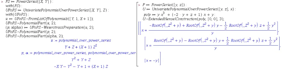
coincides with the Newton-Puiseux algorithm, thus computing the Puiseux parametrizations of a plane curve about a point; this functionality is at the core of theLimitPointscommand of theRegularChainslibrary for computing limit points of quasi-components of the regular chains of dimension one. Note that the latter command can be used in two different flavors
LimitPoints(R,coe f f icient = real) and LimitPoints(R,coe f f icient = complex), where the argumentcoefficientis used to indicate the coefficient ring for computing limit points corresponding to input regular chain R. For the case of a univariate polynomial with multi-variate polynomial coefficients, the EHC is a weak version of Jung-Abhyankar Theorem9. The commandExtendedHenselConstructionof the sub-package UnivariatePolynomialOver-PowerSeriesin thePowerSerieslibrary provides this latter flavor of the EHC.
2.3
The problem and related work
In regular chain theory, one desirable and challenging objective is, given a regular chainR, to obtain the (non-trivial) limit points of its quasi-componentW(R), or equivalently, computing the variety of its saturated ideal sat(R). The set lim(W(R)) of the non-trivial limit points of W(R) satisfiesV(sat(R))= W(R) = W(R) ∪ lim(W(R)). Hence, lim(W(R)) is the set-theoretic difference V(sat(R))\W(R). Deducing lim(W(R)) or V(sat(R)) from R is a central question which has theoretical applications (like the so-called Ritt Problem) and practical ones (like removing redundant components in triangular decomposition, or tangent cone computation).
In this thesis, the main problem we are facing is computing limit points corresponding to a regular chain. Up to our knowledge, the only way to compute limit points, is via a method based on Gr¨obner basis theory, using the well-knownRabinowitsch trick, seehttps://en. wikipedia.org/wiki/Rabinowitsch_trick(as of May 2017).
This latter method, when applied to the computation of sat(R) does not take the advantage of the triangular structure of the regular chainR. Therefore, it is desirable to consider a method well-adapted to regular chains. Moreover, one may wonder whether it is possible to compute
7See the wikipedia pagehttps://en.wikipedia.org/wiki/Weierstrass_preparation_theorem, as
of May 2017.
8For Hensel Lemma, see the wikipedia pagehttps://en.wikipedia.org/wiki/Hensel%27s_lemma, as
of May 2017.
9See this page from MathOverflow https://mathoverflow.net/questions/92618/
lim(W(R)) in polynomial time with respect to the degrees and coefficient heights of our input regular chainR.
Our method for computing lim(W(R)), when sat(R) has dimension 1, see Chapter 4, relies on a theorem of D. Munfored [70], which relates the closures of a constructible set in the Euclidean and Zariski topologies. One the problem is transported in the Euclidean topology, one canPuiseux series expansions, see [63, 2].
Initially, our implementation of theLimitPointscommand was built uponMaple’salgcurve
package, which implements Newton-Puiseux’s algorithm. But, as we wanted to factor poly-nomials over multivariate Puiseux series rings, we had to switch to the EHC. And since no implementation of the EHC is available inMaple, we had to realize our own, which was the original motivation for developing thePowerSerieslibrary10.
The EHC was originally introduced in [82] by Sasaki and Kako. Their work was further extended by their students in [47, 81, 48, 46, 83]. In [3], and thus in Chapter 3, we present tech-niques enhancing the EHC as well as complexity estimates for its main sub-routines. In [51], Kung and Traub also present a complexity analysis for Newton-Puiseux algorithm over the fieldC of complex numbers. Considering that EHC method computes all the branches while
Newton-Puiseux algorithm computes only one branch among the conjugate branches, our com-plexity results matches theirs, up to some log factors.
Returning to the problem of computing limit points of quasi-components of regular chains, we have also taken another approach to address this problem, by using changes of coordinates, see [4] and Chapter 6. This work not only focuses on computing limit points but also tries studying regular chains under changes of coordinates specially N other normalization. For more details on N¨other normalization, see books [39, 34] and papers [84, 43].
Turning our attention now to applications of limit point computations, we discuss tangent cones of space curves. Tangent cone computations can be approached at least in two ways. First, one can consider the formulation based on homogeneous components of least degree, see Definition 21. The original algorithm of Mora [65] follows this point of view. Secondly, one can consider the more “intuitive” characterization based on limits of secants, see Lemma 31.
As it was mentioned in Chapter 1, parametric representations of algebraic curves and sur-faces are used in Computer Aided Geometric Design. However, working with parametric rep-resentation instead of the implicit reprep-resentation bring its own challenges, in particular the problem of determining missing points. One way of dealing with this problem is to find, when it exists, a parametrization that covers the whole curve or surface, or, in other words, anormal parametrization. In the case of a curve, this problem is solved in [85], while it remains open for algebraic surfaces. An alternative approach, taken in [12], [86], and [87] is to compute finitely many parametric representations to cover all the points on the surface.
Another interesting application of computing limit points of quasi-components of regular chains is computing the limit of fractions of multivariate polynomials. Computing limits of such functions is a basic task in multivariate calculus and different mathematical concepts are defined based on these limits. The case of univariate analytic functions, including transcen-dental ones, has been well studied [40, 41, 80] and the corresponding algorithms are available in popular computer algebra systems. In calculus, we learned how to useL’hospital’s rule in order to compute the limit of univariate functions. In [54] by G.R. Lawlor, a generalization of
2.3. The problem and related work 25
L’hospital’s rulehas been developed for computing the limit of multivariate functions in some special cases. Surprisingly, the limit computations of multivariate functions is still an active research area.
In [104] S.J. Xiao and G.X. Zeng proposed a first algorithm that, given a multivariate rational function q ∈ Q(x1, . . . ,xn), decides whether lim(x1,...,xn)→(0,...,0)q is zero or not. The “not-case” includes the situation where lim(x1,...,xn)→(0,...,0)q does not exist as well as the case where it exists but it is not zero.
In [21], C. Cadavid, S. Molina and J.D. V´elez proposed an algorithm, now available in Maple as the limit/multi command, for determining the existence and possible value of
limits of the form lim(x,y)→(0,0)q, where q is a bivariate rational function, and such that (0,0)
is an isolated zero of the real algebraic set defined by the denominator ofq. In a follow-up preprint [98], J.D. V´elez, P. Hern´andez and C. Cadavid extend the method of [21] to rational functions in three variables, still assuming that the origin is an isolated zero of the denominator. Both papers [21] and [98] rely on the key observation that, for determining the existence and possible value of limits of the form lim(x,y)→(0,0)q and lim(x,y,z)→(0,0,0)q, it is sufficient to
studylimits along a real algebraic setχ(q), that is, limits of the form lim(x,y)→(0,0),(x,y)∈χ(q)qand
lim(x,y,z)→(0,0,0),(x,y,z)∈χ(q)q.
The method of S.J. Xiao and G.X. Zeng [104] has the advantage of not making any assump-tions on the number of variables nor the zero set of the denominator. Meanwhile, the works of C. Cadavid, S. Molina, J.D. V´elez and P. Hern´andez avoid the use of infinitesimal elements and rely on a deeper geometrical insight, through a notion of discriminant variety; unfortu-nately, the recourse to singular loci and irreducible decomposition is a limitation in view of an implementation of the method proposed in [21].
In [8], we have proposed an algorithm for determining the existence and possible value of
lim(x1,...,xn)→(0,...,0)q, for an arbitrary numbernof variables. As in [21] and [98], we assume that
the origin is an isolated zero of the denominator of the rational functionq. However, we avoid the computation of singular loci and the decomposition into irreducible components of the real and complex algebraic sets involved in the method. Instead, we take advantage of the theory of regular chains and theRealTriangularizealgorithm [23, 22] for decomposing semi-algebraic systems.
The experimental results reported in Section 6 of [8], suggest that our algorithm can solve more problems than the algorithm of S.J. Xiao and G.X. Zeng, in particular when the number of variables increases.
Chapter 3
Extended Hensel Construction
3.1
Introduction
The Extended Hensel Construction(EHC) is an algorithm which is used for factorizing uni-variate polynomials with power series coefficients. It was proposed in [82] by T. Sasaki and F. Kako. Their goal was to provide a practically more efficient alternative to the classical Newton-Puiseux method for univariate power series coefficients. In the same paper, Sasaki and Kako proposed an extension of the EHC to power series coefficients in more than one variable. Figure 3.1 illustrates our implementation of the EHC in thePowerSerieslibrary, available at
www.regularchains.org.
Figure 3.1: EHC applied to a trivariate polynomial.
The work of Sasaki and Kako was further extended by their students, see the papers [47, 81, 48, 46, 83]. See also the works of S. Abhyankar [1] and T.-C. Kuo [52]. The EHC relies on the so-calledYun-Moses polynomialsoriginally introduced in [69], studied in [94], and called Lagrange interpolation polynomials in [82]. The definition of those polynomials suggests to compute them by applying the Extended Euclidean Algorithm (EEA) over a field of multivari-ate rational functions. In practice, this is a computational bottleneck. In [81], Sasaki and D. Inaba suggest to use Gr¨obner bases instead and report on favourable experimental results.
In this chapter, we propose a new method for computing the Yun-Moses polynomials using Wronskian matrices. For an input bivariate polynomial F(X,Y) with coefficients in a field