Specific Emitter Identification via Feature Extraction
in Hilbert-Huang Transform Domain
Zhiwen Zhou1, 2, *, Jingke Zhang1, and Taotao Zhang3
Abstract—Aimed at the deficiency of conventional parameter-level methods in radar specific emitter identification (SEI), which heavily rely on empirical experience and cannot adapt to the waveform change, a novel algorithm is proposed to extract specific features and identify in Hilbert-Huang transform domain. Firstly, 2-dimensional physical representation of emitters is formed with Hilbert-Huang transform (HHT). Based on this, 4 types of multi-view features are constructed, and the feature space is spanned by elaborating the extraction. Principal components, between-class similarity, spectrum entropy, and deep architecture are used to describe the subtle features. Finally, support vector machine (SVM) is selected as the classifier to realize identification to alleviate the small sample problem. Experimental results show that the proposed algorithm realizes specific identification using 4 intentional modulations of simulated data. The selected 4 types of unintentional representations are feasible to discriminate identical emitters. Additionally, the proposed algorithm obtains higher accuracy than typical signal-level methods in the signal-to-noise ratio (SNR) range [0,20] dB.
1. INTRODUCTION
Specific emitter identification (SEI), also called fingerprint identification, aims at extracting fingerprint information after interception and deleaving, then determining the identical property of radar emitters by comparing with prior knowledge in database. The foundation of SEI is the unintentional modulation caused by manufacturing error and unavoidable device difference. With the complexity of electromagnetic environment, conventional SEI methods based on pulse parameters, such as radio frequency (RF), pulse width (PW), pulse recurrence interval (PRI), cannot meet the demands of precise identification at present [1]. Besides, military requirement of SEI technology is urgently increasing. To execute SEI, the fingerprint features should satisfy five criteria, namely, generality, uniqueness, stabilization, measurability, and independence. Based on this, emitters from the identical type of radars but in different platforms can be distinguished.
According to the literature at present, SEI methods have been researched in two directions, parameter-level and signal-level. The former focuses on time or frequency domain. They heavily rely on empirical design, which results in reassessment when platforms or modulations change. Intuitive systemic model [2] is established to effectively describe and explain the fingerprint features. Generally, pulse feature [3], frequency-domain distribution [4, 5], and unintentional phase modulation [6] are selected as unintentional representations. However, parameter-level methods require stringent design for model establishment and feature selection. Especially, the applicability needs to be validated with practical data. In comparison, signal-level methods have the advantage of comprehensive description. Various features and combinations are presented to perform signal-level SEI, although the mechanism has not been explained theoretically. High-order cumulants [7], wavelet ridge and high order spectra [8],
Received 25 February 2019, Accepted 14 June 2019, Scheduled 28 June 2019
* Corresponding author: Zhiwen Zhou (mini [email protected]).
bispectrum and its variants [9–11] have demonstrated the effectiveness for the given conditions. Recently, Hilbert-Huang transform (HHT) has proven the superiority in the unique representation and descriptive ability for SEI [12–15]. It provides an accurate amplitude distribution with the change of time and frequency, but does not need the prior information about the analyzed signal. Additionally, empirical mode decomposition (EMD) as the kernel in HHT is taken to extract meaningful features [16, 17]. Considering the advantages of HHT and aiming at SEI with multiple intentional modulations at low SNRs, a novel algorithm based on unintentional features in HHT-domain is proposed. First, radar emitters with unintentional modulations are analyzed with HHT. Then, 4 types of features in HHT distribution are put forward to describe the subtle discrimination. Finally, SVM is introduced as the classifier to achieve SEI.
2. SIGNAL MODEL
In general, considering the difference of transmitting devices, stochastic and deterministic distortions in the receiving channel, the intercepted emitters with unintentional modulation on pulse (UMOP) can be formulated as [4],
sd(t) =s(t) [1 + Δεa(t)] exp [jΔεp(t)] +n(t) (1)
where s(t) = A(t) exp[j2πfct+jc(t)] is the ideal received emitter without UMOP; A and fc are the pulse amplitude and carrier frequency, respectively; c(t) and n(t) are the phase modulation and noise functions; Δεa(t) and Δεp(t) denote the distortion functions of UMOP in amplitude and phase. Furthermore, Δεa(t) and Δεp(t) are assumed as follows,
Δεa(t) = εacos2πfat+kaπt2 (2)
Δεp(t) ∼ N (μf, kffc) (3)
whereεa,fa,ka,μf, andkf are the distortion coefficients of Δεa(t) and Δεp(t), respectively; N denotes
the normal distribution. To further realize identification reliably, the outliers and errors should be measured to simulate the practical environment.
3. FEATURE EXTRACTION IN HHT DOMAIN 3.1. HHT of Radar Emitter
Generally, HHT includes EMD and Hilbert spectrum analysis [13, 14]. EMD decomposes any signal into finite intrinsic mode functions (IMFs), and the decomposition bases are adaptively generated
0.5 1 1.5 2 2.2 3 3.5 4 4.5 5 -0.8
-0.6 -0.4 -0.2 0 0.2 0.4 0.6 0.8 1
No
rm
alize
d am
plit
ude
Time/µs
Original Normalized
0.5 1 1.5 2 2.5 3 3.5 4 4.5 5 -0.8
-0.6 -0.4 -0.2 0 0.2 0.4 0.6 0.8 1
No
rm
alized
a
m
p
li
tude
Time/µs
Original Normalized
(a) (b)
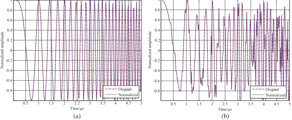
according to the original signal [16, 17]. The latter part implements Hilbert transform for each IMF. Due to the unintentional disturbance in amplitude and phase, extreme points in EMD process are difficult to calculate mathematically. Take linear frequency modulation (LFM) as the typical example and c(t) = 1/2πμt2, where μ is frequency modulation ratio. Then, Figs. 1(a) and (b) illustrate the original and reconstruction emitters after EMD with UMOP when SNR = 5 dB. SNR is defined as SNR = 10 log(σs2d/σ2n), whereσ2sd and σn2 are the average signal power and noise variance, respectively. By comparison, the original emitter can be approximately recovered via EMD. It demonstrates no information loss in time-domain, which shows excellent decomposition ability.
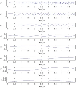
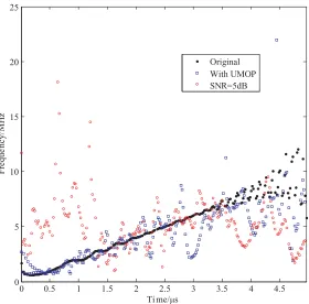
Figure 2 gives the decomposed IMFs of LFM with UMOP. Seen fromc1 ∼c8, the IMF components can adaptively track the change of emitter, which demonstrates the frequency properties. To exactly analyze the emitter, only using IMFs is inadequate to realize identification. Therefore, it is necessary to obtain HHT distributionH(ω, t)∈RT1×T2 to further extract the features. It can be seen from Fig. 3 that HHT time-frequency distribution of LFM has good accumulation ability, which approximately shows linear trend. However, frequency scatters with time while UMOP or noise exists. Consequently, it is not advisable to directly use H(ω, t) as the feature input, and further research should be taken to exploit unique representations.
c1
c2
c3
c4
c5
c6
c7
0 0.5 1 1.5 2 2.5 3 3.5 4 4 .5
- 2 0 2
Time/µs
0 0.5 1 1.5 2 2.5 3 3.5 4 4 .5
- 2 0 2
Time/µs
0 0.5 1 1.5 2 2.5 3 3.5 4 4 .5
- 1 0 1
Time/µs
0 0.5 1 1.5 2 2.5 3 3.5 4 4 .5
- 0.5 0 0.5
Time/µs
0 0.5 1 1.5 2 2.5 3 3.5 4 4 .5
- 0.5 0 0.5
Time/µs
0 0.5 1 1.5 2 2.5 3 3.5 4 4 .5
- 0.5 0 0.5
Time/µs
0 0.5 1 1.5 2 2.5 3 3.5 4 4 .5
- 0.05 0 0.05
Time/µs
0 0.5 1 1.5 2 2.5 3 3.5 4 4 .5
0 0.01 0.02
Time/µs
c8
Figure 2. Decomposed IMFs of LFM when SNR = 5 dB.
3.2. Feature Extraction
0 0.5 1 1.5 2 2.5 3 3.5 4 4.5 0
5 10 15 20 25
Ti me/µs
Fre
q
ue
nc
y/
MH
z
Original With UMOP SNR=5dB
Figure 3. Time-frequency distribution of Hilbert spectrum of LFM.
convolutional neural network (CNN) features. Especially, PCs stand for principal energy of time-frequency accumulation. CC aims to distinguish emitters by Hilbert spectrum resolution. SEn measures the distribution information in terms of frequency subband. CNN, or called deep feature, is to construct deep representations to capture the subtle difference. The proposed 4 features construct a relatively complete feature space from multi-view descriptions. Before computing the features,H(ω, t) is converted into a 2-dimensional greyscale image [12].
3.2.1. PCs
On the plane of H(ω, t), there exists subtle difference in instantaneous representation. Hence, it is advisable to directly process Hilbert spectrum in order to maintain information at utmost. We extract the principal components of Hilbert spectrum, which represent the principal energy on the plane. Since UMOP in Eq. (1) is mixed with the intentional signal, as shown in Fig. 3, the unavoidable but unique feature caused by UMOP is hidden in the distribution. Take singular value decomposition (SVD) on
H(ω, t) [18],
H=UΣVT (4)
whereΣ= [ Σ01 00 ] andΣ1 = diag(σ1, . . . , σr), the order of diagonal elements isσr≥σr−1≥. . .≥σ1; r is the rank of H,r = rank(H). Then, xPCs = [σr, σr−1, . . . , σ1] denotes the principal component of
H(ω, t). Since r depends on the rank, and minor components contribute little, we take 90% energy from principal components. Then, it yieldsxPCs= [σr, σr−1, . . . , σt], wheretis the maximum subscript
when the energy of the counted components is equal to 0.9.
3.2.2. CC
theith and jth Hilbert matrices, CC between Hi and Hj is defined as [12],
ρ(i,j) =
+mn(Hi,m,n−E[Hi]) (Hj,m,n−E[Hj])
(ΣΣ (Hi,m,n−E[Hi])) (ΣΣ (Hj,m,n−E[Hj])) (5) where Hi,m,n(Hj,m,n) is the (m, n) element of Hi(Hj). Eq. (5) measures the relevance between Hi
and Hj, which means that ρ(i,j) is large if Hi and Hj are from identical emitters. Otherwise, ρ(i,j) approximates 0. ChooseC2
n coefficients to form the feature vectorxCC = [ρ(1,2), . . . , ρ(n−1,n)].
3.2.3. SEn
SEn aims to describe the homogeneity of Hilbert time-frequency distribution in terms of information, which only depends on the distribution. First, 2-dimensional H(ω, t) is divided into several subbands {Hi(ω, t), i= 1, . . . , Nω}, whereNω is the subband number of frequency resolution Δω. Then, SEn of each subband is PSEn,i=
Hi(ω, t)dt. ForNω subbands, SEn can be calculated as [19],
xSEn=−
Nω
i PSEn,iln (PSEn,i) ln (Nω) (6)
It is worth noting that SEn varies with the certain frequency component. In the extreme circumstance,
xSEn approximates 0 with uniform time-frequency distribution. However, SEn will increase for the uncertainty and unpredictability caused by unintentional frequency turbulence. The turbulence includes the aforementioned UMOP.
3.2.4. CNN
Instead of picking out statistical features on H(ω, t), we use the typical deep learning architecture CNN to automatically extract feature and seek the subtle difference. CNN is composed of four layers, convolutional, activation, pooling, and full-connected layers. First, H(ω, t) is taken as the input to be convolved with convolutional layers and mapped with activation function. Down sampling is implemented to reduce the feature size. Then, the output feature maps are concatenated to form the feature representation xCNN. Training is conducted by minimizing the loss function with stochastic gradient descent (SGD). xCNN can be formulated as [20],
xCNN= vec [pool (f(H⊗C+b))] (7)
where C and b are the convolutional kernels and biases; f(·) is selected as the sigmoid function
f(x) = 1/(1 +e−x);⊗denotes the valid convolution; pool(·) and vec(·) are the pooling and vectorization operations, respectively. Generally, a series of convolutional layers are connected to produce deeper and more abstract features.
3.3. Identification
Considering the interception probability and interference, the available training samples are limited. The small sample problem will lead to under-fitting and degrade the identification performance. Therefore, SVM classifier is introduced to alleviate the problem. Given N training samples, features are then extracted as described in the previous subsection {xi,Yi}Ni=1, where xi is the selected feature, Yi the class label, andC=Yi the class number. SVM is intended to seek the optimum plane in the feature space, which can be converted to solve the discriminant as [13],
w,Φ (x)+bl= 0 (8)
where w and bl are the weights and offset of SVM; Φ(·) is the nonlinear function; · denotes the inner product. Once the optimal solution of Eq. (8) is obtained by quadratic programming [21], the identification for each feature can be implemented as,
Ypre= sign
Ns
i YiΦ (xi) Φ (xpre) +b ∗
l (9)
where xpre and Ypre are testing sample and label, respectively; Ns is the number of support vectors;
3.4. Discussions
The complexity of the proposed algorithm consists of three parts, the calculations of HHT and four features, and SVM classifier. The computation complexities of HHT and SVM can refer to [12]. Then, the complexity of PCs lies in Eq. (4), which is O(N T13). CC mainly depends on Eq. (5), which is O(N2T
1T2). For SEn, it is O(N NωT1T2). However, the whole complexity of CNN feature is O(NDl=1MlKlCl−1Cl), where D is the depth; Ml and Kl are the size of output feature map and kernel; Cl is the convolutional kernel number oflth layer.
Currently, the HHT-based methods have gained positive results. [12] uses the statistical characteristics of HHT spectrum distribution, such as energy entropy and second-order moment. The proposed features are vulnerable to the outliers and noise. However, the proposed HHT-UF constructs more diverse descriptions; for example, CNN feature is deep and automatic, and SEn is more practical via information representation when unintentional turbulence exists. Moreover, the proposed method provides more detailed features than parameter-level methods.
4. EXPERIMENTAL RESULTS AND ANALYSIS
To testify the effectiveness and robustness, simulated emitters are generated according to Eqs. (1)–(3), and the parameters are set as follows, εa = 0.2, fa = 1000 MHz, ka = 105MHz, μf = 0, kf = 0.001, fc = 10 MHz. To evaluate the adaptability to the modulations, four types of radar emitters are selected, namely conventional pulse (CON), LFM, binary frequency-shift keying (BFSK), and binary phase-shift keying (BPSK). Random turbulence is added according to Eqs. (2)–(3), and the explicit parameter setting is listed. Each type with the turbulence generates 300 samples at SNR = 30 dB, which amounts to 4800 samples. The Hilbert spectrum size is 200×250. Radial based function (RBF) is chosen for SVM classifier, and its toolbox can refer to [21].
4.1. Effectiveness Experiment
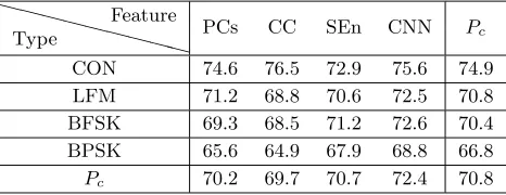
To testify the effectiveness, 100 testing samples for each modulation is generated in AWGN channel with SNR = 6 dB. Each feature is input into SVM separately. The performance is measured by the probability of correct identification Pc. The experimental results in Table 1 show that the average
Pc of all the features is approximately larger than 70%. Meanwhile, the average performance for the given modulations is around 70%. But they differ from each other, which attributes to the difference of feature representations. In comparison, CNN is more distinguished than the other features. It shows that seeking the difference in data structure essentially helps to prompt the performance.
Table 1. SEI probabilities with different features at SNR = 6 dB. XXXXXType XXXXFeature PCs CC SEn CNN P
c
CON 74.6 76.5 72.9 75.6 74.9
LFM 71.2 68.8 70.6 72.5 70.8
BFSK 69.3 68.5 71.2 72.6 70.4
BPSK 65.6 64.9 67.9 68.8 66.8
Pc 70.2 69.7 70.7 72.4 70.8
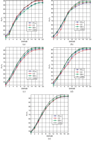
4.2. Robustness Experiment
0 2 4 6 8 10 12 14 16 18 20 55 60 65 70 75 80 85 90 95 SNR/dB Pc /% PCs CC SEn CNN
0 2 4 6 8 10 12 14 16 18 20
50 55 60 65 70 75 80 85 90 95 SNR/dB Pc /% PCs CC SEn CNN
0 2 4 6 8 10 12 14 16 18 20 50 55 60 65 70 75 80 85 90 SNR/dB Pc /% PCs CC SEn CNN
0 2 4 6 8 10 12 14 16 18 20 45 50 55 60 65 70 75 80 85 90 SNR/dB Pc /% PCs CC SEn CNN
0 2 4 6 8 10 12 14 16 18 20 50 55 60 65 70 75 80 85 90 SNR/dB Pc /% PCs CC SEn CNN (a) (b) (c) (d) (e)
that the accuracies rise with increasing SNR. In comparison, BPSK with UMOP is less discriminable for the unintentional phase modulation feature is easily affected and hard to capture. The average does not show distinct advantage over the single feature. It can be seen that CNN feature in HHT domain shows relative superiority. Hence, it is not preferable to combine the proposed 4 features in consideration of computing complexity. When SNR ≥ 2 dB, the identification probabilities of the 4 features are over 50%. Then,Pc rises until SNR is close to 18 dB, when it maintains stable. It indicates that higher SNR
contributes a little to the performance and implies tha tSNR is not the decisive factor now.
Aimed at SEI, typical high-order cumulant [8], bispectrum [9], and SOM [12] all prove to be effective. Then, the proposed HHT-UF is compared with the listed approaches. Keep all the setting parameters the same. The aforementioned 4 types of emitters are used, and the average Pc is served as the performance measurement. HOSA toolbox in Matlab is directly used to analyze bispectrum and high-order cumulant. Especially, the compared methods all belong to signal-level. The results in Fig. 5 show that Pc of HHT-UF is higher than the others for the given SNR range. On one hand, UMOP feature representation in HHT domain is beneficial for the subtle discrimination. On the other hand, the overall performance of multi-dimensional features show the advantage over the single feature. However, the computation complexity increases accordingly. Therefore, it is advisable to speed up the HHT-UF algorithm for further research and use it in ESM and ELINT where real-time demand is not strict.
40 45 50 55 60 65 70 75 80 85 90 95
0 2 4 6 8 10 12 14 16 18 20
[8] [9] [12] HHT-UF
Figure 5. SEI probabilities of different methods with SNR∈[0,20] dB.
5. CONCLUSIONS
Aimed at the deficiency of conventional parameter-level SEI methods, a novel signal-level algorithm that realizes UMOP feature extraction, and identification in HHT domain is proposed. Radar emitters are modeled with unintentional frequency and phase modulations. Then, features are described and extracted via EMD and Hilbert spectrum. SVM is chosen as the classifier to avoid small sample problem. The validation is testified with the established model and four modulations of simulation data. Experimental results show that the proposed features are effective and robust to addictive Gaussian noise. The multiple-dimension features help to promote the identification, but leads to a corresponding increase in computation burden. Since UMOP phase feature is susceptible to the outliers and noise, SEI modeling for radar emitter with phase modulation needs further investigation.
REFERENCES
2. Han, T. and Y. Y. Zhou, “Intuitive systemic models and intrinsic features for radar-specific emitter identification,” Foundations and Practical Applications of Cognitive Systems and Information Processing, Vol. 215, 153–160, 2014.
3. Conning, M. and F. Potgieter, “Analysis of measured radar data for specific emitter identification,”
IEEE Radar Conference, 35–38, IEEE Press, New York, 2010.
4. Ru, X. H., Z. T. Huang, Z. Liu, et al., “Frequency-domain distribution and bandwidth of unintentional modulation on pulse,”Electronics Letters, Vol. 52, No. 22, 1853–1855, 2016.
5. Ru, X. H., Z. Liu, Z. T. Huang, et al., “Evaluation of unintentional modulation for pulse compression signals based on spectrum asymmetry,” IET Radar, Sonar and Navigation, Vol. 11, No. 4, 656–663, 2017.
6. Ye, H., Z. Liu, and W. Jiang, “Comparison of unintentional frequency and phase modulation features for specific emitter identification,” Electronics Letters, Vol. 48, No. 14, 875–877, 2012. 7. Aubry, A., A. Bazzoni, V. Carotenuto, et al., “Cumulants-based radar specific emitter
identification,” 2011 International Workshop on Information Forensics and Security, 1–6, IEEE Press, New York, 2011.
8. Ren, M. Q., J. Y. Cai, Y. Q. Zhu, et al., “Radar signal feature extraction based on wavelet ridge and high order spectra analysis,”IET International Radar Conference, 1–5, IEEE Press, New York, 2009.
9. Liang, K. Q., Z. Huang, D. X. Hu, et al., “An individual emitter recognition method combining bispectrum with wavelet entropy,” International Conference on Progress in Informatics and Computing, 206–210, IEEE Press, New York, 2015.
10. Ding, L. D., S. L. Wang, F. G. Wang, et al., “Specific emitter identification via convolutional neural networks,”IEEE Communications Letters, Vol. 22, No. 12, 2591–2594, 2018.
11. Kang, N. X., M. H. He, J. Han, et al., “Radar emitter fingerprint recognition based on bispectrum and SURF feature,”2016 CIE International Conference on Radar, 1–5, Guangzhou, 2016.
12. Zhang, J. W., F. G. Wang, O. A. Dodre, et al., “Specific emitter identification via Hilbert-Huang transform in single-hop and relaying scenarios,”IEEE Transactions on Information Forensics and Security, Vol. 11, No. 6, 1192–1205, 2016.
13. Yuan, Y. J., Z. T. Huang, H. Wu, et al., “Specific emitter identification based on Hilbert-Huang transform-based time-frequency-energy distribution features,”IET Communications, Vol. 8, No. 13, 2404–2412, 2014.
14. Hui, X. N., S. L. Zheng, J. H. Zhou, et al., “Hilbert-Huang transform time-frequency analysis in φ-OTDR distributed sensor,” IEEE Photonics Technology Letters, Vol. 26, No. 23, 2403–2406, 2014.
15. Han, J., T. Zhang, Z. Y. Qiu, et al., “Communication emitter individual identification via 3D-Hilbert energy spectrum-based multiscale segmentation features,” International Journal Communication System, Vol. 32, No. 1, e3833, 2019, https://doi.org/10.1002/dac.3833.
16. Zhu, B. and W. D. Jin, “Feature extraction of radar emitter signal based on wavelet packet and EMD,” Information Engineering and Applications, Vol. 7, No. 6, 198–205, 2012.
17. Liang, J. H., Z. T. Huang, and Z. W. Li, “Method of empirical mode decomposition in specific emitter identification,” Wireless Personal Communications, Vol. 96, No. 3, 2447–2461, 2017. 18. Guo, Q., P. L. Nan, X. Y. Zhang, et al., “Recognition of radar emitter signals based on SVD and
AF main ridge slice,” Journal of Communications and Networks, Vol. 17, No. 5, 491–498, 2015. 19. Zhang, G. X., H. N. Rong, L. Z. Hu, et al., “Entropy feature extraction approach for radar emitter
signals,” International Conference on Intelligent Mechatronics and Automation, 621–625, IEEE Press, New York, 2004.
20. Zhou, Z. W., G. M. Huang, H. Y. Chen, et al., “Automatic radar waveform recognition based on deep convolutional denoising auto-encoders,”Circuits, Systems, and Signal Processing, Vol. 37, No. 9, 4034–4048, 2018.
![Figure 5. SEI probabilities of different methods with SNR ∈ [0, 20] dB.](https://thumb-us.123doks.com/thumbv2/123dok_us/1968638.1259724/8.612.151.466.310.473/figure-sei-probabilities-dierent-methods-snr-db.webp)
