Scholarship@Western
Scholarship@Western
Electronic Thesis and Dissertation Repository
6-6-2017 12:00 AM
Dynamic Functional Connectivity Reveals Temporal Differences in
Dynamic Functional Connectivity Reveals Temporal Differences in
Wake and Stage-2 Sleep
Wake and Stage-2 Sleep
Mazen El-BabaThe University of Western Ontario Supervisor
Dr. J Bruce Morton
The University of Western Ontario Joint Supervisor Dr. Adrian Owen
The University of Western Ontario Graduate Program in Neuroscience
A thesis submitted in partial fulfillment of the requirements for the degree in Master of Science © Mazen El-Baba 2017
Follow this and additional works at: https://ir.lib.uwo.ca/etd Part of the Cognitive Neuroscience Commons
Recommended Citation Recommended Citation
El-Baba, Mazen, "Dynamic Functional Connectivity Reveals Temporal Differences in Wake and Stage-2 Sleep" (2017). Electronic Thesis and Dissertation Repository. 4603.
https://ir.lib.uwo.ca/etd/4603
This Dissertation/Thesis is brought to you for free and open access by Scholarship@Western. It has been accepted for inclusion in Electronic Thesis and Dissertation Repository by an authorized administrator of
i
The transition from wakefulness to sleep is marked by changes in neurophysiology,
suggesting that changes in consciousness might be accompanied by changes in functional
network organization. Brain activity of 21 healthy participants was measured via simultaneous
EEG-fMRI as participants transitioned from wakefulness into sleep. All fMRI volumes were
ICA-decomposed, yielding 42 neurophysiological sources. Independent component time courses
were used to estimate mean functional connectivity (FC) and dynamic FC using a sliding
window technique. Windowed matrices were submitted to k-means clustering (k = 7, L2-norm).
Mean FC in Wake and Stage-2 Sleep (S2S) were similar. Dynamic analysis revealed differences
in temporal features of FC. Participants transitioned more between connectivity states (CSs) and
spent less time across all CSs in Wake than in S2S. Four of the seven CSs differed in their
frequencies. The current analysis suggests conventional FC analyses obscure features in FC that
are observable on a finer temporal scale.
Keywords
ii
Acknowledgments
Dr. J Bruce Morton: I would like to deeply thank Dr. J Bruce Morton for his sincere care,
thoughtfulness, supervision, and guidance. Dr. Morton, you have truly inspired me to strive for
the best. Your academic and personal integrity truly reflect on the type of scholar, supervisor,
and person you are. I am very fortunate to have had the opportunity to know you personally and
professionally.
Ahmad El-Baba, Aseel El-Baba, Hadeel El-Baba, and Mayssa El-Bizri: your names were written
alphabetically, so please do not complain about your position on the list. You are all always there
for me no matter what. I could have never asked for a more supportive and loving family. You
all mean so much to me. Mayssa and Hadeel, thank you for trying to listen to my talks. I know it
probably felt like torture; but your willingness to hear them out means a lot to me. Aseel, you
tried; and trust me, I understand that sleep is more important! Thank you for always pushing me
to pursue my dreams. Also, I would like to send my special thanks to my mother, Mayssa, who
was extremely helpful and supportive during the H.appi Camp. Without your help and support in
everything I do, this Master’s degree would not be possible.
Niki and Nellie Kamkar: thanking you for your love and care will never, ever, be enough. You
were always there to make sure that my rainy days became sunny (with no chance of clouds).
Niki, thank you for the countless phone calls, random conversations, and advice. I always know
that you have my back no matter what. I believe that I gained amazing colleagues, life-long
iii
Samantha Faith Goldsmith (SFG): My gut instinct almost never fails me… but I guess I have to
admit, it did once! I am so grateful that you joined our lab in 2016. I can endlessly talk to you
about anything! You were really my sanity check towards the end of my Master’s journey. You
were always there at the lab, and I was always happy to see you there! Sorry for placing you on
the corner-desk of the lab!
Daniel J Lewis: I will never forget our long nights at the lab and our never-ending white-board
drawings and discussions. You taught me so much in the past year and a half. I would still be
fighting MATLAB right now if it was not for your generous help and patience!
Bea Goffin: I will deeply miss our “Bea chats”. You have supported me in every step of the way.
I can always walk in your office and spill my heart out knowing that you will be there to listen
and support me in any way you can. For that, I thank you deeply!
Dr. Adrian Owen, Dr. Andrea Suddo, and Dr. Stuart Fogel: Thank you for your sincere care and
for taking the time to advise me throughout my time at Western. I found our conversations
extremely stimulating and enjoyable!
Dr. Stuart Fogel, Laura Ray, Lydia Fang, and Max Silverbrook: Thank you all very much for all
your help. Our sleepless nights at the sleep lab (ironic) will never be forgotten!
iv
Table of Contents
Abstract ... i
Acknowledgments ... ii
List of Figures ... vi
1.0 Introduction ... 1
1.1 A Historical Overview ... 1
1.1.2 Theological Account ... 1
1.1.1 Philosophical Account ... 2
1.2 Current Knowledge ... 3
1.3 Potential Caveats ... 6
2.0 Methods... 8
2.1 Participants ... 8
2.2 Experimental Procedure ... 9
2.3 Data Acquisition and Preprocessing ... 9
2.4 Group ICA and Post-Processing ... 12
2.5 Stationary Mean FC Estimation ... 15
2.6 Dynamic FC Estimation ... 15
2.6 Dynamic Metrics ... 18
2.7 Reliability of Connectivity States and Dynamic Metrics ... 19
2.8 Estimating Heart Rate ... 19
3.0 Results ... 20
3.1 Stationary Mean FC ... 20
3.2 Dynamic FC ... 21
v
3.2.2 Mean Dwell Time ... 22
3.2.3 Reliability of Connectivity States and Dynamic Metrics ... 25
3.2.4 Temporal Characteristics of FC ... 28
3.2.5 Transition Probabilities ... 30
3.3 Heart Rate ... 31
4.0 Discussion ... 31
4.1 Mean vs. Dynamic FC ... 31
4.2 Theoretical Accounts ... 33
4.3 Connectivity States ... 35
4.4 Limitations ... 37
4.4.1 Stationary Analysis ... 37
4.4.2 Dynamic Analysis ... 38
4.4.3 Statistical Criteria ... 38
4.5 Concluding Remarks ... 39
References ... 40
vi
List of Figures
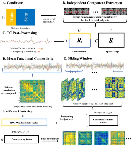
Figure 1. Step-by-step analysis steps are depicted in this figure. A, Subjects wake and sleep
volumes where organized and submitted to group-level spatial independent component analysis
(ICA). B, ICA was performed using the GIFT toolbox implemented in MATLAB; 42
neurophysiologically plausible sources were selected and sorted into functional families. GICA 1
back-reconstruction was used to estimate the time courses (Ri) and spatial maps (Si) for each
subject. C, All time courses (TCs) were post processed by removing subject motion variance,
despiking, and filtering. D, TCs were used to estimate mean FC in Wake and Stage-2 Sleep by
computing pairwise correlations between all ICs. E, As outlined by Allen et al., 2014, dynamic
FC was estimated using a sliding window approach (window width = 15 TRs, time step = 1 TR)
resulting in windowed correlation matrices. Correlation matrices were vectorized and
concatenated into a large data matrix of all IC-to-IC pairwise correlation values over time. All
windows were demeaned on a subject level by removing subject specific means from subject
windows in Wake and Stage-2 Sleep. The concatenated data matrix was submitted to k-means
clustering (F). k-means clustering was performed to extract recurrent features of the data. A k-7
solution was selected which resulted in a matrix with rows equivalent to the number of
connectivity states (7) and columns equivalent to the number of unique IC-IC correlations (861).
Each row representing a connectivity states was back-reconstructed into a matrix format to
visualize coupling relationships between ICs. An IDX vector, a window state label vector,
unique for each subject in Wake and Stage-2 Sleep was also computed revealing window
vii
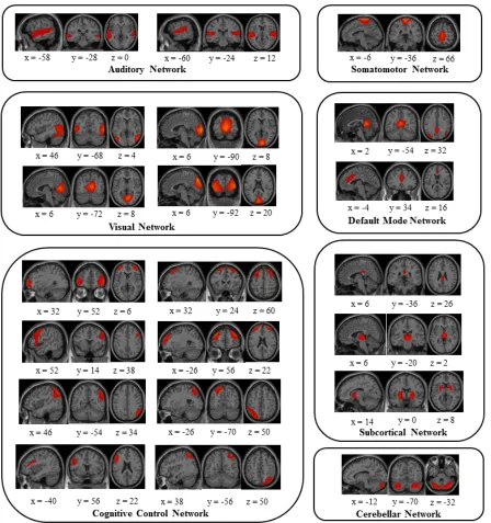
Figure 2. 42 neurophysiologically plausible independent components (ICs) were divided into
groups and arranged based on their spatial and functional properties. A total of seven functional
families were identified including the auditory, somatomotor, visual, default mode, cognitive
control (including the dorsal and ventral attention networks), subcortical, and cerebellar
networks. ICs are displayed on sagittal, coronal, and horizontal slices on a cortical surface
implemented in MANGO. ... 17
Figure 3. Mean functional connectivity in WAKE (A), and STAGE-2 Sleep (B). Each square
represents the coupling relationship between the IC on the x-axis and the IC on the y-axis. The
diagonal represents a perfect (r = 1.0) correlation between an IC and itself. Within defined
boundaries around the diagonal, positive correlations were found indicating strong coupling
relationships between ICs that were classified under the same functional family (e.g., ICs within
the Auditory network). Off-diagonally, weaker connectivity can be found between functional
families. ... 20
Figure 4. Stationary Mean FC in Wake (B) subtracted from stationary mean FC in Stage-2 Sleep
(A) to produce a Difference Matrix (C). t tests were performed with the null hypothesis of zero
correlation on the Difference Matrix (D). To correct for multiple comparisons, the false
discovery rate (FDR) method was used with a P value of .01. t-tests confirmed that mean FC in
Wake and Stage-2 Sleep were similar, as differences between the correlations in both conditions
were not significantly greater than 0. ... 21
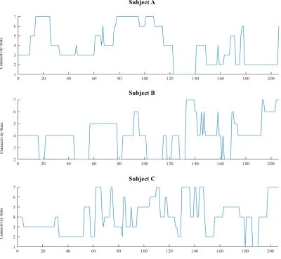
Figure 5. IDX vector of three representative participants during wakefulness. The number of
windows is on the x-axis and the connectivity state is on the y-axis. Plots illustrate transitions
viii
Figure 6. Clustering analysis revealed 7 connectivity states in Wake and Stage-2 Sleep (A). Each
square represents the coupling relationship between the IC on the x-axis and the IC on the y-axis.
B, mean frequency of state expression in Wake (yellow) and Stage-2 Sleep (blue). The frequency
of connectivity state-1 and 6 were significantly greater in Stage-2 Sleep (*, p < .05). The
frequency of connectivity state-5 was significantly greater in Wake (*, p < .05); the frequency of
connectivity state-4 expression in wake was marginally significant when compared to Stage-2
Sleep (#, p = .053). C, mean dwell time of the four connectivity states that had differences in
their frequencies of expression in Wake and Stage-2 Sleep. Mean dwell time was significantly
greater in Stage-2 Sleep than in Wake (*, p < .05). ... 24
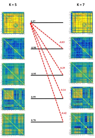
Figure 7. Spatial correlations comparing connectivity states from a k-5 solution and k-7 solution.
Black lines connect qualitatively similar connectivity states. Red dashed lines show the spatial
correlations of connectivity state-1 in a k-5 solution with connectivity states in a k-7 solution.
Weaker correlations are indicative of the robustness of the connectivity states in varying
k-solutions and the uniqueness of their spatial topologies. Spatial correlations were iteratively
computed between all connectivity states to confirm the similarity of selected connectivity states
across varying k-solutions. ... 26
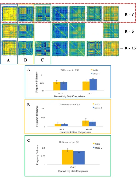
Figure 8. Difference scores were computed for connectivity states that showed statistically
significant differences in Wake and Stage-2 Sleep. Top three panels show the connectivity states
matrices derived from k-5, k-7, and k-15 solutions. The connectivity states were organized by
grouping, column-wise, qualitatively similar states. Each group is highlighted and labeled as A,
B, or C. Corresponding bar graphs are also labeled and highlighted with the same colour. The
frequency of expression for connectivity state-1 (A), connectivity state-5 (B), and connectivity
ix
bars represent the difference scores during Wake, and blue bars represent the difference scores in
Stage-2 Sleep. Frequency of expression did not change across k-solutions. This is indicative of
the robustness of the dynamics analysis across different k solutions. ... 27
Figure 9. Mean number of transition (NT) in Wake and Stage-2 Sleep. Participants’ NTs in
Wake and Stage-2 Sleep are transformed by dividing their NT by the length of their IDX vector.
Participants expressed more transitions in Wake than in Stage-2 Sleep (p < .05). ... 29
Figure 10. Mean inter-transition interval (average number of consecutive windows) in Wake and
Stage-2 Sleep. Y-axis represents the number of consecutive windows. The inter-transition
interval was significantly higher in Stage-2 Sleep than in Wake (p < .05). ... 29
Figure 11. Transition probabilities for Stage-2 Sleep and Wake shown. Matrices represent the
probability of transitioning from i-state on the y-axis to j-state on the x-axis. Darker yellow
squares in the Difference matrix represent a higher probability of transition in Stage-2 Sleep than
Wake, while darker blue squares represent a higher probability of transition in Wake than
Stage-2 Sleep. Probabilities in the difference matrix range from 0 to .10. ... 30
Figure 12. Mean heart rate (beats per minute) in Wake and Stage-2 Sleep. There was no
1.0
Introduction
1.1 A Historical Overview
1.1.2 Theological Account
Over the past centuries, many scholars, philosophers, and religious leaders asked
questions related to sleep. According to Middle Eastern folktales, sleep is an intermediate state
between wakefulness and death. It is regarded as the gateway for the living to interact with the
dead. These ideas are instantiated in religious scriptures that discuss the role of the soul in the
transition from wakefulness to sleep. In Islam, death and sleep are often discussed in the same
verses of the Qur’an (BaHammam, 2011). The holy book of Islam states that God (Allah) takes
the human soul permanently upon death, but retains the soul only temporarily during sleep
(BaHammam, 2011). It is said that the soul exits the body through a person’s navel, allowing the
soul to venture between the living and the dead. Accordingly, dreams that include alive and
deceased individuals are thought to be a result of the souls communicating with one another
during sleep. Because sleep is regarded as an intermediary stage, when the Prophet Mohammed
was asked if people sleep in Heaven, he answered: “sleep is the brother of death. People of
Heaven do not sleep” (BaHammam, 2011). His statement indicates that once a person is dead,
they will no longer be able to sleep because they will be living, awake, eternally in Heaven.
The comparison of sleep and death predates Islam as parallels are also drawn in the Old
and the New Testaments. Sleeping and dying appear to be synonymous in Christian Holy books.
reiterated his statement by saying “Lazarus is dead” (Jn. 11:14). Perhaps, sleep and death were
viewed under the same lens given the similarity of the body’s appearance in both states–
immobile and unaware. In Judaism, sleep is considered 1/60th of death. Like Muslims, Jews
believe that the soul is taken and cleansed by God during sleep, and is returned to the human
body upon wakefulness. For that reason, Jews and Muslims, alike, recite a prayer upon waking,
thanking God for restoring their souls. For example, the Jews say: “I offer thanks to You, living
and eternal King, for You have mercifully restored my soul within me; Your faithfulness is
great.”
1.1.1 Philosophical Account
Alcmaeon (450 BC) was one of the earliest Greek philosophers on record to propose that
the flow of blood from the skin to the core was essential in mediating the transition from
wakefulness to sleep, whereas the outward flow of blood towards the skin would result in
wakefulness (Papachristou, 2014). A century later (350 BC), Aristotle continued the quest to
unravel the mystery of sleep by proposing that sleep occurs during the process of digestion, and
ceases when digestion is complete (Papachristou, 2014). These philosophical ideas are indicative
of the dominant school of thought during ancient times that focused on the heart and the blood to
explain changes in conscious experience. Aristotle postulated that the heart was the origin of
nerves and was responsible for human intelligence, sensation, and emotion. These ideas were
predominant until the mid-seventeenth century; however, the notion that sleep is associated with
a change in consciousness was first instantiated by Galen (162 BC), who deduced that if
consciousness resides in the brain and sleep is an attenuation of consciousness, then sleep must
These philosophical and theological accounts have influenced cultural folktales and
stories that attempt to explain the importance of sleep. Interestingly, parallels can be drawn
between theological accounts and knowledge obtained from recent studies. For instance, the
Jewish account, stating that the soul is taken and cleansed by God during sleep, is reminiscent of
the restorative effects of sleep discussed in current literature (e.g., Poe, 2017; Xie et al., 2013).
These ancient accounts are a testament of the deeply rooted interest in understanding questions
relating to sleep. The human fascination with sleep is not surprising given that humans spend a
third of their lives sleeping; without it, they would die. With current cutting-edge technology,
researchers are just beginning to unravel the mysteries behind sleep. Perhaps, answering
questions related to the involvement of the soul during the transition from wakefulness to sleep is
not possible; however, many advancements have been made using neuroimaging technology that
reveal neurophysiological changes that occur during this transition.
1.2
Current Knowledge
The transition from wakefulness to sleep is accompanied by widespread changes in brain
function that impact learning (Yang et al., 2014), memory (Diekelmann & Born, 2010; Maingret,
Girardeau, Todorova, Goutierre, & Zugaro, 2016), attention (Kirszenblat & van Swinderen,
2015), immunity (Irwin & Opp, 2016), and overall health (Luyster, Strollo, Zee, & Walsh, 2012).
This transition is also marked by a change in conscious state (Diering et al., 2017). Functional
changes in altered states of consciousness can be examined microscopically – on a molecular and
cellular level – revealing changes in synaptic modulation throughout sleep-wake cycles (Diering
et al., 2017). They can also be examined macroscopically (i.e., on a functional network or
whole-brain level; Tagliazucchi, Behrens, & Laufs, 2013), revealing a breakdown of cortical effective
other neuronal groups (Lee, Harrison, & Mechelli, 2003). These changes in brain function have
profound restorative effects on brain function by clearing neurotoxic build-up (Xie et al., 2013),
removing “unnecessary” information (Poe, 2017), and allowing for synaptic plasticity to occur
(Tononi & Cirelli, 2014).
Through the use of imaging methods, such as simultaneous electroencephalogram and
functional magnetic resonance imaging (EEG-fMRI), researchers have examined changes in the
spatial organization of functional brain networks during the transition from wakefulness to sleep.
Using the stationary mean functional connectivity (FC) approach, pairwise correlations between
the blood oxygenated level dependent (BOLD) time courses of nodes — brain regions of interest
— are computed, thus elucidating spatial features of network connectivity (Ferrarelli et al., 2010;
Fox et al., 2005; Greicius, Krasnow, Reiss, & Menon, 2003; Rissman, Gazzaley, & D’Esposito,
2004). During wakefulness or while “resting”, brain networks assume spatial organizations that
form spontaneously (Biswal, FZ, VM, & JS, 1995; de Pasquale et al., 2010, 2012; Fox &
Raichle, 2007; Fox et al., 2005; Fransson, 2005; Greicius et al., 2003; Raichle & Mintun, 2006;
Rogers, Morgan, Newton, & Gore, 2007; Vincent et al., 2007). In contrast, the descent into sleep
is marked by a breakdown in network connectivity (Boly et al., 2009; Gustavo Deco, Hagmann,
Hudetz, & Tononi, 2014; Horovitz et al., 2009; Sämann et al., 2011; Tagliazucchi, von Wegner,
et al., 2012) that is characterized by a shift from a globally integrated network to discrete local
sub-networks (Boly et al., 2012; Gustavo Deco et al., 2014; Godwin, Barry, & Marois, 2015a;
Spoormaker et al., 2010; Spoormaker, Gleiser, & Czisch, 2012). In particular, coupling between
the anterior and posterior nodes of the default mode network (DMN) have been linked to the
sustenance of conscious awareness during wakefulness (Horovitz et al., 2009; Sämann et al.,
The role of the DMN has also been examined in patients suffering from disorders of
consciousness. Patients in the vegetative state (VS), a consciousness state characterized by
normal sleep-wake cycles but a lack of awareness, showed a left lateralized DMN as right
regions of the network had reduced connectivity (Cauda et al., 2009). However, these findings
are not reliability reported as other evidence shows a global reduction in connectivity of the
DMN in VS patients (Boly et al., 2009). Although these findings discuss a fundamentally
different conscious and behavioural state (i.e., vegetative state), they call into question the
reliability of the analytical methods used in elucidating features of FC that may distinguish
between these states.
Considering that the descent from wakefulness to sleep has a global impact on
neurophysiological function, changes in features of FC must impact whole-brain network. A
macroscopic inspection of network connectivity has revealed that the brain’s functional and
structural connectivity increase in their similarity with an attenuation of conscious awareness
(Tagliazucchi, Crossley, Bullmore, & Laufs, 2016). Similarly, the topology of the FC repertoire
of the brains of anesthetized primates closely resembles the brain’s structural connectivity. In
contrast, during wakefulness, the topological organization of functional networks markedly
depart from the brain’s structural connectivity (Barttfeld, Uhrig, Sitt, Sigman, & Jarraya, 2015).
However, functional connectivity patterns during rest (i.e., wakefulness) have also been shown to
reflect the brain’s structural connectivity (Greicius, Supekar, Menon, & Dougherty, 2009). The
resemblance of the brain’s functional and structural connectivity during rest is argued to aid in
the brain’s ability to integrate functional information and bring about conscious experience
1.3 Potential Caveats
Whether conventional stationary FC methods fully characterize differences in brain
connectivity that occur in the transition from wake to sleep is unclear. Conventional methods
assume a stable connectivity architecture over time or throughout an imaging period (Hutchison
et al., 2013), obscuring temporal features that may distinguish between FC in wakefulness and
sleep. Investigating changes in stationary mean FC across consciousness states allows for an
examination of how spatial couplings between functionally connected networks (Ferrarelli et al.,
2010; Godwin, Barry, & Marois, 2015b), or within a network change. However, little is known
about how temporal features of brain function change from wakefulness to sleep, and whether
such changes can be observed on a whole-brain level.
Emergent evidence highlights that the brain is functionally dynamic (Allen, Eichele, Wu,
& Calhoun, 2017; Hansen, Battaglia, Spiegler, Deco, & Jirsa, 2015; Hutchison & Morton, 2015;
Hutchison & Morton, 2015; Kiviniemi et al., 2011), given that functional connections exhibit
transient changes that impact the coupling relationship of canonical brain networks (Chang et al.,
2013; Handwerker, Roopchansingh, Gonzalez-Castillo, & Bandettini, 2012; Kiviniemi et al.,
2011; Smith et al., 2012; Tagliazucchi, Wegner, et al., 2012; Tagliazucchi, Balenzuela, Fraiman,
& Chialvo, 2012). These transient characteristics of FC are indicative of transitions between
different connectivity states (FC states that have unique spatial topologies). Brain transitions
allow for flexible switching between connectivity states in order for the brain to meet its
cognitive demands and to attend to the external environment (Chang & Glover, 2010;
Handwerker et al., 2012; Smith et al., 2012). If there were differences in the number of state
transitions between different conscious states, then the average time that the brain is spending
networks accompanies changes in conscious and cognitive states (for review see Hutchison et al.,
2013), as well as, changes within states (e.g., during rest) (Hutchison et al., 2012). These
observations support the argument that functional connections in the brain are not static; but are
indeed, dynamic.
As previously demonstrated, stationary mean FC is limited in characterizing differences
between different vigilant conditions (i.e., eyes open versus eyes closed) (Allen et al., 2017).
Using simultaneous EEG/ fMRI and dynamic FC methods, connectivity states were expressed in
each vigilant condition that were marked by unique coupling relationships between functional
networks (Allen et al., 2017). Further, similar connectivity states were expressed across both
conditions, indicating that a mean FC characterization of each condition may not be sufficient at
revealing features of FC that may differentiate between each vigilant condition (Allen et al.,
2017). Given the theoretical framework that discuss spatio-temporal changes in FC across
changes in consciousness states (Tononi, 2004; Tononi, Boly, Massimini, & Koch, 2016) and
evidence that support it (Kannurpatti, Biswal, Kim, & Rosen, 2008; Pillow et al., 2008; Schroter
et al., 2012), an investigation of temporal features of FC is warranted.
In this study, stationary and dynamic FC in wake and sleep were investigated on a
whole-brain level. To this end, stationary mean FC in wakefulness and sleep was compared. Then,
temporal features of FC were examined. Given evidence that shows a breakdown in cortical
effective connectivity that impacts the spatiotemporal propagation of neuronal activity
(Massimini et al., 2005, 2010), then temporal characteristics of FC that differentiate wakefulness
from sleep were expected to be observed. Dynamics FC was predicted to differentiate between
wakefulness and sleep more than the conventional mean FC method. A Slow Sleep Brain (SSB)
wakefulness that will impact the brain’s dwell time while in a FC state and its frequency of
expression of such states. Evidence showing changes in dynamic FC may provide important
biomarkers for changes in conscious state and may reveal important features of brain function
that allow sleep to have such profound restorative effects.
2.0 Methods
2.1 Participants
Thirty-six healthy right-handed adults [20 female, ages 20- to- 25 years (M = 25.6, SD =
3.6)] were recruited to participate in this study. All participants were screened according to the
following exclusion criteria, including, non-shift workers, no history of head injury or seizures, a
normal body mass index (< 25), medication-free, and no excessive caffeine, nicotine, or alcohol
consumption. Furthermore, participants were required to meet the MRI safety screening criteria.
Participants who passed the initial screening were then assessed using psychopathology
questionnaires. Participants had to score 10 or lower on the Beck Depression (Beck, Steer, &
Garbin, 1988; Beck, Rial, & Rickels, 1974) and the Beck Anxiety (Beck, Epstein, Brown, Steer
et al., 1988); as well, participants demonstrated no history or signs of sleep disorders as
measured using the Sleep Disorders Questionnaire (Douglass et al., 1994). Participants were
asked to comply with a strict sleep schedule for seven days prior to scanning that required them
to maintain regular sleep-wake cycles (i.e., sleep-time between 22h00 and 24h00, and wake-time
between 07h00 and 09h00), and to refrain from taking day-time naps. Participants were
instructed to complete a sleep diary detailing their consumption of stimulants (e.g., caffeine) and
their sleep/wake times. Wrist actigraphy (Actiwatch 2, Philips Respironics, Andover, MA,
All participants provided written informed consent and were financially compensated. The
Western University Health Science Research Ethics Board provided ethics approval for this
study.
2.2 Experimental Procedure
All participants were screened at least one week before scanning. Participants were then
invited to the laboratory two hours prior to data acquisition. During the two hours, participants
were briefed on the procedures and were given the study’s letter of information to obtain
informed consent. Electrocardiogram (ECG) electrodes were first positioned around the thoracic
cavity. EEG caps were then positioned on the head. Electrical impendences were measured to
ensure that the ECG and EEG electrodes were well-positioned and were functioning properly.
Imaging procedures occurred between 21h00 and 23h00. Simultaneous EEG-fMRI data was
recorded while participants were instructed to remain awake in the scanner for the wake session
(8 min, 32 s), and then were asked to sleep until awoken at the end of the scanning time.
Participants were then accompanied to the Sleep Lab, where they spent the remainder of the
night.
2.3 Data Acquisition and Preprocessing
A 3.0T Magnetom Prisma magnetic resonance imaging system (Siemens, Erlangen,
Germany) and a 32-channel radio frequency head coil were used to acquire imaging data. At the
beginning of the scan, a structural T1-weighted image was acquired using a 3D MPRAGE
sequence with TR = 2300 ms, TE = 2.98 ms, TI = 900 ms, FA = 9o, 176 slices, FoV = 256 mm x
functional images were acquired during wake and sleep sessions with a gradient echo-planar
sequence using axial slice orientation with TR = 2160 ms, TE = 30 ms, FA = 90 o, 40 transverse
slices, 3 mm slice thickness, 10% inter-slice gap, FoV = 220 mm x 220 mm, matrix size = 64 x
64, yielding a voxel size = 3.44 mm x 2.44 mm x 3 mm. The aforementioned sequence
parameters were chosen to allow for simultaneous EEG recording with a time stabilized gradient
artifact, and to ensure that the gradient artifact harmonic (18.52 Hz) would not interfere with the
spindle band frequency (11 – 16 Hz). A 2160 ms repetition time was chosen to match EEG
sample time (common multiple of 0.2 ms), scanner clock precision product (0.1 µs), and the total
number of slices (40) used (Multert & Lemieux, 2009).
Functional images were preprocessed using SPM12
(http://www.fil.ion.ucl.ac.uk/spm/software/spm12/) in MATLAB (version 9.6.1 R2016b).
Standard preprocessing procedures included realignment using rigid body transformations and
reslicing; coregistration of the mean realigned image to the structural T1-image; spatial
normalization of the resultant volumes into Montreal Neurological Institute (MNI152) space; and
smoothing with a Gaussian kernel (FWHM = 8 mm).
A 64-channel magnetic resonance (MR) compatible EEG cap [including one ECG lead,
Brain MR, Easycap, Herrsching, Germany] and two MR-compatible 32-channel amplifiers
(Brainamp MR plus, Brain Products GmbH, Gliching, Germany) were used to acquire
simultaneous EEG during the scanning session. Participants’ heads were cushioned using
comfortable foam to restrict head movements in the scanner and to reduce motion-related EEG
and fMRI artifacts. Scalp electrodes were referenced to FCz, and two bipolar ECG recordings
from V2 – V5 and from V3 – V6 using an MR-compatible 16-channel bipolar amplifier
reduced to < 5 kOhm using high-chloride abrasive electrode paste (Abralyt 2000 HiCL; Easycap,
Herrsching, Germany).
EEG was acquired at a 5000 samples per second rate and was digitized with a 500-nV
resolution. An analog filter using a band-limiter low pas filter (500 Hz) and a high pass filter (10
s corresponding to 0.0159Hz) was applied on EEG data. A fiber optic cable transferred EEG and
ECG recordings to a personal computer that was synchronized to the scanner’s clock using a
Brain Products Recorder Software, Version 1.0x (Brain Products, Gilching, Germany). Online
monitoring of EEG was performed using Brain Prodcuts RecView software to correct for online
artifacts.
Standard sleep stage scoring was performed (Silber et al., 2007) using the VisEd Marks
toolbox (https://github.com/jadesjardins/vised_marks) in EEGLAB (Delorme & Makeig, 2004).
A validated automatic spindle detection method was performed (Albouy et al., 2013; S. M. Fogel
et al., 2014; S. Fogel, Ray, Binnie, & Owen, 2015; Ray et al., 2015) using EEGLAB-compatible
software that runs through MATLAB (Delorme & Makeig, 2004)
(github.com/stuartfogel/detect_spindles). Fz, Cz, and Pz derivations were used to detect spindles,
a marker of Stage-2 sleep, after the EEG data was down-sampled to 250 Hz. A complex
demodulation transformation of the EEG signal (bandwidth = 5 Hz) with a carrier frequency
centered on 13.5 Hz (Iber et al., 2007) was performed. Refer to Ray et al. (Ray et al., 2015) for
more details regarding processing steps and procedures. In all, EEG data processing was utilized
to classify different sleep stages [i.e., non-rapid eye movement sleep (NERM) Stage-1, -2, and
2.4 Group ICA and Post
-
Processing
An overview of the analysis is depicted in Figure1. Of the 36 participants, 21 were
included in the analysis who had sufficient sleep volumes (i.e., a minimum of 5 minutes of
consolidated sleep volumes), and whose volumes were not contaminated by motion artifacts
(translation cutoff = 1.5mm, rotation cutoff = 1.5 degrees). Sleep stage onsets and durations were
computed using EEG data to separate functional volumes acquired during the sleep session into
Wake, Stage-1 [non-rapid eye movement (NREM) sleep-1], Stage-2 (NREM-2), Stage-3 (slow
wave sleep), and REM sleep for subsequent analyses. Participants had an average of 419
volumes classified under 2 sleep. Only seven participants had sufficient volumes in
Stage-3 sleep; thus, in an effort to maximize statistical power, dynamics analyses were confined to data
from Wake and Stage-2 Sleep.
All wake and sleep volumes were submitted to a group-level spatial ICA implemented in
the GIFT toolbox (http://mialab.mrn. org/software/gift/) in MATLAB to decompose data into
functional networks. In the first step, Principal Components Analysis (PCA) reduces
subject-specific data to 65 components. The Infomax algorithm was then applied to obtain 65 maximally
independent components (ICs). A high order model was used to optimally separate noise and
source components, as well, to ensure a spatially fine-grained parcellation of cortical and
subcortical brain regions (Abou-Elseoud et al., 2010; Kiviniemi et al., 2009; Smith et al., 2009).
Subject ICs were then back reconstructed. Of the 65 ICs, 42 were identified as
neurophysiological plausible (see Figure 2) by two observers based on an independent visual
inspection of the spatial maps. The 42 ICs were classified under seven functional networks that
(CC) [including dorsal attention (DA) and ventral attention (VA)], default mode (DMN), and
cerebellar (CB) network (Figure2).
analysis (ICA). B, ICA was performed using the GIFT toolbox implemented in MATLAB; 42 neurophysiologically plausible sources were selected and sorted into functional families. GICA 1 back-reconstruction was used to estimate the time courses (Ri) and spatial maps (Si) for each subject. C, All time courses (TCs) were post processed by removing subject motion variance, despiking, and filtering. D, TCs were used to estimate mean FC in Wake and Stage-2 Sleep by computing pairwise correlations between all ICs. E, As outlined by Allen et al., 2014, dynamic FC was estimated using a sliding window approach (window width = 15 TRs, time step = 1 TR) resulting in windowed correlation matrices. Correlation matrices were vectorized and concatenated into a large data matrix of all IC-to-IC pairwise correlation values over time. All windows were demeaned on a subject level by removing subject specific means from subject windows in Wake and Stage-2 Sleep. The concatenated data matrix was submitted to k-means clustering (F). k-means clustering was performed to extract recurrent features of the data. A k-7 solution was selected which resulted in a matrix with rows equivalent to the number of connectivity states (7) and columns equivalent to the number of unique IC-IC correlations (861). Each row representing a connectivity states was back-reconstructed into a matrix format to visualize coupling relationships between ICs. An IDX vector, a window state label vector, unique for each subject in Wake and Stage-2 Sleep was also computed revealing window classification under one of the 7 connectivity states.
IC time courses (TCs) were then further post-processed to retain maximal signal-to-noise
ratio. First, estimates of translational and rotational motion were regressed out of individual TCs
using linear regression. Second, resultant residuals were filtered using a Butterworth filter, and
TCs were despiked by replacing any spike greater than 3 standard deviations (STDV) with
values equal to 3 STDV. Last, a Fisher z-transformation was applied, and the resultant TCs were
2.5
Stationary Mean FC Estimation
Each condition, c, and a correlation matrix Cc, was estimated to visualize and compare
stationary connections in Wake and Stage-2 Sleep. Full time courses of all 42 ICs for each
subject (s) were cross-correlated to compute stationary mean FC in Wake and Stage-2 Sleep.
Each matrix had 861 unique comparisons. Group stationary mean FC in Wake and Stage-2 Sleep
were then computed by taking the average cross-correlations across subjects. Stationary FC in
Wake and Stage-2 Sleep were assessed based on their similarity. Furthermore, to better visualize
stationary FC differences across conditions, a difference matrix was computed (CStage-2 sleep –
CWake). To test for statistical significance of connectivity between ICs, t tests were performed on
all unique elements of the difference matrix with the null hypothesis of zero correlation. To
correct for multiple comparisons, the false discovery rate (FDR) method was used with a P value
of .01.
2.6 Dynamic FC Estimation
Following the procedure of Allen et al. (2014), dynamic FC was estimated using a sliding
window method. Pearson correlation matrices were computed from windowed segments
(window width = 15TRs, time step = 1TR) of IC time courses, separately for Wake and Stage-2
Sleep data. The window width was selected based on empirical precedence (Allen et al., 2014).
Resultant window (W) matrices had 861 features representing the total number of unique
elements (uE, n(n-1)/2), such that each element (e) represents a temporal correlation between
two ICs. All windows across subjects and condition were concatenated into a matrix composed
of rows equal to total number of windows and columns equal to uE (Wtotal x uE = 23,649 x 861
Stage-2 Sleep Ws, and 2977 Stage-3 Sleep Ws). Windows obtained did not run between stages
of sleep. Windows were concatenated based on time courses obtained from each sleep stage.
Windows were demeaned on a subject level by calculating the subject’s mean and subtracting the
mean from each window. Demeaning was performed to observe dynamic fluctuations outside of
the mean. IC-IC couplings that participants express during Wake and Stage-2 Sleep characterize
these dynamic fluctuations.
The resultant matrix was then submitted into a k-means clustering algorithm in order to
find recurring whole-brain FC configurations (Lloyd, 1982) across all participants in wake and
sleep. The squared Euclidean distance metric was used to evaluate distances between windowed
correlation matrices. k-means clustering was computed with k-solutions ranging from 2 to 21. To
choose a k-solution for subsequent dynamic analysis, all connectivity matrices derived from the
clustering analysis were qualitatively assessed. An increase in the number of connectivity states
resulted in connectivity states that resembled one another, while a k-7 solution revealed
qualitatively unique connectivity states. Therefore, a k-7 solution was chosen for further
dynamics analyses (Allen et al., 2014; Barttfeld et al., 2015). This qualitative assessment was
quantitatively analyzed to assess the robustness of the connectivity states that are observed and to
ensure that the k-means solution does not bias the dynamics results.
k-means clustering produces two outcomes of interest that were used to compute dynamic
metrics. First, a C-matrix composed of k-rows and columns equal to the number of unique
elements in the FC matrices was generated. Each row represents a connectivity state that was
identified by k-means as a recurrent pattern in the data. Second, an IDX vector, or a window
2.6
Dynamic Metrics
To characterize temporal changes in inter-network functional connectivity, and to
compare connectivity dynamics across wake and sleep, the IDX vector was parsed into
subject-specific segments, and then further parsed into separate wake and sleep state label vectors. The
longest consecutive chain(s) of windows present per participant were used to preserve temporal
features of the data (M = 307, SD = 259 consecutive windows). Resulting vectors were used to
compute five dynamic metrics, separately for subjects and conditions (i.e., wake and sleep),
including: (1) frequency (F) measured as the proportion of all windows classified as instances of
a particular state, and computed separately for each state; (2) mean dwell time (MDT), measured
as the average number of consecutive windows classified as instances of the same state, and
computed separately for each state; (3) the number of transitions (NT), measured as the number
of state transitions; (4) inter-transition interval (ITI), measured as the average number of
consecutive instances of a state before a transition to a different state, computed as an average
across all states; and (5) transitional probability, measured as the probability of transitioning
from connectivity State X to connectivity State Y. To compute NT, participant averages were
transformed by dividing the total number of transitions by the total length of the IDX vector used
with consecutive window labels. The transformation step was necessary to ensure that NT was
not biased by the length of the IDX vector, given the length of the IDX vector for the sleep
condition varied across participants.
𝑀𝐷𝑇!= 𝜇!"
𝑁𝑇!"#$%&%"# = 𝜇(𝑡𝑟𝑎𝑛𝑠𝑖𝑡𝑖𝑜𝑛𝑠)
𝐼𝑇𝐼!"#$%&%"# =
𝑙𝑒𝑛𝑔𝑡ℎ 𝑊 𝑛𝑊 !!!→!
2.7 Reliability of Connectivity States and Dynamic Metrics
The reliability of the connectivity states was assessed by computing spatial correlations
between connectivity states obtained from the k-7 solution and states from varying k-values (2 to
21). Further, spatial correlations were iteratively calculated between all connectivity states to
show that only qualitatively similar states were highly correlated, while qualitatively dissimilar
states were weakly correlated.
The difference of the states’ frequencies in a k-7 and k-x solution was also computed to
assess the robustness of the dynamic metric across varying k-values. Difference scores were
computed on the frequencies of expression for states that showed significant differences in Wake
and Stage-2 Sleep in a k-7 solution. Difference scores were statistically assessed using Repeated
Measures ANOVA for comparisons between 2 or more difference scores and paired t-test for a
single comparison.
2.8
Estimating Heart Rate
Using the participants’ ECG data, heart rate was estimated by computing the R-R interval
during Wake and Stage-2 Sleep. Because there were various durations and onsets of Stage-2
Sleep across participants, average heart rate throughout all Stage-2 sleep was computed for each
3.0 Results
3.1
Stationary Mean FC
Stationary mean FC in Wake and Stage-2 Sleep were estimated by computing pairwise
correlations between the TCs of the 42 ICs from both conditions. Resulting FC matrices were
highly similar (spatial correlation; r = .865, p < .001; Figure 3), and marked by weak positive
and negative inter-network correlations and positive intra-network correlations. To test for
differences, each participant’s Wake matrix from their Stage-2 Sleep matrix were subtracted, and
tested resulting differences against 0 at the group level by means of t tests corrected for multiple
comparisons using the false discovery rate (FDR) method (P .01, Figure 4). No differences
were significantly different than 0.
Figure 3. Mean functional connectivity in WAKE (A), and STAGE-2 Sleep (B). Each square represents the coupling relationship between the IC on the x-axis and the IC on the y-axis. The diagonal represents a perfect (r = 1.0) correlation between an IC and itself. Within defined boundaries around the diagonal, positive correlations were found
functional family (e.g., ICs within the Auditory network). Off-diagonally, weaker connectivity can be found between functional families.
Figure 4. Stationary Mean FC in Wake (B) subtracted from stationary mean FC in Stage-2 Sleep (A) to produce a Difference Matrix (C). t tests were performed with the null
hypothesis of zero correlation on the Difference Matrix (D). To correct for multiple comparisons, the false discovery rate (FDR) method was used with a P value of .01. t-tests confirmed that mean FC in Wake and Stage-2 Sleep were similar, as differences between the correlations in both conditions were not significantly greater than 0.
3.2
Dynamic FC
3.2.1 Connectivity States and Frequency
k-means clustering revealed 7 connectivity states that represent recurrent functional
connectivity states in Wake and Stage-2 Sleep (Figure6A). During the Wake session, 19 out of
21 participants expressed all functional connectivity states (M = 6.86, SD = .48); while during
Stage-2 Sleep, participants expressed all connectivity states. Each connectivity state was
characterized by a unique spatial topology representing a departure from mean FC. Dynamic
(see Figure 5 for examples). The effects of conditions (Wake, Stage-2 Sleep) and connectivity
states on the frequency of connectivity states was examined through a Repeated Measures
ANOVA (refer to Figure 6B). Frequency differed across connectivity states, F(2.63, 52.69) =
11.93, p < .001. There was also an effect of condition on connectivity state frequency that
differed across individual states, as revealed by a significant interaction of connectivity state and
condition, F(3.21, 64.15) = 4.57, p < .01. Pairwise comparisons revealed significant differences
in frequency across states. Interestingly, four of seven CSs differed in the frequency of their
expression across Wake and Stage-2 Sleep. Connectivity State-1 (see Figure 6A), which was
marked by strong correlations between cortical functional families and strong anti-correlations
between cortical families and subcortical networks, was more frequently expressed in Stage-2
Sleep than in Wake (p < .01). The same was true for connectivity state-6 (p < .05), which was
marked by anti-correlations between cognitive control ICs and default mode ICs. By contrast,
connectivity state-5 was more frequently expressed in Wake than Stage-2 Sleep (p < .01), which
was marked by strong positive correlations between auditory, visual, and somatomotor
functional families. The same frequency of expression pattern was found for connectivity state-4
with marginal statistical significance (p = .053) (see Figure6B). Connectivity state-4 was
characterized by weak positive and negative correlations, indicating a minimal departure from
mean FC.
3.2.2 Mean Dwell Time
The effects of conditions (Wake, Stage-2 Sleep) and connectivity states on the mean
dwell time of connectivity states was examined through a Repeated Measures ANOVA (refer to
ns, and conditions, F(1) = .815, ns. There was an effect of condition on connectivity state dwell
time that differed across individual states, as revealed by a significant interaction of connectivity
state and condition, F(3, 60) = 3.56, p < .05. Pairwise comparisons revealed a significant
difference in the mean dwell time of connectivity state-1 indicating that participants spent more
time in this state while in Stage-2 sleep than in Wake, (p < .05) (Figure 6C).
Figure 5. IDX vector of three representative participants during wakefulness. The number of windows is on the x-axis and the connectivity state is on the y-axis. Plots illustrate
transitions between connectivity states. The IDX vector was used to derive dynamic metrics.
3.2.3 Reliability of Connectivity States and Dynamic Metrics
Spatial correlations revealed that qualitatively similar connectivity states between varying
k-solutions had the highest positive correlation. Weaker correlations between qualitatively
dissimilar connectivity states were found. Figure 7 shows spatial correlations between
connectivity states derived from a k-5 and 7 solutions. Connectivity state-1 from a k-7 solution is
spatially correlated (r = .97) with its k-5 counterpart. Red dashed lines from state-1 to the other
state show that the spatial correlations are weaker between dissimilar states.
Frequency of expressiondifference scores in connectivity state-1,-5, and -6 are not
statistically significant. Difference scores shown in Figure 8 are computed by subtracting
organized by grouping, column-wise, qualitatively similar states. Each group is highlighted and labeled as A, B, or C. Corresponding bar graphs are also labeled and highlighted with the same colour. The frequency of expression for connectivity state-1 (A), connectivity state-5 (B), and connectivity state-6 (C) in a k5 and k15 solution was subtracted from a k7 solution frequency score. Yellow bars represent the difference scores during Wake, and blue bars represent the difference scores in Stage-2 Sleep. Frequency of expression did not change across k-solutions. This is indicative of the robustness of the dynamics analysis across different k solutions.
3.2.4 Temporal Characteristics of FC
Clustering analysis revealed that participants significantly transitioned more in Wake (M
= .18; SD = .036) than in Stage-2 Sleep (M = .15; SD = .033); t(20) = 2.49, p < .05 (Figure9).
Comparatively, the inter-transition interval was significantly higher in Stage-2 Sleep (M = 5.52;
SD = 1.10) than in Wake (M = 7.08; SD = 1.96); t(20) = -2.95, p < .01 (Figure10). Therefore,
Figure 9. Mean number of transition (NT) in Wake and Stage-2 Sleep. Participants’ NTs in Wake and Stage-2 Sleep are transformed by dividing their NT by the length of their IDX vector. Participants expressed more transitions in Wake than in Stage-2 Sleep (p < .05).
Figure 10. Mean inter-transition interval (average number of consecutive windows) in Wake and Stage-2 Sleep. Y-axis represents the number of consecutive windows. The inter-transition interval was significantly higher in Stage-2 Sleep than in Wake (p < .05).
0 0.04 0.08 0.12 0.16 0.2
Wake Stage-2
Num be r of Tr ansi/ ons (Tr ansf or m ed) 0 1 2 3 4 5 6 7 8
Wake Stage-2
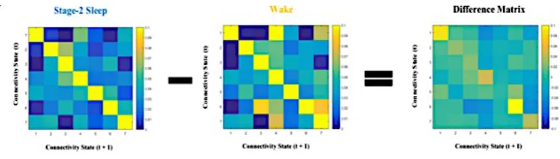
3.2.5 Transition Probabilities
Squares across the diagonal in each matrix (WAKE, STAGE-2 SLEEP) are marked by a
hotter color (yellow), indicating a high probability of staying in a particular state (Figure 11).
Cooler regions of the matrix, marked in blue, indicate the probability of switching between a
connectivity state on the y-axis into another state on the x-axis. A difference matrix was
computed by subtracting the probability matrix of Wake from the probability matrix of Stage-2
Sleep to highlight transition differences between conditions. Interestingly, the probability of
staying in connectivity state-1 and connectivity state-6 was greater in Stage-2 Sleep than in
Wake. This result complements aforementioned findings that show a higher frequency of
expression of connectivity state 1 and 6 in Stage-2 sleep. Furthermore, the probability of
transition from connectivity state-6 into 3 and from connectivity state-1 into 4 was higher in
Wake than in Stage-2 Sleep.
3.3 Heart Rate
Participants’ heart rate in Wake and Stage-2 Sleep did not significantly differ t(20) = 1.568, ns
(Figure12).
Figure 12. Mean heart rate (beats per minute) in Wake and Stage-2 Sleep. There was no difference in heart rate between conditions.
4.0
Discussion
4.1 Mean vs. Dynamic FC
Consistent with previous findings, there were no differences between stationary mean FC
across Wake and Stage-2 Sleep (Horovitz et al., 2008; Larson-Prior et al., 2009). In both
conditions, stationary mean FC matrices were marked by strong positive correlations within
functional networks, and weaker positive correlations and anti-correlations between functional
networks. These findings, although interesting, remain quite puzzling in light of evidence that
20 30 40 50 60 70
Wake Stage-2
shows a marked change in network connectivity between wakefulness and sleep. For instance,
the role of the canonical DMN has been shown as a potential mediator for conscious awareness
(Boly et al., 2009; Cauda et al., 2009; Sämann et al., 2011; Tagliazucchi, von Wegner, et al.,
2013). Coupling between anterior and posterior nodes of the DMN have been shown to
breakdown as individuals transition from wakefulness into deep sleep (Horovitz et al., 2009).
Examining spatial features of FC is important insofar as it explores changes in network
connectivity across different conscious states. However, as previously reported observations
suggests (Allen et al., 2017), mean FC does not fully characterize changes in FC; therefore,
temporal features of FC that may differentiate between wakefulness and sleep were explored.
Given that the conventional stationary approach obscures temporal features of FC, a
novel analytical method — dynamic FC (Allen et al., 2014) — was employed to reveal these
features. Using dynamic methods, evidence that supports the Slow Sleep Brain hypothesis was
found. By counting the number of transitions made between connectivity states, the brain was
markedly slower while asleep than awake. Not surprisingly, slower transitions between
connectivity states also impacted dwell time, as the analysis revealed longer mean dwell times
across states in sleep. These findings complement previous reports showing a breakdown in
effective connectivity during sleep (Massimini et al., 2005, 2010). A shift from globally
integrated brain networks to disintegrated local sub-networks reduction is expected to decrease
brain dynamics. Accordingly, the causal firing of neurons on the firing of other neuronal groups
would translate to an increase in the average dwell time across connectivity states.
Computational models of brain function during a loss of consciousness (under sedation)
show that coupling strengths between different nodes (i.e., brain regions) are weak, yet present
spatial features of functional connections, and underscore the importance of investigating
temporal features of FC (Deco et al., 2013). They highlight that temporal delays may impact the
location of coupling instability without impacting the actual spatial architecture of FC (Deco et
al., 2013). Given that stationary mean FC is an aggregate of all functional connections over time,
these short, transient, and weak connections may be misinterpreted as absent. Stationary mean
FC methods allow us to observe dominant spatial features of FC that were present in the data
over time; while dynamic FC methods allows us to examine recurrent patterns of FC over time
while also assessing temporal features of FC. Therefore, combining stationary and dynamic
methods offers a more comprehensive view of changes in spatial and temporal features of FC
across changes in conscious state, as well as, across different cognitive and behavioural states.
4.2 The
oretical Accounts
The slowing of the brain during sleep is instantiated in theoretical accounts that argue for
a critical point that the brain functions at during wakefulness — a point between ordered and
disordered dynamics (Petermann et al., 2009). At criticality, the brain’s functional activity is
governed by spatiotemporal and stochastic fluctuations that lead to multi-stable functional
connectivity states (Deco, Jirsa, & McIntosh, 2011; Deco et al., 2013; Dehaene & Changeux,
2005; Ghosh, Rho, McIntosh, Kötter, & Jirsa, 2008; Hudetz, Liu, & Pillay, 2015). It has been
hypothesized that these functional properties allow individuals to vigilantly attend to the external
environment and access cognitive resources as needed. Indeed, there has been evidence that
show support for this hypothesis by showing an association between temporal aspects of FC
associated with conscious and unconscious awareness (Kucyi & Davis, 2014). In contrast, while
in order and decrease in flexibility (Carhart-Harris et al., 2014). Furthermore, criticality during
wakefulness is analogous to goldilocks conditions, such that the brain is functioning at
equilibrium — not too fast and not too slow. Therefore, based on findings presented in this
thesis, it can be argued that the brain needs to dynamically and flexibly explore different
functional states while awake resulting in faster and more frequent transition between
connectivity states.
The criticality characterization of brain dynamics complements other theoretical work
that describes the relationship between cortical entropy and consciousness (Carhart-Harris et al.,
2014). Entropy is a measure of the degree of order in a system, such that a disordered state is
characterized with high entropy (Carhart-Harris et al., 2014). Accordingly, the brain can be
described as less entropic during sleep (i.e., increase order and more rigidness) as fewer
transitions and an increase in dwell time are observed. Changes in cortical entropy has also been
implicated in disorders of consciousness showing a decrease in entropy in unconscious states
(Gosseries, Schnakers, & Ledoux, 2011; Sleigh, Steyn-Ross, Steyn-Ross, Grant, & Ludbrook,
2004). Further, increases in cortical entropy have been observed in rats recovering from
anesthesia. An increase in cortical entropy in wakefulness is also characterized by an increases in
cortical information and transmission capacities, thus neural activity can be described as
scale-free (Fagerholm et al., 2016). This is complementary to work that have shown that FC during
wakefulness is scale-free when compared to sleep (Fagerholm et al., 2016; Lei, Wang, Yuan, &
Chen, 2014). These dynamic characterizations of the brain while awake are intuitive from the
standpoint of cognitive flexibility. A more entropic brain allows for more flexible and adaptive
The transition from wakefulness to sleep has also been examined using the Hurst
exponent (H), a measure of long-term memory of time series. A marked reduction in H (towards
values close to .5)has been observed during sleep compared to wakefulness indicating a
reduction in long-range memory in regional time series (Tagliazucchi, von Wegner, et al., 2013).
A value of H equal to .5 indicates a reduction in autocorrelation, and consequently, the potential
lack of temporal correlation. An H value between .5 and 1 indicates long-range positive
auto-correlations, which are interpreted as a system with increased long-range memory in regional
time series. In light of presented findings, these conclusions seem contradictory and
counter-intuitive given that temporal characteristics of FC slow down during sleep. An increase in H
during sleep would be predicated when compared to wakefulness given that the brain is cycling
less between different connectivity states, and dwelling for longer times in each state. These
temporal characteristics during sleep would indicate that there is an increase in long-range
memory in regional time series. However, the Hurst exponent is arguably not ideal in
characterizing brain dynamics and time-series auto-correlations because the Hurst exponent is
often used to examine stationary signals with a time-independent mean and variance. However,
the present findings show that BOLD fluctuations are time-dependent indicating that the signal is
non-stationary and thus the mean and/or the variance is not constant over time.
4.3 Connectivity States
The clustering approach adopted in this thesis revealed seven connectivity states that
represented recurrent connectivity patterns in wakefulness and Stage-2 Sleep. Interestingly, three
of the seven connectivity states had unique frequencies of expression. The selectivity of
al., 2015) and highlights that the transitions between different states may not be random, but due
to unique differences in spatial features of FC in wakefulness and sleep. Previous reports have
shown that FC patterns in awake macaques departs away from the brain’s structural connectivity;
comparatively, while under sedation, spatial features of FC markedly resemble the brain’s
structural connectivity (Barttfeld et al., 2015). A change in spatial features of FC is aligned with
a spatio-temporal hypothesis that posit a change in spatial and temporal features of FC (e.g.,
Bharat Biswal, Zerrin Yetkin, Haughton, & Hyde, 1995; Kannurpatti et al., 2008; Pillow et al.,
2008; Shmuel & Leopold, 2008). This hypothesis is grounded in the information integration
theory of consciousness (Tononi, 2004; Tononi et al., 2016), that argues that spatial and temporal
changes in FC mediate consciousness. Other empirical evidence that show support for
spatio-temporal changes in FC due to a change in arousal stem from animal studies that employ
invasive techniques such as optic and voltage imaging (Fagerholm et al., 2016; Fekete, Pitowsky,
Grinvald, & Omer, 2009). For instance, an increase in arousal in primates after undergoing
anesthesia is linked to an increase in the representational capacity of cortical space in the visual
cortex (Fekete et al., 2009). In other words, a change in the primates’ state of arousal had distinct
spatial and temporal functional features that overlapped the activity space (Fekete et al., 2009).
However, to definitively explore the uniqueness of the spatial features of the three
aforementioned connectivity states, a direct comparison of functional connectivity and structural
connectivity is needed as previously explored by Barttfeld et al. (2015).
The coupling relationships between functional networks, as observed in connectivity
state-1, resemble previously reported connectivity state that was described as hypersynchronous.
Cortical hypersynchrony describes the presence of strong coupling between all cortical networks
has been observed to be transient and short-lived (Hutchison et al., 2012). However, the
hypersynchronization of the cortex may be a result of functional integration to aid in cortical
synaptic plasticity (Acsády & Harris, 2017; Areal, Warby, & Mongrain, 2017) — a document
effect of sleep (Acsády & Harris, 2017; Diering et al., 2017). This view is aligned with
aforementioned findings given that connectivity state-1 was more frequently expressed and had a
higher mean dwell time in Stage-2 Sleep than in wakefulness. Cortical hypersynchrony has been
also been linked to brain plasticity in clinical settings observed in patients with Alzheimer’s
disease and with epilepsy (Noebels, 2011), and patients with head traumas (Santhakumar,
Ratzliff, Jeng, Toth, & Soltesz, 2001; Schiff, 2006), which has been linked to brain plasticity.
Therefore, temporal, and potential spatial, changes in FC may play a critical role in rewiring the
brain to allow for day-to-day experience to impact brain function and development. Together,
this line of evidence underscores the importance of revealing temporal changes in FC as they
have the potential to supplement existing clinical biomarkers that assess consciousness (Casali et
al., 2013; King et al., 2013; Sitt et al., 2014).
4.4
Limitations
4.4.1 Stationary Analysis
Stationary analysis revealed minimal qualitative differences between Wake and Stage-2
Sleep mean FC. A quantitative assessment using spatial correlation confirmed this qualitative
assessment. Upon a closer look, subtle differences were detected using a difference matrix. FDR
corrected (p < .01) t-tests performed on the difference matrix revealed five coupling relationships
between ICs that survived the correction (1 SC-VIS, 3 SM-VIS, and 1 CC-CB) (Figure 4). They
relationship between select functional families. The stationary analysis performed in this thesis
was compressive given that it considered whole-brain ICs. The significant differences revealed,
however, are hard to interpret in light of other research evidence that showed no differences
between Wake and Stage-2 Sleep in specific functional networks (e.g., DMN, Horovitz et al.,
2008), and whole-brain networks (Larson-Prior et al., 2009). Future research should examine
these relationships in more detail on a whole-brain levels, as well as, on specific network levels.
4.4.2 Dynamic Analysis
Mean dwell times of the four connectivity states discussed in this thesis are limited in
their interpretation given that the analysis was selective. An omnibus statistical test was
performed on the mean dwell times of four connectivity states that had significant frequency
differences in wake and sleep. The selectivity of this analysis remains open to criticism because
it would be expected to have differences in dwell times in states that had frequency differences in
Wake and Stage-2 Sleep. However, this choice was made to minimize the number of potential
pairwise comparisons made should the omnibus F-test was significant.
4.4.3 Statistical Criteria
Statistical testing on the Stationary Difference Matrix was conduction on 861
comparisons, while dynamic analyses were performed on a much smaller number of
comparisons (i.e., seven and four comparisons were conducted on connectivity state frequency
and dwell time, respectively). Therefore, the statistical criterion used for stationary mean FC is
arguable more stringent than the criterion used for dynamics analysis. For that reason,
Bonferroni corrections were performed on dynamic pairwise comparisons, while FDR