Volume 2006, Article ID 76278, Pages1–15 DOI 10.1155/ASP/2006/76278
Evaluating Edge Detection through Boundary Detection
Song Wang, Feng Ge, and Tiecheng Liu
Department of Computer Science and Engineering, University of South Carolina, Columbia, SC 29208, USA
Received 27 February 2005; Revised 6 June 2005; Accepted 30 June 2005
Edge detection has been widely used in computer vision and image processing. However, the performance evaluation of the edge-detection results is still a challenging problem. A major dilemma in edge-edge-detection evaluation is the difficulty to balance the objectivity and generality: a general-purpose edge-detection evaluation independent of specific applications is usually not well defined, while an evaluation on a specific application has weak generality. Aiming at addressing this dilemma, this paper presents new evaluation methodology and a framework in which edge detection is evaluated through boundary detection, that is, the likelihood of retrieving the full object boundaries from this edge-detection output. Such a likelihood, we believe, reflects the performance of edge detection in many applications since boundary detection is the direct and natural goal of edge detection. In this framework, we use the newly developed ratio-contour algorithm to group the detected edges into closed boundaries. We also collect a large data set (1030) of real images with unambiguous ground-truth boundaries for evaluation. Five edge detectors (Sobel, LoG, Canny, Rothwell, and Edison) are evaluated in this paper and we find that the current edge-detection performance still has scope for improvement by choosing appropriate detectors and detector parameters.
Copyright © 2006 Hindawi Publishing Corporation. All rights reserved.
1. INTRODUCTION
Edge detection is a very important feature-extraction meth-od that has been widely used in many computer vision and image processing applications. The basic idea of most avail-able edge detectors is to locate some local object-boundary information in an image by thresholding and skeletonizing the pixel-intensity variation map. Since the earliest work by Julez [1] in 1959, a huge number of edge detectors has been developed from different perspectives (e.g., [2–9]). A very natural and important question is then: which edge detec-tor and detecdetec-tor-parameter settings can produce better edge-detection results? This strongly motivates the development of a general and systematic way of evaluating the edge-detection results.
Prior edge-detection evaluation methods can be catego-rized in several ways. First, they can be classified as subjec-tive and objecsubjec-tive methods. The former uses the human-visual observation and decision to evaluate the performance of edge detection. Given the inherent inconsistency in hu-man perception, subjective evaluation results may exhibit a large variance for different observers. In objective meth-ods, quantitative measures are defined based solely on im-ages and the edge-detection results. Second, edge-detection evaluation methods can be categorized according to their re-quirement of the ground truth. With the ground truth, edge detection can be quantitatively evaluated in a more credible
way. Without the ground truth, some local coherence in-formation [10] is usually used to measure the performance. Third, edge-detection evaluation methods can be categorized based on test images: synthetic-image-based methods and real-image-based methods. A more detailed discussion on various edge detectors and edge-detection evaluation meth-ods can be found in [11].
Although many edge-detection evaluation methods have been developed in the past years (e.g., [11–15]), this is still a challenging and unsolved problem. The major challenge comes from the difficulty in choosing an appropriate per-formance measure of the edge-detection results. In most ap-plications, edge detection is used as a preprocessing step to extract some low-level boundary features, which are then fed into further processing steps, such as object finding and recognition. Therefore, the performance of edge detection is difficult to define without embedding it into certain applica-tions. However, if edge detection is evaluated based on the performance of a special application [13,16], such an evalu-ation may not be applicable to other applicevalu-ations. This intro-duces a well-known dilemma inherent in the edge-detection evaluation: general-purpose evaluation is difficult to define, while evaluation based on a specific application reduces the generality of the evaluation method.
(1) Generality: the evaluation measure should be well quantified yet generally applicable.
(2) Objective evaluation with ground truth: the evalua-tion measure should be objective to avoid potential incon-sistency in subjective evaluation. It should also use ground truth to achieve a credible evaluation.
(3) Real image: real (noisy) images should be used for evaluation, as prior research has revealed that conclusions drawn from synthetic images are usually not applicable to real images.
(4) Large data set: a convincing edge-detection evalua-tion should be conducted in a large set of real images and the results should be drawn through statistical analysis.
Considering these desirable features, we present in this paper a new method for edge-detection evaluation. The ma-jor novelty of this method is to evaluate edge detection in the framework of boundary detection, that is, detecting a full closed boundary of the salient object in an image. The basic idea is straightforward: although edge-detection results have been used for different applications, one of the fundamen-tal goals of edge detection in many applications is to detect some compact object-boundary information that can facil-itate further image processing. As shown inFigure 1, from the detected edges, we can estimate how likely it is that the complete geometry of the salient object boundaries present in this image will be determined. The likelihood of deter-mining the full object boundaries, to some extent, reflects the edge-detection performance on many applications, such as object recognition, tracking, and image retrieval, although those applications may notexplicitlyhave a component to de-rive full object boundaries out of the edge-detection results. Therefore, using this boundary-detection likelihood to eval-uate edge detection not only makes the problem well defined but also avoids overly sacrificing of the generality of the eval-uation.
To achieve this goal, we collect a set of real images each of which consists of an unambiguous foreground salient ob-ject and a noisy background. In these images, the ground-truth object boundary can be unambiguously extracted by manual processing, which enables an objective and quanti-tative measurement of the boundary-detection performance. A major component in our framework is to find a reliable algorithm for detecting a salient closed boundary from the edge-detection results. In this paper, we use our recently de-veloped ratio-contour algorithm to achieve this goal. In [17], we show the superiority of the ratio-contour algorithm over other existing algorithms for detecting salient closed bound-ary in a set of detected edges. In particular, this ratio-contour algorithm integrates the Gestalt laws of closure, continuity, and proximity, which are well-known properties to describe the perceptual saliency of an object boundary. In addition, it guarantees global optimality in boundary detection without requiring any kinds of initialization.
A related but simpler study was carried out by Baker and Nayar [12], where edge detection was evaluated us-ing some specified global coherence measures. In particular, they constructed a set of images in which the ground-truth boundaries were known to be a single straight line, two
Object recognition Tracking Image retrieval · · ·
Boundary detection
Edge detection
Figure 1: The likelihood of extracting full boundaries from de-tected edges reflects the performance of edge-detection algorithms in general applications.
parallel lines, two intersected lines, or an ellipse. In this way, the edge detection could be evaluated by checking these edges’ conformance to the four a priori known global co-herence measures. In this paper, the likelihood of locating a foreground object boundary can be treated as a more gen-eral global coherence measure, which is applicable to much wider classes of real images than the specified measures used in [12]. Furthermore, without constructing and applying the ground truth, Baker and Nayar’s method [12] requires that the test image contains no or very weak background noise. This substantially reduces its applicability and generality be-cause good edge detections should not only extract more salient-boundary features, but also suppress the background noise. The evaluation method proposed in this paper ad-dresses the problem effectively by testing algorithms on real noisy images and incorporating the ground-truth bound-aries.
In the remainder of this paper,Section 2gives a precise formulation of evaluating edge detection in terms of bound-ary detection. Section 3 discusses the detailed settings for each component of our edge-detection evaluation.Section 4 briefly describes the edge detectors used for evaluation in this paper. For this paper, we chose five edge detectors: Sobel [9], LoG [18], Canny [3], Rothwell [19], and Edison [20] for eval-uation.Section 5reports and analyzes the evaluation results on the collection of 1030 real images. A short conclusion, together with a brief discussion on future work, is given in Section 6.
2. EVALUATION FRAMEWORK
As mentioned above, our goal is to evaluate edge detection according to the likelihood of locating the ground-truth ob-ject boundary from edge-detection results. Therefore, we need first to have a boundary-detection algorithm that can locate a salient closed boundary from a set of detected edges. The coincidence between the detected boundary and the ground-truth object boundary is then used to measure the performance of the edge detection, as shown in Figure 2. Following many prior human-vision and computer-vision studies, we formulate the boundary detection as a
boundary-grouping process, in which a closed boundary is
Performance evaluation
Manual extraction Ground-truth boundary Difference measure Input
image
Edge detection Edge map Line approximation
Fragment map
Boundary grouping
Salient-object boundary
Figure2: An illustration of the framework for evaluating edge detection through boundary detection. The three components in the dashed-curve box comprise a boundary detection system.
Starting from a real image, this boundary-detection system consists of three sequential components: edge detection, line approximation, and boundary grouping, as shown in the dashed-line box inFigure 2.
In the first component, an edge detector, together with some specified detector parameters, is used to detect a set of edges, that is, sequences of connected edge pixels, from an input image. These edge pixels may result from the salient object boundary or background noise. Note that an 8-con-nected pixel neighborhood system is usually used to trace the connected edge pixels. In the second component, our goal is to derive the edge direction, that is, the boundary di-rection at each detected edge pixel, which plays an impor-tant role in measuring the boundary saliency and guiding the boundary grouping. The edges augmented with direc-tion informadirec-tion are calledfragmentsin this paper. In the last component, our goal is to identify a subset of the fragments and sequentially connect them into a closed boundary that is to be aligned with the most salient object in the input im-age. To achieve the boundary closure, we need to fill in the gaps between the neighboring fragments in this boundary connection.
There are several important problems that need to be ad-dressed in this framework to make this evaluation more con-vincing. First, it is particularly important to collect a large set of test images that are suitable for evaluation. On the one hand, the collected images should be real images with cer-tain variety and complexity. For example, they should con-tain various types and levels of noise. On the other hand, the ground-truth object boundary must be able to be manually extracted in an unambiguous way, that is, from the same im-age, different people should perceive the same salient object. This problem will be discussed in detail inSection 3.1.
Second, we need to choose a set of typical edge detec-tors and their typical detector parameters for evaluation. As the first component in this framework, different edge detec-tors or different detector parameters produce different edge maps on the same image. We then compare and evaluate these edge maps by comparing the accuracy of boundary de-tection in terms of the ground-truth boundary in this im-age. One consideration is that our selected edge detectors should cover both classical and recent ones. The selection of edge detectors and their parameters will be discussed in Section 4.
Third, we need to choose an appropriate algorithm to estimate and represent fragments, that is, edges with direc-tion informadirec-tion. Some edge detectors [3] have a nonmax-imum suppression step, which provides an estimation of the edge directions. However, the nonmaximum suppression step usually only considers a small neighborhood and the es-timated directions are very sensitive to the image noise, as ex-plained in detail in [19,20]. To address this problem and also make this edge-direction estimation component consistent in all edge detectors, we adopt a line-approximation algo-rithm to fit the edges by some line segments, providing more accurate and robust edge direction estimation. This way, each fragment is in the form of a straight line segment, as shown inFigure 2. We will discuss this in detail inSection 3.2.
Finally, we need to choose a quantitative criterion for measuring the coincidence between the detected boundary and the ground-truth boundary. Such a criterion should be insensitive to possible small errors introduced in the manual construction of the ground truth. We will discuss this prob-lem inSection 3.4.
3. EVALUATION SETTINGS
3.1. Test-image database
We collected 1030 real natural images from the internet, dig-ital photos, and some well-known image databases such as Corel for the proposed edge-detection evaluation. We care-fully examined each image before including it into our test-image database. A particular requirement is that each im-age contains a single perceptually unambiguous foreground salient object and a noisy background. Figure 3 demon-strates several sample images in our test-image database. In these images, we extract the ground-truth object boundary by simple manual processing. Note that, with the percep-tual unambiguity in distinguishing the foreground object and background noise, we can assume that the ground-truth boundary is unique for each image and is largely in-dependent on the specific person who manually extract this truth boundary. Samples of the extracted ground-truth boundaries are also shown inFigure 3. We intention-ally collect images with various foreground objects, such as human, animal, vehicle, building, and so forth. To facilitate the evaluation, all the images are unified to 256-bit gray-scale images in PGM format, with a size in the range of 80×80 to 200×200.
Note that our real-image database has completely differ-ent use to the real-image database in the Berkeley bench-mark [21], where the goal is to evaluate various region-based image-segmentation algorithms. In the Berkeley benchmark, an image may contain many complex structures and there-fore, the manual segmentation of the same image may be quite different across different people. If we use the Berkeley benchmark for our edge-detection evaluation, it would pose a much higher requirement for the boundary-grouping algo-rithm and greatly complicate the measure-criteria definition given that there is no unique ground truth. On the contrary, our carefully selected images have no such problems: the ground truth has no ambiguity and detecting a single salient boundary from the noisy background makes fewer demands on the boundary-grouping algorithm. We also believe that our collected images are sufficient, to a large extent, for the edge-detection evaluation because, in essence, edge detection is a local processing involving with the foreground structure and background noise, both of which have been included in all our collected images. However, our image database may not be suitable for general image-segmentation evaluation, because many natural images contain hierarchical structures that are not present in our collected images.
Our image database also differs from the real-image database used in the South Florida benchmark [11], where the goal is also for edge-detection evaluation. Because the South Florida benchmark evaluates edge detection using
Figure 3: Nine sample images in our image database and the ground-truth boundaries manually extracted from them.
a subjective method, the images used in its benchmark con-tain more complicated structures and there exists no single ground-truth boundary. As our main focus is edge-detection evaluation instead of studying human psycho-visual differ-ences in image understanding, we only select test images with unambiguous foreground and background, which in fact makes objective and quantitative evaluation possible. Differ-ent from the subjective evaluation method, objective evalua-tion methods can usually be extended to a large image data set. Therefore, our image database is much larger than the one used in the South Florida benchmark, which contains only 28 real images.
3.2. Line-approximation algorithm
differ in the mathematical formulations and the algorithmic solutions, the underlying basic ideas are the same: finding a set of line segments that are well aligned with the detected edges pixels. A key parameter in the line approximation is the dislocation-tolerance thresholdδt, which is the preassigned allowed discrepancy (in pixels) between an edge pixel and its mapping in the resulting line segments. With this parameter, the line-approximation method can find a minimum num-ber of line fragments to fit all the edges. In this paper, we use an implementation by Peter Kovesi for the line approxi-mation. This is a Matlab code that can be downloaded from http://www.csse.uwa.edu.au/∼pk/Research/MatlabFns/. Note that this implementation is not developed based on any special edge detectors.
To achieve an objective edge-detection evaluation, we need to consider the influence of selecting differentδt’s on the boundary-detection performance. Clearly, a smaller δt will generate more shorter line fragments and a largerδtwill generate fewer longer line fragments. InSection 5.1, we will conduct an empirical study on the influence ofδt. From this empirical study, we find that, regardless of the adopted edge-detectors and detector parameters, the sameδt always pro-vides us the best boundary-detection performance. There-fore, we can fix the parameterδt(and the line-approximation component) in the edge-detection evaluation.
3.3. Ratio-contour algorithm
In this paper, we use the ratio-contour algorithm [17] to im-plement the boundary-grouping component. In this algo-rithm, boundary saliency is measured by an unbiased com-bination of three important Gestalt laws:closure,proximity,
andcontinuity, which have been verified by many previous
psychological and psychophysical studies. Specifically,closure
requires the boundary to be complete.Proximityrequires the gap between two neighboring fragments to be small.
Con-tinuity requires the resulting boundary to be smooth. The
ratio-contour algorithm always detects the global optimal boundary in terms of its boundary-saliency measure.
To achieve closed boundaries, we construct a set of smooth curve segments, as shown by the dashed curves in Figure 4(b), to connect the constructed fragments. Those dashed curves are another set of fragments. To distinguish them from the initial straight-line fragments, we call them
virtual fragments and call the initial ones real fragments.
Considering the boundary smoothness, the virtual fragments are constructed in such a way that each of them interpolates two real-fragment endpoints inG1-continuity, that is, con-tinuous locations and concon-tinuous tangent directions [22], as shown inFigure 4(c). Various gap-filling algorithms can be used for constructing the smooth virtual fragments, and in this paper, we use the Bezier-curve splines to construct them. Ideally, we need to construct virtual fragments between each possible pair of fragment endpoints, as shown in Figure 4(c). In practice, however, we only construct virtual fragments that are likely to be along a salient closed bound-ary, as shown inFigure 4(b). A detailed discussion on this can be found in [17]. Based on the constructed real/virtual
fragments, a valid closed boundary can be defined as a cycle that traverses a subset of real fragments and virtual frag-ments alternately, as shown inFigure 4(d). The goal of the boundary grouping is then to find from all such valid closed boundaries the one that has the largest perceptual saliency. Letv(t) = (x(t),y(t)),t ∈ [0,L(v)], be the arc-length pa-rameterized representation [23] of a valid closed boundary, that is,v(L(v))=v(0), whereL(v) is the boundary length. In the ratio-contour algorithm [17], thecost(negatively related to thesaliency) of this boundary is defined by
R(v)=
L(v) 0
σ(t) +λ·κ2(t)dt
L(v) , (1)
whereσ(t)=1 ifv(t) is on a gap-filling virtual fragment and
σ(t)=0, otherwise.κ(t) is the curvature of the boundary at v(t).
In the numerator of (1), the first term0L(v)σ(t)dtmakes it biased towards a boundary with longer real fragments and shorter virtual fragments. This reflects the preference for bet-ter proximity. The second bet-term0L(v)κ2(t)dtreflects the favor of smoother boundaries, or better continuity. The denom-inator normalizes the cost by the boundary lengthL(v) to avoid a bias to shorter boundaries. λ > 0 is a regulariza-tion factor that balances the proximity and continuity in the cost function. Boundary closure is included as the hard con-straint in this algorithm: it only searches for closed bound-aries. In [17], a graph-theoretic algorithm is developed to find the optimal closed boundary that globally minimizes the cost (1). We can see that the ratio-contour algorithm well in-tegrates the properties of proximity, continuity, and closure into boundary grouping.
Several facts make the ratio-contour algorithm an appro-priate choice for the boundary-grouping component in our evaluation framework. First, boundary grouping itself is a very challenging problem and so far, only a few algorithms can achieve closed boundaries from fragments. A compar-ison study in [17] has shown that the ratio-contour algo-rithm usually has a better performance than the prior state-of-art boundary-grouping methods. Second, both the-oretical and experimental study in [17] has shown that the ratio-contour algorithm is able to detect the salient closed boundary from noisy background if the edge-detection step extract sufficient boundary features. Particularly, in [17], the ratio-contour algorithm was tested on a large set of synthetic data that mix the fragments from the sampled ground-truth boundary and noise and a very high boundary-detection accuracy was reported. Finally, the ratio-contour algorithm finds the globally optimal boundary in terms of its boundary-saliency measure and does not require any subjec-tive or heuristic initialization. This preserves the objectivity of our edge-detection evaluation framework.
3.4. Performance measure
Γ2
Γ1
Γ3
(a)
Γ2
Γ1
Γ3
(b)
Γ− 1
Γ+
1 Γ+2 Γ−
2
(c)
Γ2
Γ1
Γ3
(d)
Figure4: An illustration of the boundary grouping using the ratio-contour algorithm. (a) Straight-line fragments constructed from the edge-detection results. (b) Filling gaps between each pair of real-fragment endpoints withG1-continuity. (c) Between each pair of real
fragments, there are four possible gaps to fill without considering filling the gap between the two endpoints of the same real fragment. (d) The closed boundary extracted using the ratio-contour algorithm.
(a) (b) (c)
Figure5: An illustration of the region-based performance measure. (a) Original image; (b) the ground-truth boundary (dashed curve) and the detected boundary (solid curve); (c) the performance mea-sure|A∩B|/|A∪B|.
applications. The coincidence between the detected bound-ary and the ground-truth boundbound-ary reflects the performance of the adopted edge detection. If we measure the coincidence of these two boundaries in terms of two smooth curves, the resulting measure would be sensitive to the construction of the ground-truth boundary: even a small error there may in-troduce a larger error to the performance evaluation. In this paper, we adopt a region-based measure to accomplish this goal. Each image is a priori known to have a single salient closed boundary. Let region Arepresent the ground-truth salient object. We perform an edge detection (with certain edge detector and certain detector parameters) on this image and then use the ratio-contour algorithm to detect a salient closed boundary, which, in fact, generates a regionBfor the estimated salient foreground object. Denote the image asI, the edge detector as, and the detector parameters asμ. As illustrated inFigure 5, we measure the edge-detection
P(I,,μ)= |A∩B| |A∪B| =
|A∩B|
|A|+|B| − |A∩B|, (2) where| · |is the operation of computing the region area.
The numerator,|A∩B|, measures how much the true ob-ject region is detected. The denominator,|A∪B|, is a normal-ization factor which normalizes the performance measure to the range of [0, 1]. A performance of 1 is achieved if and only if the detected boundary completely coincides with the ground-truth boundary, that is,A = B. Zero performance indicates that there is no region-intersection between the
detected object and the ground-truth object. With this nor-malization factor, the performance measure penalizes mis-takenly detected regions (false positives). It is easy to see that this region-based measure is insensitive to small variations of the ground-truth boundary. This definition of the per-formance measure well incorporates the accuracy and recall measurement into one unified function, enabling quantita-tive, objecquantita-tive, and less computational intensive evaluation.
4. EDGE-DETECTORS SELECTED FOR EVALUATION
Considering both classical and recently-reported edge-de-tection methods, we chose five edge detectors: Sobel [9], LoG [18], Canny [3], Rothwell [19], and Edison [20] for evaluation. Each detector has its own parameter settings. In this paper, we evaluate not only different edge detectors, but also different parameter settings. Samples of edge-de-tection results using these five edge detectors are demonstrat-ed in Figure 6. In this paper, we use the image-process-ing toolbox functions in Matlab for the Sobel, LoG, and Canny edge detectors. The Rothwell edge detector source code was downloaded from the ftp site of the South Florida Computer Vision Group (ftp://figment.csee.usf.edu/ pub/Edge Comparison/source code/) and the Edison edge detector was downloaded from the author’s web page at http://www.caip.rutgers.edu/riul/research/code.html. In this section, we briefly describe these five edge detectors and their parameters.
4.1. Sobel edge detector
The Sobel edge detector [9] is one of the earliest edge detec-tion methods. For many applicadetec-tions, it is used as a standard gradient computation method to retrieve the image gradient and edges. More specifically, the Sobel edge detector contains two directional filters:
Gx=
⎡ ⎢ ⎣
−1 0 1 −2 0 2 −1 0 1
⎤ ⎥
⎦, Gy=
⎡ ⎢ ⎣
−1 −2 −1
0 0 0
1 2 1.
⎤ ⎥
⎦ . (3)
vertical directions, respectively. Combining these two image-gradient components, the image-gradient magnitude is derived as |∇I(x,y)| =(Gx∗I)2+ (Gy∗I)2, where∗stands for the signal-convolution operation. From gradient magnitude to edges, a thresholdδsis applied to find edge pixels. This in-troduces an intrinsic difficulty in Sobel edge detection (and also in many other edge detectors), that is, how to select the best threshold and how sensitive the threshold is in terms of overall performance. The Matlab implementation we used provides a default dynamic thresholdδs. In our evaluation, we test different thresholdsδs = psδsby varying the scaling factor psin the range of [0.5, 1.5], that is,psis the only pa-rameter in evaluating the Sobel detector.
4.2. LoG edge detector
As first introduced in [18], the LoG (Laplacian of Gaussian) edge detector is a well-known method that exploits the sec-ond derivatives of pixel intensity to locate edges. The defini-tion of a LoG filter actually is a combinadefini-tion of a Laplacian operator and a Gaussian filter:
∇2G σ=
∂2
∂x2+
∂2
∂y2
Gσ, (4)
where a 2D symmetric Gaussian smoothing filterGσ is de-fined by
Gσ(x,y)= 1 2πσ2exp
−
x2+y2 2σ2
. (5)
In this edge detector, edges are detected by combining the information of the image-gradient magnitude and the zero-crossing points in the second-derivative map. One threshold
δLis critical for LoG edge detector: only when the pixel (a) is a zero-crossing point in the second-derivative map, and (b) has a gradient magnitude large thanδL, do we select it as an edge pixel. Similar to Sobel, we treatδLas a scaled ver-sion of the default value provided in the LOG implementa-tion in Matlab, and vary the scaling factorpLin the range of [0.5, 2.5]. In another word,pLis the only detector parameter for LOG in our evaluation.
4.3. Canny edge detector
The Canny edge detector [3] is one of the most widely used edge detectors in computer-vision and image-processing community. In many applications, The Canny edge detector has been used as the standard image preprocessing tech-nique. The Canny edge detector was shown to be superior to Sobel detector by subjective visual evaluation in [11]. In this paper, we include the Canny edge detector to see whether it does have more favorable performance in an objective and general boundary-detection framework. Canny edge detec-tion consists of four steps: noise suppression, gradient com-putation, non-maximal suppression, and hysteresis. The first two steps are the same as the ones used in the Sobel edge de-tector. In the non-maximal suppression, edge pixel and edge
direction are estimated by checking and tracing the neigh-boring pixels around pixels with large gradient magnitude. In the hysteresis, a high thresholdδhighand a low threshold
δloware applied to remove spurious edges: it locates the first edge pixel by requiring its gradient magnitude to be larger than δhigh and then traces the following edge pixels by re-quiring the gradient magnitude to be larger thanδlow. The unique feature of the Canny edge detector is its hysteresis step with a two-threshold operation. Usually,δhighhelps remove false positives andδlowhelps improve the edge-location ac-curacy. In general, the Canny edge detector has a tendency to detect long edges, which usually improves its performance in subjective evaluations. Similar to Sobel and Canny, we set
δlow = pcδlow andδhigh = pcδhighin our evaluation, where
δlow andδhigh are the defaults provided in Matlab. There-fore, the scaling factor pc is the only detector parameter and we also vary it in the range of [0.5, 2.5] in our evalua-tion.
4.4. Rothwell edge detector
Many edge detectors, including the Canny edge detector, per-form poorly at edge junctions and corners. As explained in [24], this is mainly caused by the difficulty in estimating the correct direction information at edge junctions and cor-ners. Consequently, edge detection usually produces incor-rect or incomplete topology around corners and junctions. The Rothwell edge detector [19] can partially address this problem in maintaining the scene topology of images. Sim-ilar to the Canny edge detector, the Rothwell edge detector applies Gaussian smoothing first to reduce image noise and then computes the gradient magnitude and direction. Unlike the Canny edge detector, the Rothwell edge detector only uses the low thresholdδlowin hysteresis to filter spurious edges, while using another image-dependent dynamic threshold to further reduce the number of detected edges. With this dy-namic threshold, it can detect edges with varied gradient magnitudes. It is indicated in [19] that the Rothwell edge detector has two advantages over other methods: subpixel accuracy of the detected edges and better performance at edge junctions. By choosing this detector into our evalua-tion, we expect to find whether these two advantages actually benefit the application of salient boundary detection. Since the Rothwell edge detector chooses its high threshold auto-matically, the only parameter in our evaluation is pr which controls the lower threshold δlow. We vary pr in the range of [3, 18], as suggested in the Rothewell implementation we used.
4.5. Edison edge detector
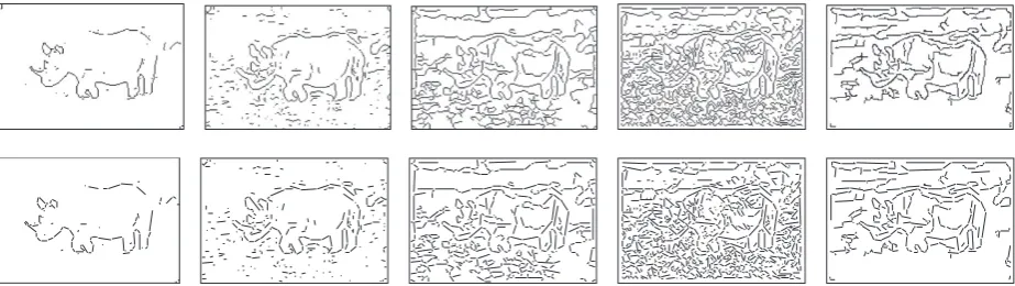
Figure6: Sample edge-detection and line approximation results. The original image is the first one shown inFigure 3. Top row shows edge-detection results from the five edge detectors with their default parameters. From left to right are the results from Sobel, LoG, Canny, Rothwell, and Edison, respectively. The bottom row shows the line-approximation results from the respective edge detection. SeeTable 1for the default parameters of each edge detector.
derive the edge confidence η, which measures the correla-tion between the considered edge and an ideal edge template with the same gradient direction. The gradient-magnitude confidenceρis calculated by counting the percentage of pix-els that have a gradient magnitude less than that of the con-sidered edge. Both confidence measures take values in the range of [0, 1]. In general, the Edison edge detector uses an approach similar to Canny to locate edge pixels and the ma-jor difference lies in that the Edison edge detector incorpo-rates these two confidence measures in the hysteresis step. In the Edison edge detector, two decision planes f(L)(η,ρ) andf(H)(η,ρ), which are determined by the confidence mea-suresηandρ, are calculated to replace the two fixed thresh-olds in Canny detector. In [20], it is claimed that these two decision planes introduce more flexibility and robustness to the edge detection. The Edison edge detector contains the maximum number (9 in total) of free parameters among all edge detectors. Obviously, it is neither possible nor necessary to exhaustively evaluate all of them. In our evaluation, we use the “boxed” decision planes and evaluate two most im-portant parameters, pH
e andpLe, where peH = ηhigh = ρhigh andpL
e =ηlow =ρlow. These two parameters determine the thresholds of confidence measures in the decision planes and we varied them in the range of [0.6, 1] in our evaluation.
5. PERFORMANCE EVALUATION
5.1. Line-approximation parameter selection
As discussed inSection 3.2, line approximation is the mid-dle step in our evaluation framework. Therefore we need to carefully select the line-approximation settings in or-der to compare edge detectors fairly. As mentioned in Section 3.2, the line-approximation algorithm has an impor-tant dislocation-tolerance parameterδtwhich gives the max-imal distance allowed for one edge pixel to be included in an approximated line segment. A smallδtgenerates many short fragments while a large one may produce long fragments that are not very well aligned with edge pixels.
First, we conducted experiments to show the sensitiv-ity of δt to boundary detection. The results are shown in Figure 7, which, together with all the other performance figures in Section 5, shows cumulative-performance his-togram curve, which describe the performance distribution on all 1030 images. As shown inFigure 7, thex-axis repre-sents the percentage of images, and the y-axis indicates the performance defined inSection 3.4. A data point (x,y) along a curve indicates that, under this specified setting, 100·x
percent of the images produce boundaries with an accuracy lower than y in terms of the given ground-truth bound-aries. Equivalently, this also means that 100·(1−x) per-cent of the images produce boundaries with performance better than y. Any change in the setting of edge-detection, line-approximation, or boundary-grouping components will produce a new performance curve for that setting. Obviously, the setting αachieves better performance than the setting
β if the performance curve ofα is above that of βin the cumulative-performance figure.
We variedδtin the line approximation for the five differ-ent edge detectors and some results are shown inFigure 7. This experiment was also conducted for many other detect-or-parameter settings, and just like the examples shown in Figure 7, all these experiments show thatδt = 1 almost al-ways produces the best performance for all the five detectors. Thus we conclude that this optimal value is largely uncorre-lated to the edge detectors and the detector parameters. For our evaluation, we simply chooseδt =1 in line approxima-tion for all of the remaining experiments.
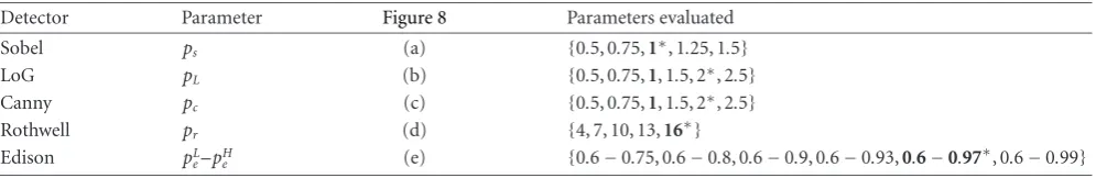
Table1: A summary of the edge detectors and their detector parameters that are evaluated inFigure 8. The numbers with “∗” are the best-average-performance parameters, and the numbers in bold face are the default parameters used in the implementations. Since Rothwell and Edison softwares provide no default parameters, we use their best-average-performance parameters as default ones.
Detector Parameter Figure 8 Parameters evaluated
Sobel ps (a) {0.5, 0.75,1∗, 1.25, 1.5}
LoG pL (b) {0.5, 0.75,1, 1.5, 2∗, 2.5}
Canny pc (c) {0.5, 0.75,1, 1.5, 2∗, 2.5}
Rothwell pr (d) {4, 7, 10, 13,16∗}
Edison pL
e–peH (e) {0.6−0.75, 0.6−0.8, 0.6−0.9, 0.6−0.93,0.6−0.97∗, 0.6−0.99}
large discrepancy from the ground truth boundary, which, consequently, seriously reduces the boundary detection per-formance.
5.2. Edge-detector performance
In this subsection, we conducted experiments to evaluate the performance of the five edge detectors described inSection 4. First, we evaluated each edge detector under different param-eter settings to investigate its sensitivity and optimality in terms of the detector parameters. The tested parameter set-tings for each detector are summarized in Table 1and the cumulative-performance histogram curves of each detector under various parameter settings are shown inFigure 8. The performance inFigure 8is derived from the experiments on all the images in our database.
In Figure 8, we also show an “optimal”-performance curve for each edge detector (the curve with the symbol “∗”). This represents the performance of each detector if we can dynamically find and apply the optimal parameter setting for each image.1More specifically, let
i represent theith edge detector, andμi j represent the jth parameter setting ofi. The performance ofion thenth imageInwith parameter
μi jis thenP(In,i,μi j), as defined in (2). The “optimal” per-formance of edge detectorion the imageInis defined as
Poptimal
In,i
=max
j
PIn,i,μi j
. (6)
The optimal-performance curve inFigure 8, to some extent, gives an upper-bound of the potential performance of an edge detector by varying parameters for each image.
Certainly, finding the optimal detector parameters for each image is usually a difficult problem. One easier way is to use a constant detector parameter for each detector. The question is which parameter can lead to best perfor-mance on all images. In this paper, we define the
best-average-performance (BAP) parametersto model such best constant
parameters. More specifically, for detectoriwith parameter
1Strictly speaking, the “optimal” is only defined in terms of parameter
spaces given inTable 1.
μi j, theaverage performanceon allNimages is
Pi,μi j
= 1
N
n
PIn,i,μi j
, (7)
and the BAP parameter isμi j∗with
j∗=arg maxjPi,μi j
. (8)
Obviously, for any imageInin the database,P(In,i,μi j∗)≤
Poptimal(In,i). The numbers inTable 1with the symbol “∗” indicate the BAP parameters for the five selected detectors.
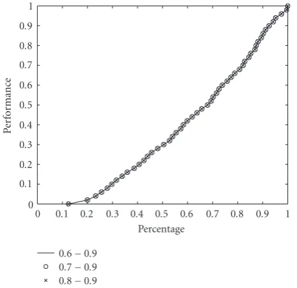
The Edison edge detector has two parameters,pL
eandpHe , which may substantially increase its parameter space in our evaluation. However, we find that when pH
e is fixed, peLhas little effect on performance, as shown inFigure 9. Therefore, we only vary parameterpH
e for Edison detector in the evalu-ation and the result is shown inFigure 8(e).
FromFigure 8, we have the following observations. First, detector-parameter selection has a large impact on the final performance. In fact, for all five edge detectors, varying the selected parameters usually results in significantly different boundary-detection performance. Second, the default edge-detector parameters in Matlab may not be optimal in terms of the proposed evaluation framework. For example, the per-formance of Canny detector is significantly improved by set-tingpc=2, that is, increasing the default thresholds by a fac-tor of 2. Third, for all five selected detecfac-tors, the performance with a fixed parameter is far below the optimal performance. This indicates that there is a considerable scope for perfor-mance improvement by dynamic parameter selection, that is, finding the optimal parameter for each individual image.
Table2: The number of winning images of each detector with different performance constraints.
Performance constraint Sobel LoG Canny Rothwell Edison Total no. of images
>0 230 184 213 219 184 1030
>0.35 189 145 177 180 161 852
>0.55 140 108 128 131 129 636
>0.75 70 45 73 70 77 335
>0.90 24 9 27 33 40 133
when the winning performance is larger than 0.75. From Table 2, we can see that Sobel, Canny, and Rothwell have a similar performance, while LoG does not perform quite as well. However, the difference is not significant among these five detectors. Particularly, for the images in which the boundary-detection accuracy is high (e.g., the row with the performance-constraint “>0.75”), Edison performs as well as Sobel, Canny, and Rothwell.
5.3. Combination of edge detectors
Beside evaluating and comparing the performance of indi-vidual edge detectors, it is also important to know whether and how these edge detectors are statistically related. If these five detectors can complement each other in edge detec-tion, then it would be worthwhile to investigate ways to boost the performance by combining them. To better under-stand the correlation of these five edge detectors, we intro-duce a virtualcombined detector, in which the winning edge detector for each image is used to process this image. We name the performance of such a virtual detector ascombined
performance:
Pcombined
In,µ
=max
i
PIn,i,μi
. (9)
Note that in the combined detector, the parameters for each individual detector are fixed and preset, and are denoted byμi for detectori, and in (9),µ= {μi,i=1, 2,. . ., 5}is the set consisting of the five fixed parameters. This combined per-formance gives the upper-bound perper-formance by switching edge detectors (with fixed detector parameters) on each im-age.
Figure 10 shows the performance of all five detectors (with BAP parameters), their respective optimal perfor-mance, and the combined performance using the BAP pa-rameters (labelled as “combined”). Again, we first see that these five edge detectors have similar performance with their BAP parameters. This is consistent with the information pro-vided inTable 2. In addition,Figure 10shows an interesting result: switching edge detectors with BAP parameters for individual images can drastically improve the final perfor-mance, and the combined performance of these five edge de-tectors is even slightly better than the optimal performance of each individual edge detector. This clearly indicates that these five edge detectors can complement each other to get much better performance.
Figure 11 compares the combined performance when each detector uses its BAP parameter and the combined performance when each detector uses its default parame-ter. The result shows very close performance between them. Combining the results shown inFigure 10, we see that, even using only default parameters for each detector, we may still achieve highly improved edge-detection performance if we have a way to select a suitable detector for each image.
InFigure 10, we also show a curve of the “ideal” per-formance. This performance is obtained by finding the best possible performance through edge-detector switching and detector-parameter optimization for each individual image; that is,
Pideal
In
=max
i,j
PIn,i,μi j
. (10)
We can see that the ideal performance is much higher than the performance of each individual edge detector. This tells us that, without developing new edge detectors, if we can find suitable detector and detector parameters for each image, we can get much better performance than that provided by any current individual detector.
In Figure 10, we can find that, even using a detector with the ideal performance, there is still a significant portion (20%–40%) of images with low performance. This may be a result of the boundary-grouping component. It is a rec-ognized fact that boundary grouping is a very challenging problem and a perfect boundary detection for any image is almost impossible. Yet this does not diminish the significance of our work since our main goal is to evaluate edge detection rather than boundary grouping. To further justify our evalu-ation results, we apply a performance constraint to exclude the low-performance images which are less discriminating in differentiating edge detector performance. This data selec-tion is based on one assumpselec-tion: if the boundary detecselec-tion fails with all possible edge detectors and detector parameters, we can hardly judge which edge detector is better. But if some fail and some succeed, we can incorporate such data for com-parison.
1 0.9 0.8 0.7 0.6 0.5 0.4 0.3 0.2 0.1 0
Pe
rf
o
rm
an
ce
0 0.1 0.2 0.3 0.4 0.5 0.6 0.7 0.8 0.9 1 Percentage
0.5 1 2
3 4 (a) Sobel
1 0.9 0.8 0.7 0.6 0.5 0.4 0.3 0.2 0.1 0
Pe
rf
o
rm
an
ce
0 0.1 0.2 0.3 0.4 0.5 0.6 0.7 0.8 0.9 1 Percentage
0.5 1 2
3 4 (b) LoG
1 0.9 0.8 0.7 0.6 0.5 0.4 0.3 0.2 0.1 0
Pe
rf
o
rm
an
ce
0 0.1 0.2 0.3 0.4 0.5 0.6 0.7 0.8 0.9 1 Percentage
0.5 1 2
3 4 (c) Canny
1 0.9 0.8 0.7 0.6 0.5 0.4 0.3 0.2 0.1 0
Pe
rf
o
rm
an
ce
0 0.1 0.2 0.3 0.4 0.5 0.6 0.7 0.8 0.9 1 Percentage
0.5 1 2
3 4 (d) Rothwell
1 0.9 0.8 0.7 0.6 0.5 0.4 0.3 0.2 0.1 0
Pe
rf
o
rm
an
ce
0 0.1 0.2 0.3 0.4 0.5 0.6 0.7 0.8 0.9 1 Percentage
0.5 1 2
3 4 (e) Edison
Optimal 1
0.9 0.8 0.7 0.6 0.5 0.4 0.3 0.2 0.1 0
Pe
rf
o
rm
an
ce
0 0.1 0.2 0.3 0.4 0.5 0.6 0.7 0.8 0.9 1 Percentage
0.5 0.75 1
1.25 1.5 (a) Sobel
Optimal 1
0.9 0.8 0.7 0.6 0.5 0.4 0.3 0.2 0.1 0
Pe
rf
o
rm
an
ce
0 0.1 0.2 0.3 0.4 0.5 0.6 0.7 0.8 0.9 1 Percentage
0.5 0.75 1
1.5 2 2.5 (b) LoG
Optimal 1
0.9 0.8 0.7 0.6 0.5 0.4 0.3 0.2 0.1 0
Pe
rf
o
rm
an
ce
0 0.1 0.2 0.3 0.4 0.5 0.6 0.7 0.8 0.9 1 Percentage
0.5 0.75 1
1.5 2 2.5 (c) Canny
Optimal 1
0.9 0.8 0.7 0.6 0.5 0.4 0.3 0.2 0.1 0
Pe
rf
o
rm
an
ce
0 0.1 0.2 0.3 0.4 0.5 0.6 0.7 0.8 0.9 1 Percentage
4 7 10
13 16 (d) Rothwell
Optimal 1
0.9 0.8 0.7 0.6 0.5 0.4 0.3 0.2 0.1 0
Pe
rf
o
rm
an
ce
0 0.1 0.2 0.3 0.4 0.5 0.6 0.7 0.8 0.9 1 Percentage
0.6−0.75 0.6−0.8 0.6−0.9
0.6−0.93 0.6−0.97 0.6−0.99 (e) Edison
1 0.9 0.8 0.7 0.6 0.5 0.4 0.3 0.2 0.1 0
Pe
rf
o
rm
an
ce
0 0.1 0.2 0.3 0.4 0.5 0.6 0.7 0.8 0.9 1 Percentage
0.6−0.9 0.7−0.9 0.8−0.9
Figure9: Performance evaluation on Edison detector by varying parameterpL
e. Result indicates thatpLehas little effect on the perfor-mance.
1 0.9 0.8 0.7 0.6 0.5 0.4 0.3 0.2 0.1 0
Pe
rf
o
rm
an
ce
0 0.1 0.2 0.3 0.4 0.5 0.6 0.7 0.8 0.9 1 Percentage
Ideal Combined Sobel-optimal LoG-optimal Canny-optimal Rothwell-optimal
Edison-optimal Sobel-BAP LoG-BAP Canny-BAP Rothwell-BAP Edison-BAP
Figure 10: Edge-detection evaluation on all 1030 images in the database.
Figure 10. All the conclusions drawn fromFigure 10can also be drawn fromFigure 12.
To summarize, we can draw the following conclusions from our performance-evaluation results.
(1) Line approximation is largely uncorrelated to the se-lected edge detectors in our evaluation framework. The line-approximation threshold can be selected within a certain
1 0.9 0.8 0.7 0.6 0.5 0.4 0.3 0.2 0.1 0
Pe
rf
o
rm
an
ce
0 0.1 0.2 0.3 0.4 0.5 0.6 0.7 0.8 0.9 1 Percentage
Combined-BAP Combined-default
Figure11: Comparison of the combined performance using default parameters (“combined-default”) and that using BAP parameters (“combined-BAP”).
range. Sub-pixel accuracy of edge detection is neither re-quired nor necessary for salient boundary detection.
(2) The overall performance of the five edge detectors is very similar. The performance difference is marginal and there is no obvious winner on the collected images.
(3) The selection of the detector parameters has signifi-cant impact on the final performance. The default parame-ters used in Matlab are not optimal for some edge detectors in terms of boundary-detection performance.
(4) The evaluated edge detectors do complement each other. With the right way of combining them, the perfor-mance can be greatly improved.
(5) Even without introducing new edge detectors, there is still considerable scope for performance improvement by optimizing parameters and/or by selecting the edge detector according to the input image.
6. CONCLUSION
1 0.9 0.8 0.7 0.6 0.5 0.4 0.3 0.2 0.1 0
Pe
rf
o
rm
an
ce
0 0.1 0.2 0.3 0.4 0.5 0.6 0.7 0.8 0.9 1 Percentage
Ideal Combined Sobel-optimal LoG-optimal Canny-optimal Rothwell-optimal
Edison-optimal Sobel-BAP LoG-BAP Canny-BAP Rothwell-BAP Edison-BAP
Figure12: Edge-detection evaluation on the selected 526 images with the ideal performance larger than 0.7.
The performance evaluation results show that the per-formance of these edge detectors is very similar but the de-fault parameters in these edge detectors are far from the best for boundary detection. There is considerable scope for per-formance improvement by introducing better dynamic pa-rameter selection. We also found that these edge detectors complement each other and an appropriate combination of them may improve the boundary-detection performance significantly. These findings naturally lead to two possi-ble future research directions: improving image-dependent detector-parameter selection and boosting performance with a combination of edge detectors.
ACKNOWLEDGMENTS
We would like to thank the anonymous reviewers for their in-sightful suggestions. This work was funded, in part, by NSF-EIA-0312861 and a grant from the University of South Car-olina Research and Productivity Scholarship Fund.
REFERENCES
[1] B. Julesz, “A method of coding TV signals based on edge de-tection,”Bell System Technology, vol. 38, no. 4, pp. 1001–1020, 1959.
[2] K. W. Bowyer, C. Kranenburg, and S. Dougherty, “Edge detec-tor evaluation using empirical ROC curves,”Computer Vision and Image Understanding, vol. 84, no. 1, pp. 77–103, 2001. [3] J. Canny, “A computational approach to edge detection,”
IEEE Transactions on Pattern Analysis and Machine Intelligence, vol. 8, no. 6, pp. 679–698, 1986.
[4] L. A. Iverson and S. W. Zucker, “Logical/linear operators for image curves,”IEEE Transactions on Pattern Analysis and Ma-chine Intelligence, vol. 17, no. 10, pp. 982–996, 1995.
[5] S. Konishi, A. L. Yuille, J. M. Coughlan, and S. C. Zhu, “Sta-tistical edge detection: learning and evaluating edge cues,” IEEE Transactions on Pattern Analysis and Machine Intelligence, vol. 25, no. 1, pp. 57–74, 2003.
[6] J. M. S. Prewitt, “Object enhancement and extraction,” in Pic-ture Processing and Psychopictorics, B. S. Lipkin and A. Rosen-feld, Eds., pp. 75–149, Academic Press, New York, NY, USA, 1970.
[7] K. R. Rao and J. Ben-Arie, “Optimal edge detection using expansion matching and restoration,” IEEE Transactions on Pattern Analysis and Machine Intelligence, vol. 16, no. 12, pp. 1169–1182, 1994.
[8] L. G. Roberts, “Machine perception of three-dimensional solids,” inOptical and Electro-Optical Information Processing, J. T. Tippett, Ed., pp. 159–197, MIT Press, Cambridge, Mass, USA, 1965.
[9] I. E. Sobel, “Camera models and machine perception,” Ph.D. dissertation, Stanford University, Stanford, Calif, USA, 1970. [10] L. Kitchen and A. Rosenfeld, “Edge evaluation using local edge
coherence,”IEEE Transactions on Systems, Man, and Cybernet-ics, vol. 11, no. 9, pp. 597–605, 1981.
[11] M. D. Heath, S. Sarkar, T. Sanocki, and K. W. Bowyer, “A robust visual method for assessing the relative performance of edge-detection algorithms,”IEEE Transactions on Pattern Analysis and Machine Intelligence, vol. 19, no. 12, pp. 1338– 1359, 1997.
[12] S. Baker and S. K. Nayar, “Global measures of coherence for edge detector evaluation,” inProceedings of IEEE Computer So-ciety Conference on Computer Vision and Pattern Recognition (CVPR ’99), vol. 2, pp. 373–379, Fort Collins, Colo, USA, June 1999.
[13] P. L. Palmer, H. Dabis, and J. Kitler, “A performance measure for boundary detection algorithms,”Computer Vision and Im-age Understanding, vol. 63, no. 3, pp. 476–494, 1996.
[14] Y. Yitzhaky and E. Peli, “A method for objective edge detec-tion evaluadetec-tion and detector parameter selecdetec-tion,”IEEE Trans-actions on Pattern Analysis and Machine Intelligence, vol. 25, no. 8, pp. 1027–1033, 2003.
[15] Q. Zhu, “Efficient evaluations of edge connectivity and width uniformity,”Image and Vision Computing, vol. 14, no. 1, pp. 21–34, 1996.
[16] X. Y. Jiang, A. Hoover, G. Jean-Baptiste, D. Goldgof, K. W. Bowyer, and H. Bunke, “A methodology for evaluating edge detection techniques for range images,” inProceedings of 2nd Asian Conference on Computer Vision (ACCV ’95), vol. 2, pp. 415–419, Singapore, December 1995.
[17] S. Wang, T. Kubota, J. M. Siskind, and J. Wang, “Salient closed boundary extraction with ratio contour,”IEEE Transactions on Pattern Analysis and Machine Intelligence, vol. 27, no. 4, pp. 546–561, 2005.
[18] D. Marr and E. C. Hildreth, “A theory of edge detection,” Proceedings of the Royal Society of London. Series B, vol. 207, no. 1167, pp. 187–217, 1980.
[19] C. A. Rothwell, J. L. Mundy, W. Hoffman, and V.-D. Nguyen, “Driving vision by topology,” inProceedings of IEEE Interna-tional Symposium on Computer Vision (ISCV ’95), pp. 395– 400, Coral Gables, Fla, USA, November 1995.
[20] P. Meer and B. Georgescu, “Edge detection with embedded confidence,”IEEE Transactions on Pattern Analysis and Ma-chine Intelligence, vol. 23, no. 12, pp. 1351–1365, 2001. [21] D. Martin, C. Fowlkes, D. Tal, and J. Malik, “A database of
Computer Vision (ICCV ’01), vol. 2, pp. 416–423, Vancouver, BC, Canada, July 2001.
[22] J. D. Foley, A. van Dam, S. K. Feiner, and J. F. Hughes, Com-puter Graphics: Principles and Practice in C, Addison Wesley, Reading, Mass, USA, 2nd edition, 1995.
[23] R. H. Bartels, J. C. Beatty, and B. A. Barsky,An Introduction to Splines for Use in Computer Graphics and Geometric Modelling, Morgan Kaufmann, Los Altos, Calif, USA, 1987.
[24] D. A. Forsyth and J. Ponce,Computer Vision: A Modern Ap-proach, Prentice-Hall, Upper Saddle River, NJ, USA, 2003.
Song Wang received his Ph.D. degree in electrical and computer engineering from the University of Illinois at Urbana-Cham-paign in 2002. From 1998 to 2002, he also worked as a Research Assistant in the Im-age Formation and Processing Group of the Beckman Institute, University of Illinois at Urbana-Champaign. Since August 2002, he has been an Assistant Professor in the De-partment of Computer Science and
Engi-neering at the University of South Carolina. His research interests include computer vision, medical image processing, and machine learning.
Feng Gereceived his B.S. degree from Ts-inghua University, Beijing, in July 2002. Since August 2004, he has been a Master student in the Department of Computer Science and Engineering at the University of South Carolina. His research interests are computer vision and medical imaging.
Tiecheng Liureceived the M.S. degree in electrical engineering from Chinese Acade-my of Sciences in 1999 and Ph.D. degree in computer science from Columbia Univer-sity in 2003. Since 2003, he was with the Department of Computer Science and En-gineering at the University of South Car-olina, where he is now an Assistant Pro-fessor. His main research interests include computer vision, image and video