Domain-Driven Classification Based on Multiple Criteria and Multiple Constraint-Level Programming for Intelligent Credit Scoring

(1)

For Peer Review Only

Domain Driven Classification based on Multiple

Criteria and Multiple Constraint-level

Programming for Intelligent Credit Scoring

Jing He,Yanchun Zhang, Yong Shi,

Senior Member, IEEE

, Guangyan Huang,

Member, IEEE

Abstract—Extracting knowledge from the transaction records and the personal data of credit card holders has great profit potential for the banking industry. The challenge is to detect/predict bankrupts and to keep and recruit the profitable customers. However, grouping and targeting credit card customers by traditional data-driven mining often does not directly meet the needs of the banking industry, because data-driven mining automatically generates classification outputs that are imprecise, meaningless and beyond users’ control. In this paper, we provide a novel domain-driven classification method that takes advantage of multiple criteria and multiple constraint-level programming for intelligent credit scoring. The method involves credit scoring to produce a set of customers’ scores that allows the classification results actionable and controllable by human interaction during the scoring process. Domain knowledge and experts’ experience parameters are built into the criteria and constraint functions of mathematical programming and the human and machine conversation is employed to generate an efficient and precise solution. Experiments based on various datasets validated the effectiveness and efficiency of the proposed methods.

Index Terms—Credit Scoring, Domain Driven Classification, Mathematical Programming, Multiple Criteria and Multiple Constraint-level Programming, Fuzzy Programming, Satisfying Solution

F

1 I

NTRODUCTION

Due to widespread adoption of electronic funds transfer at point of sale (EFTPOS), internet banking and the near-ubiquitous use of credit cards, banks are able to collect abundant information about card holders’ trans-actions [1]. Extracting effective knowledge from these transaction records and personal data from credit card holder holds enormous profit potential for the banking industry. In particular, it is essential to classify credit card customers precisely in order to provide effective services while avoiding losses due to bankruptcy from users’ debt. For example, even a 0.01% increase in early detection of bad accounts can save millions.

Credit scoring is often used to analyze a sample of past customers to differentiate present and future bankrupt and credit customers. Credit scoring can be formally defined as a mathematical model for the quantitative measurement of credit. Credit scoring is a straight-forward approach for practitioners. Customers’ credit behaviors are modeled by a set of attributes/variables. If

• J. He is with School of Engineering and Science, Victoria University, Australia and Research Center on Fictitious Economy and Data Science, Chinese Academy of Sciences, China. E-mail: [email protected]

• Y. Zhang is with School of Engineering and Science, Victoria University, Australia. E-mail:[email protected]

• Y. Shi is with the Research Center on Fictitious Economy and Data Science, Chinese Academy of Sciences, China and College of Information Science and Technology, University of Nebraska at Omaha, USA. E-mail: [email protected]

• G. Huang is with School of Engineering and Science, Victoria University, Australia. E-mail:[email protected]

a weight is allocated to each attribute, then a sum score for each customer can be generated by timing attribute values with their weights; scores are ranked and the bankrupt customers can be distinguished. Therefore, the key point is to build an accurate attribute weight set from the historical sample and so that the credit scores of customers can be used to predict their future credit behavior. To measure the precision of the credit scoring method, we compare the predicted results with the real behavior of bankrupts by several metrics (introduced later).

Achieving accurate credit scoring is a challenge due to a lack of domain knowledge of banking business. Previous work used linear and logistic regression for credit scoring; we argue that regression cannot provide mathematically meaningful scores and may generate results beyond the user’s control. Also, traditional credit analysis, such as decision tree analysis [4] [5], rule-based classification [6][7], Bayesian classifiers [8], near-est neighbor approaches [9], pattern recognition [10], abnormal detection [11][12], optimization [13], hybrid approach [14], neural networks [15] [16] and Support Vector Machine (SVM) [17] [18], are not suitable since they are data-driven mining that cannot directly meet the needs of users [2] [3]. The limitation of the data driven mining approaches is that it is difficult to adjust the rules and parameters during the credit scoring process to meet the users’ requirements. For example, unified domain related rules and parameters may be set before the classification commences, but it cannot be controlled since data driven mining often runs automatically.

(2)

For Peer Review Only

Our vision is that human interactions can be used to guide more efficient and precise scoring according to the domain knowledge of the banking industry. Linear Programming (LP) is a useful tool for discriminating analysis of a problem given appropriate groups (eg. ”Good” and ”Bad”). In particular, it enables users to play an active part in the modeling and encourages them to participate in the selection of both discriminate criteria and cutoffs (boundaries) as well as the relative penalties for misclassification [19] [20] [21].

We provide a novel domain-driven classification method that takes advantage of multiple criteria and multiple constraint-level programming (MC2) for intel-ligent credit scoring. In particular, we build the domain knowledge as well as parameters derived from experts’ experience into criteria and constraint functions of linear programming, and employ the human and machine conversation to help produce accurate credit scores from the original banking transaction data, and thus make the final mining results simple, meaningful and easily-controlled by users. Experiments on benchmark datasets, real-life datasets and massive datasets validated the effectiveness and efficiency of the proposed method.

Although many popular approaches in the banking industry and government are score-based [22], such as the Behavior Score developed by Fair Isaac Corporation (FICO) in [23], the Credit Bureau Score (also devel-oped by FICO) and the First Data Resource (FDR)’s Proprietary Bankruptcy Score [24], to the best of our knowledge, no previous research has explored domain-driven credit scoring for the production of actionable knowledge for the banking industry. The two major advantages of our domain-driven score-based approach are:

(1) Simple and meaningful. It outperforms traditional data-driven mining because the practitioners do not like black box approach for classification and prediction. For example, after being given the linear/nonlinear param-eters for each attribute, the staff of credit card providers are able to understand the meanings of attributes and make sure that all the important characteristics remain in the scoring model to satisfy their needs.

(2) Measurable and actionable. Credit card providers value sensitivity- the ability to measure the true positive rate (that is, the proportion of bankruptcy accounts that are correctly identified- the formal definition will be given later) but not accuracy [25]. Sensitivity is more important than other metrics. For example: a bank’s profit on ten credit card users in one year may be only

10∗ $ 100 = $ 1000 while the loss from one consumer

in one day may be $ 5000. So the aim of a two-class

classification method is to separate the ”bankruptcy” accounts (”Bad”) from the ”non-bankruptcy” accounts (”Good”) and to identify as many bankruptcy accounts as possible. This is also known as the method of ”making black list” [26]. This idea decides not only the design way for the classification model but also how to measure the model. However, classic classification methods such as

SVM [17] [18], decision tree [27] and neural network [15] that pay more attention to gaining high overall accuracy but not sensitivity cannot satisfy the goal.

Using LP to satisfy the goal of achieving higher sen-sitivity, the problem is modeled as follows.

In linear discriminate models, the misclassification of data separation can be expressed by two kinds of objectives. One is to minimize the internal distance by minimizing the sum of the deviations (MSD) of the observations from the critical value and the other is to maximize the external distance by maximizing the minimal distances (MMD) of observations from the crit-ical value. Both MSD and MMD can be constructed as linear programming. The compromise solution in Multiple Criteria Linear Programming (MCLP) locates the best trade-off between linear forms of MMD and MSD as data separation.

In the classification procedure, although the boundary

of two classes, b (cutoff), is the unrestricted variable

in model MSD, MMD and MCLP, it can be pre-set by the analyst according to the structure of a particular

database. First, choosing a proper value ofbas a starting

point can speed up solving the above three models.

Second, given a threshold τ, the best data separation

can be selected from results determined by different b

values. Therefore, the parameter b plays a key role in

achieving the desired accuracy and most mathematical

programming based classification models use b as an

important control parameter [19], [29], [30], [21], [22], [26], [28],[22], [39].

Selection of the b candidate is time consuming but

important because it will affect the results significantly. Mathematical programming based classification calls for

a flexible method to find a better cutoff b to improve

the precision of classification for real-time datasets. For this reason, we convert the selection process of cutoff as the multiple constraints and construct it into the programming model. With the tradeoff between MSD and MMD, the linear programming has been evolved as multiple criteria and multiple constraint-level linear programming. The potential solution in MC2 locates the best trade-off between MMD and MSD with a better cutoff in a given interval instead of a scalar.

However, this trade-off cannot be guaranteed to lead to the best data separation even if the trade-off provides the better solution. For instance, one method with a high accuracy rate may fail to predict a bankruptcy. The decision on the ”best” classification depends powerfully on the preference of the human decision makers. The main research problem addressed by this paper is to seek an alternative method with trade off of MMD and MSD, cutoff constraint and human cooperation for the best possible data separation result: we shall refer to it as the domain driven MC2-based classification method. Thus, following the idea of L. Cao, C. Zhang and etc. [2] [3], the core of our novel MC2-based method is as follows: we model domain knowledge into criteria and constraint function for programming. Then, by

(3)

For Peer Review Only

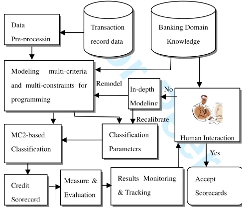
ment and evaluation, we attain feedback for in-depth modeling. In this step, human interaction is adopted for choosing suitable classification parameters as well as re-modeling after monitoring and tracking the process, and also for determining whether the users accept the scoring model. This human machine conversation process will be employed in the classification process. A framework of domain-driven credit scoring and decision making process is shown in Fig. 1.

Data Pre-processin

Modeling multi-criteria and multi-constraints for programming

MC2-based Classification Credit Scorecard

Classification Parameters Measure &

Evaluation

Results Monitoring & Tracking

Accept Scorecards Transaction

record data

Banking Domain Knowledge

Yes Human Interaction In-depth

Modeling No Remodel

Recalibrate

Fig. 1. Domain Driven Credit Scoring and Decision

Making Process

An advantage of our domain-driven MC2-based method is that it allows addition of criterion and con-straint functions to indicate human intervention. In particular, the multiple criteria for measuring the de-viation and the multiple constraints to automatically select the cutoff with a heuristic process to find the user’s satisfied solution will be explored to improve the classification model. Another advantage of our MC2 model is that it can be adjusted manually to achieve a better solution, because the score may be not consistent with the user’s determination. Instead of overriding the scoreboard directly, the credit manager can redefine the objectives/constraints/upper boundary and the interval

of cutoffb to verify and validate the model.

Therefore, in this paper, our first contribution is to provide a flexible process using sensitivity analysis and interval programming according to domain knowledge of banking to find a better cutoff for the general LP based classification problem. To efficiently reflect the human intervention, we combine the two criteria to measure the deviation into one with the interval cutoff and find the users’ satisfying solution instead of optimal solution. The heuristic process of MC2 is easily controlled by the banking practitioners. Moveover, the time-consuming process of choosing and testing the cutoff is changed to a automatic checking process. The user only needs to input

an interval and the MC2 linear programming can find a

best cutoffb for improving precision of classification.

To evaluate precision, there are four popular measure-ment metrics: accuracy, specificity, sensitivity and K-S (Kolmogorov-Smirnov) value, which will also be used to measure the precision of credit scoring throughout this paper, given as follows. Firstly, we define four concepts. TP (True Positive): The number of Bad records classified correctly. FP ( False Positive): The number of Normal records classified as Bad. TN(True Nega-tive): The number of Normal records classified cor-rectly. FN (False Negative): The number of Bad records classified as Normal. In the whole paper, ”Normal”

equals to ”Good”. Then, Accuracy = T N+T P

T P+F P+F N+T N, Specif icity = _{F P}T N₊_{T N},Sensitivity = _{T P}T P₊_{F N}. Another metric, the two-sample KS value, is used to measure how far apart the distribution functions of the scores of the ”good” and ”bad” are: the higher values of the metrics, the better the classification methods. Thus, another contribution of this paper is that through ex-ample and experiments based on various datasets, we analyze the above four metrics as well as the time and space complexity to prove the proposed algorithm outperforms three counterparts: support vector machine (SVM), decision tree and neural network methods.

The rest of this paper is organized as follows: Section 2 introduces an LP approach to credit scoring based on previous work. Section 3 presents details of our domain-driven classification algorithm based on MC2 for achieving intelligent credit scoring. In Section 4, we evaluate the performance of our proposed algorithm by experiments with various datasets. Our conclusion is provided in Section 5.

2 L

INEAR

P

ROGRAMMING

A

PPROACH 2.1 Basic Concepts of LP

A basic framework of two-class problems can be

pre-sented as follows: GivenAiX ≤b,A∈B and AiX ≥b,

A ∈ G, where r is a set of variables (attributes) for a

data seta= (a1, ..., ar), Ai= (Ai1, ..., Air) is the sample

of data for the variables,i= 1, ..., nandnis the sample

size, the aim is to determine the best coefficients of the

variables, denoted byX = (x1, ..., xr)T, and a boundary

(cutoff) valueb(a scalar) to separate two classes: G and B.

For credit practice,Bmeans a group of ”bad” customers,

Gmeans a group of ”good” customers.

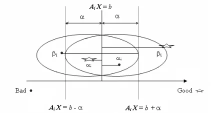
In our previous work [22][26], to accurately measure the separation of G and B, we defined four parameters for the criteria and constraints as follows:

αi: the overlapping of two-class boundary for caseAi

(external measurement);

α: the maximum overlapping of two-class boundary

for all casesAi (αi< α);

βi: the distance of caseAi from its adjusted boundary

(internal measurement);

β: the minimum distance for all cases Ai from its

adjusted boundary (βi > β).

(4)

For Peer Review Only

To achieve the separation, the minimal distances of ob-servations from the critical value are maximized (MMD). The second separates the observations by Minimizing the Sum of the Deviations (MSD) of the observations. This deviation is also called “overlapping”. A simple version of Freed and Glover’s [19] model which seeks MSD can be written as:

(M1) Min Σiαi,

s.t. AiX ≤b+αi, Ai∈B (1)

AiX > b−αi, Ai∈G

where Ai,b are given,X is unrestricted andαi≥0.

The alternative of the above model is to find MMD:

(M2) Max Σiβi,

s.t. AiX≥b−βi, Ai∈B (2)

AiX < b+βi, Ai ∈G

where Ai,b are given,X is unrestricted andβi≥0.

A graphical representation of these models in terms of

α and β is shown in Fig. 2. We note that the key point

of the two-class linear classification model is to use a linear combination of the minimization of the sum of

αi or maximization of the sum of βi. The advantage of

this conversion is that it allows easy utilization of all techniques of LP for separation, while the disadvantage is that it may miss the scenario of trade-offs between these two separation criteria [26].

Fig. 2. Overlapping Case in Two-class Separation of LP Model.

A hybrid model (M3) in the format of multiple criteria linear programming (MC) that combines models of (M1) and (M2) is given by [26][22]:

(M3) Minimize Σiαi,

Maximize Σiβi,

AiX=b+αi−βi, Ai∈B,

AiX=b−αi+βi, Ai∈G

(3)

where Ai, b are given, X is unrestricted, αi ≥ 0 and

βi≥0.

Y

Database, M1 Model & A Given Threshold W

Select b0pairs

¦

i Min D

Choose best as Xa*_{, b}

0*

ExceedsW

N

Stop

Sensitivity analysis for b0*

Mark as checked and select another pairs

Fig. 3. A Flowchart of Choosing the b candidate for M1.

2.2 Finding the cutoff for Linear Programming 2.2.1 Sensitive analysis

Instead of finding the suitable b randomly, this paper

puts forward a sensitivity analysis based approach to

find and test b for (M1) shown in Fig. 3. Cutoff b for

(M2) can be easily extended in a straightforward way.

First, we select b0 and −b0, as the original pair for

the boundary. After (M1), we choose a better value, b∗

0,

between them. In order to avoid duplicate checking for

some intervals, we find the changing interval4b∗ _for_b∗

to keep the same optimal solution by sensitivity analysis [31]. (Users can see the detailed algorithm and proof in Appendix 1).

In order to reduce computation complexity, when we continue to check the next cutoff for (M1), it is better

to avoid b∗ ₊ ₄_b∗ _{interval. We label the interval as}

checked and the optimal solution for b∗ _{as the best}

classification parameters in the latest iteration. Similarly,

we can get the interval for −b∗ _{and it is obvious that}

if the optimal solution is not the better classification

parameters, −b∗ ₊₄₍₋_b)∗ _{is labelled as checked, too.}

After another iteration, we can gain the different optimal

results for anotherXa∗0

from another pair. Note that the

nextXa∗0

may not be better thanXa∗_{; if it is worse, we}

just keep Xa∗ _{as the original one and choose another}

pair forb in the next iteration.

Basically, the sensitivity analysis can be viewed as a data separation through the process of selecting the

better b. However, it is hard to be sure whether the

optimal solution always results in the best data sepa-ration. Therefore, the main research problem in credit scoring analysis is to seek a method for producing higher

(5)

For Peer Review Only

Database, M1 Model & A Given Threshold W

M (3-1)

ExceedsW

M (3-2)

ExceedsW

N N

Stop

Y

Select [bL, bU]

Fig. 4. Interval Programming to Choose better b*.

prediction accuracy (like sensitivity for testing ongoing customers). Such methods may provide a near-optimal result, but lead a better data separation result. That is why we use a Man-Machine Interaction as shown in Fig. 3; this is a typical Human Cooperated Mining in domain driven process.

2.2.2 Interval programming

Using the interval coefficients for the right hand side

vector b in MSD and MMD can serve the purpose of

finding a better cutoff for the classification problem. Interval coefficients include not only interval numbers

but alsoα-cuts, fuzzy numbers [32]. The general solution

for interval linear programming can be found in [33]. We

assume that the entries of the right hand side vector b

are not fixed, they can be any value within prescribed

intervals: bil ≤ b ≤ biu, then the interval MSD (IMSD)

can be stated as:

(M3-1) Min Σiαi,

s.t. AiX ≤[bl, bu] +αi, Ai∈B (4)

AiX >[bl, bu]−αi, Ai∈G

where Ai,bl,bu are given,X is unrestricted andαi≥0.

The interval MMD (IMMD) can be stated as:

(M3-2) Max Σiβi,

s.t. AiX ≥[bl, bu]−βi, Ai∈B (5)

AiX <[bl, bu] +βi, Ai∈G

where Ai,bl,bu are given,X is unrestricted andαi≥0.

Similar to Fig.3, IMSD and IMMD process can be stated in Fig. 4 which can be adjusted dynamically to suit user preference.

3 P

ROPOSED

MC2 M

ETHODS

To improve the precision (defined by four metrics in Sec-tion 1) of the LP approach, we develop a new approach

in this paper. Firstly, we provide Domain Driven MC2-based (DDS-MC2) Classification, which models domain knowledge of banking into multiple criteria and multiple constraint-level programming. Then we develop Do-main Driven Fuzzy MC2-based (DDF-MC2) Classifica-tion, which is expected to improve the precision of DDS-MC2 further by adding human manual intervention into the credit scoring process and to reduce the computation complexity.

3.1 Domain Driven MC2 based Classification 3.1.1 MC2 Algorithm for Two-Classes Classification

Although sensitivity analysis or interval programming can be implemented into the process of finding a better cutoff for linear programming, it still has some inher-ent shortcomings. Theoretically speaking, classification models like (M1), (M2), (M3-1) and (M3-2) only reflect lo-cal properties, not global or entire space of changes. This paper proposes multiple criteria and multiple constraint-level programming to find the true meaning of the cutoff and an unrestricted variable.

A boundary valueb (cutoff) is often used to separate

two groups (recall (M1)), wherebis unrestricted. Efforts

to promote the accuracy rate have been confined largely

to the unrestricted characteristics of b. A given b is put

into calculation to find coefficients X according to the

user’s experience related to the real time data set. In such a procedure, the goal of finding the optimal solution for the classification question is replaced by the task of

testing boundaryb. Ifbis given, we can find a classifier

using an optimal solution. The fixed cutoff value causes another problem in that the probability of those cases that can achieve the ideal cutoff score would be zero. Formally, this means that the solutions obtained by linear programming are not invariant under linear transforma-tions of the data. An alternative approach to solve this

problem is to add a constant, ζ, to all the values, but

it will affect the weight results and performance of its classification, and unfortunately, it cannot be used for the method in [1]. Adding a gap between the two regions may overcome the above problem. However, if the score is falling into this gap, we must determine which class it should belong to [1].

To simplify the problem, we use a linear combination

of bλ _{to replace} _b _{to get the best classifier as} _X∗_(λ)_.

Suppose we now have the upper boundarybuand lower

boundary bl. Instead of finding the best boundary b

randomly, we find the best linear combination for the best classifier. That is, in addition to considering the criteria space that contains the tradeoffs of multiple criteria in (M1) and (M2), the structure of MC2 linear programming has a constraint-level space that shows all possible tradeoffs of resource availability levels (i.e. the

tradeoff of upper boundary bu and lower boundary of

bl). We can test the interval value for both bu and bl

by using a classic interpolation method such as those of Lagrange, Newton, Hermite, and Golden Section in real

(6)

For Peer Review Only

numbers [−∞,+∞]. It is not necessary to set negative

and positive values forblandbuseparately but it is better

to set the initial value ofblas the minimal value and the

initial value ofbuas the maximum value. So the internal

between [bl,bu] is narrowed down.

With the adjusting boundary, MSD (M1) and MMD (M2) can be changed from standard linear programming to linear programming with multiple constraints.

(M1-1) Min Σiαi,

s.t. AiX ≤λ1bl+λ2bu+αi, Ai∈B (6) AiX > λ1bl+λ2bu−αi, Ai∈G

λ1+λ2= 1 0≤λ1, λ2≤1

whereAi,bu,blare given,X is unrestricted andαi≥0.

(M2-1) Max Σiβi,

s.t. AiX≥λ1bl+λ2bu−βi, Ai∈B (7) AiX < λ1bl+λ2bu+βi, Ai∈G,

λ1+λ2= 1, 0≤λ1, λ2≤1

where Ai,bu,bl are given,X is unrestricted andβi≥0.

The above two programmings are LP with multiple constraints. This formulation of the problem always gives a nontrivial solution.

The combination of the above two models is with the objective space showing all tradeoffs of MSD and MMD:

(M4) Min Σiαi,

Max Σiβi,

s.t. AiX =λ1bl+λ2br+αi−βi, Ai∈B (8) AiX =λ1bl+λ2br−αi+βi, Ai∈G

λ1+λ2= 1, 0≤λ1, λ2≤1

where Ai, bu, bl are given, X is unrestricted, αi ≥ 0

and βi ≥0.

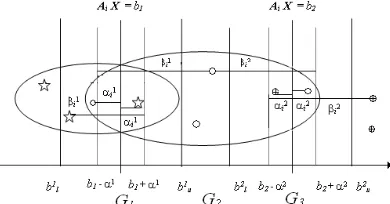
A graphical representation of MC2 models in terms of

αand β is shown in Fig. 5.

Fig. 5. Overlapping Case in Two-class Separation of MC2 model.

In (M4), theoretically, finding the ideal solution that simultaneously represents the maximal and the minimal

is almost impossible. However, the theory of MC linear programming allows us to study the tradeoffs of the criteria space. In this case, the criteria space is a two dimensional plane consisting of MSD and MMD. We use a compromised solution of multiple criteria and multiple constraint-level linear programming to minimize the

sum of αi and maximize the sum ofβi simultaneously.

Then the model can be rewritten as:

(M5) Max −γ1Σiαi+γ2Σiβi,

s.t. AiX =λ1bl+λ2br+αi−βi, Ai∈B (9) AiX=λ1bl+λ2br−αi+βi, Ai ∈G

γ1+γ2= 1 λ1+λ2= 1 0≤λ1, λ2≤1 0≤γ1, γ2≤1

where Ai, bu, bl is given, X is unrestricted, αi ≥ 0,

and βi ≥ 0, i = 1,2, ..., n. Separating the MSD and MMD, (M4) is simplified to LP problem with multiple constraints like (M3-1) and (M3-2). Replacing the

com-bination of bl and bu with the fixed b, (M4) becomes an

MC problem like (M3).

This formulation of the problem always gives a non-trivial solution and is invariant under linear

transforma-tion of the data.γ1 andγ2are the weight parameters for

MSD and MMD. λ1 and λ2 are the weight parameters

for bu and bl, respectively: they serve to normalize the

constraint-level and the criteria-level parameters. A series of theorems on the relationship among the solutions of LP, multiple criteria linear programming (MC) and MC2 are used to prove the correctness of the MC2-based classification algorithm. The detailed proof for the MC2 model can be found in Appendix 2.

3.1.2 Multi-class Classification

(M5) can be extended easily to solve a multi-class prob-lem (M6) shown in Fig. 6.

(M6) Max −γ1Σiαi+γ2Σiβi,

AiX=λ1bl+λ2bu+αi−βi,

Ai∈G1,

λ1k−1bkl−1+λk2−1buk−1−αki−1+βik−1=AiX =λk

1bkl +λk2buk−αki +βki,

Ai∈Gk, k= 2, ..., s−1

AiX=λs1−1bsl−1+λ2s−1bsu−1−αis−1+βis−1,

Ai∈Gs

λ1k−1bkl−1+λ2k−1bku−1+αik−1≤λk1bkl +λk2bku−αki, k= 2, ..., s−1, i= 1, ..., n

γ1+γ2= 1 (10) λ1+λ2= 1

0≤λ1, λ2≤1 (11)

whereAi,bku,bkl is given,Xis unrestricted,α

j

i ≥0, and

β_ij ≥0.

(7)

For Peer Review Only

Fig. 6. Three Groups Classified by Using MC2.

3.2 Domain-Driven Fuzzy MC2-based Classification

Instead of finding the ”optimal solution” (a goal value) for the MC2 model like M4, this paper aims for a ”sat-isfying solution” between upper and lower aspiration levels that can be represented by the upper and lower bounds of acceptability for objective payoffs. A fuzzy MC2 approach by seeking a fuzzy (satisfying) solution obtained from a fuzzy linear program is proposed as an alternative method to identify a compromise solution for MSD (M1-1) and MMD (M2-1) with multiple constraints. When Fuzzy MC2 programming is adopted to classify the ”good” and ”bad” customers, a fuzzy (satisfying) solution is used to meet a threshold for the accuracy rate of classifications, though the fuzzy solution is a near optimal solution for the best classifier. The advan-tage of this improvement of fuzzy MC2 includes two aspects: (1) reduced computation complexity. A fuzzy MC2 model can be calculated as linear programming. (2) efficient identification of the weak fuzzy potential solution/special fuzzy potential solution for a better separation. Appendix 3 show that the optimal solution

X∗ _{of M11 is a weak/special weak potential solution of}

(M4).

3.2.1 Fuzzy MC2

To solve the standard MC2 model like (M4), we use the idea of a fuzzy potential solution in [34] and [22]. Then the MC2 model can be converted into the linear format. We solve the following four (two maximum and two minimum) linear programming problems:

(M1-2) Min (Max) Σiαi,

s.t. AiX ≤λ1bl+λ2bu+αi, Ai∈B (12) AiX > λ1bl+λ2bu−αi, Ai∈G

λ1+λ2= 1 0≤λ1, λ2≤1

whereAi,bu,blare given,X is unrestricted andαi≥0.

(M2-2) Max (Min) Σiβi,

s.t. AiX≥λ1bl+λ2bu−βi, Ai∈B (13) AiX < λ1bl+λ2bu+βi, Ai∈G,

λ1+λ2= 1, 0≤λ1, λ2≤1

whereAi,bu,bl are given,X is unrestricted andβi ≥0.

Let u0

1 and l01 be the upper and lower bound for the

MSD criterion of (M1-2), respectively. Let u0

2 and l02 be

the upper and lower bound for the MDD criterion of

(M2-2), respectively. If x∗ _{can be obtained from solving}

the following problems (M11), then x∗ _∈ _X _{is a weak}

potential solution of (M11).

(M11) Maximize ξ,

ξ≤ Σαi−y1L

y1U−y1L,

ξ≤ Σβi−y2L

y2U −y2L,

AiX ≤λ1bl+λ2bu+αi, Ai∈B (14) AiX > λ1bl+λ2bu−αi, Ai∈G

AiX ≥λ1bl+λ2bu−βi, Ai∈B AiX < λ1bl+λ2bu+βi, Ai∈G, λ1+λ2= 1 0≤λ1, λ2≤1

where Ai, y1L, y1U, y2L, y2U, bl, bu are known, X is

unrestricted, andαi,βi,λ1,λ2,ξ≥0,i= 1,2, ..., n.

To find the solution for (M11), we can set a value ofδ,

and let λ1 ≥δ, λ2 ≥δ. The contents in Appendix 3 can

prove that the solution with this constraint is a special fuzzy potential solution for (M11). Therefore, seeking

M aximum ξ in the Fuzzy MC2 approach becomes the standard of determining the classifications between ”Good” and ”Bad” records in the database. Once model

(M11) has been trained to meet the given threshold τ,

the better classifier is identified.

(M11) can be solved as a linear programming and it exactly satisfies the goal of accurately identifying the ”good” and ”bad” customers. The proof of the fuzzy MC2 model can be found in Appendix 3.

3.2.2 Heuristic Classification Algorithm

To run the proposed algorithm below, we first create a data warehouse for credit card analysis. Then we gener-ate a set of relevant attributes from the data warehouse, transform the scales of the data warehouse into the same numerical measurement, determine the two classes of

”good” and ”bad” customers, classify thresholdτ that is

selected by the user, train and verify the set.

Algorithm:credit scoring by using MC2 in Fig. 7.

Input: the training samples represented by discrete-valued attributes, the set of candidate

at-tributes, interval of cutoffb, and a given

thresh-old by user.

Output: best b∗ _{and parameters X* for credit scoring.}

Method:

(3) Give a class boundary value bu _and _bl _and

use models (M1−1) to learn and computer the

overall scoresAiX(i= 1,2, ..., n) of the relevant

attributes or dimensions over all observations repeatedly.

(8)

For Peer Review Only

Sety₁U y1L N

N Y

Y

Y Database, MC2 Model & A Given Threshold W

Select buand bl

ExceedsW

ExceedsW M (2-1) M (1-1)

Sety _L y

2 2U

M (11)

ExceedsW

Stop

Fig. 7. A Flowchart of MC2 Classification Method.

(4) If (M1−1) exceeds the thresholdτ, go to (8), else

go to (5).

(5) If (M2−1) exceeds the thresholdτ, go to (8), else

go to (6).

(6) If (M11) exceeds the thresholdτ, go to (8), else

go to (3) to consider to give another cut off pair.

(7) Apply the final learned scoresX∗to predict the

unknown data in the verifying set.

(8) Find separation.

This approach uses MSD with multiple constraintsbas

(M1-1) as a tool for the first loop of classification. If the result is not satisfied, then it applies MMD with multiple

constraints b as (M2-1) for the second loop of

classifica-tion. If this also produces an unsatisfied result, it finally produces a fuzzy (satisfying) solution of a fuzzy linear program with multiple constraints, which is constructed from the solutions of MMD and MSD with the interval

cutoff, b, for the third loop of classification. The better

classifier is developed heuristically from the process of computing the above three categories of classification.

Note that for the purpose of credit scoring, a better classifier must have a higher sensitivity rate and KS value with acceptable accuracy rate. Given a threshold of correct classification as a simple criterion, the better classifier can be found through the training process once the sensitivity rate and KS value of the model exceeds the threshold. Suppose that a threshold is given, with

the chosen interval of cutoffb and credit data sets; this

domain driven process proposes a heuristic classification method by using the fuzzy MC2 programming (FLP) for intelligent credit scoring. This process has the char-acteristic in-depth mining, constraints mining, human cooperated mining and loop-closed mining in terms of domain driven data mining.

4 E

XAMPLE AND

E

XPERIMENTAL

R

ESULTS 4.1 An Example

To explain our model clearly, we use a data slice of the classical example in [19]. An applicant is to be classified as a ”poor” or ”fair” credit risk based on responses to two questions appearing on a standard credit applica-tion.

For the linear programming based model, users choose

the cutoffbrandomly. Ifbfalls into the scalar such as (-20,

-23), the user can generate an infinite solution set forX∗

such asX = (1,−4)t_{by the mathematical programming}

based model like (M1), (M2), (M1-1), (M1-2) and (M11).

Then the weighting schemeX∗_{will be produced to score}

the 4 customers, denoted by 4 points, and thus they can be appropriately classified by sub-dividing the scores

into intervals based on cutoffb∗shown in Tab. 1.

Suppose the scalar of b is set as [10,1000] by users;

then not all mathematical programming based model like (M2) and (M2-1) can produce the best classification model, and M11 shows its advantage.

TABLE 1

Credit Customer Data Set.

Responses Transformed

Scores Credit

Customer

Quest 1 (a1)

Quest 2

(a2) X=(1, -4)t Cutoff

1 3 4 -13

Group I

(Poor Risk) 2 4 6 -20

3 5 7 -23

Group II

(Fair Risk) 4 6 9 -30 b (-20,-23)

For (M11), we use a standard software package LINDO [37] to solve the following four linear program-ming problems instead of using MC2 software.

(M1-2’) Min (Max) α1+α2+α3+α4,

s.t. A1X < λ1bl+λ2bu+α1, A2X < λ1bl+λ2bu+α2, A3X ≥λ1bl+λ2bu−α3,

A4X ≥λ1bl+λ2bu−α4, (15) λ1+λ2= 1

0≤λ1, λ2≤1 1

(9)

For Peer Review Only

where Ai is given by Table 1, bl = 10, bu = 1000, X is

unrestricted and αi≥0.

(M2-2’) Max (Min) β1+β2+β3+β4,

s.t. A1X > λ1bl+λ2bu−β1, A2X > λ1bl+λ2bu−β2, A3X ≤λ1bl+λ2bu+β3,

A4X ≤λ1bl+λ2bu+β4, (16) λ1+λ2= 1

0≤λ1, λ2≤1

where Ai is given by Table 1, bl = 10, bu = 1000, X is

unrestricted and βi ≥0.

We obtain u0

1 is 0, l01 =−1000, u02 is unbounded and

set as 10000,l0

2= 3.33E−03. The we solve the following

fuzzy programming problem:

(M11’) Maximize ξ,

ξ≤α1+α2+α3+α4+ 1000

1000 ,

ξ≤ β1+β2+β3+β4−0.00333

10000−0.00333 , A1X < λ1bl+λ2bu+α1, A2X < λ1bl+λ2bu+α2, A3X ≥λ1bl+λ2bu−α3, A4X ≥λ1bl+λ2bu−α4, A1X > λ1bl+λ2bu−β1, A2X > λ1bl+λ2bu−β2, A3X ≤λ1bl+λ2bu+β3, A4X ≤λ1bl+λ2bu+β4, λ1+λ2= 1 0≤λ1, λ2≤1,

where Ai is given by Table 1, bl= 10,bu= 1000,X is

unrestricted, αi ≥0 and βi ≥0. The optimum solution

to the above (M11’) is X1 = 6.67 and X2 =−3.33. The

score for the four customers are 6.67, 6.67, 10 and 10

respectively. b∗ _{= 10}_{. This is a weak potential solution}

for the MC2 model like (M4). The two groups have been separated.

4.2 Experimental Evaluation

In this section, we evaluate the performance of our proposed classification methods using various datasets that represent the credit behaviors of people from dif-ferent countries, shown in Table 2, which includes one benchmark German dataset, two real-world datasets from the UK and US, and one massive dataset randomly generated by a public tool. All these datasets classify people as ”good” or ”bad” credit risks based on a set of attributes/variables.

The first dataset contains a German Credit card records from UCI Machine learning databases [38]. The set contains 1000 records (700 normal and 300 bad) and

Data Number Type

German datasets 1,000 Public data UK datasets 1,225 Real world data US datasets 5,000 Real world data NDC massive datasets 500,000 Generated by Public Tool

TABLE 2 Datasets

24 variables. The second is a UK bankruptcy dataset [1], which collects 307 bad and 918 normal customers with 14 variables. The third dataset is from a major US bank, which contains data for 5000 credit cards (815 bad and 4185 normal) [26][39] with 64 variables that describe cardholders’ behaviors. The fourth dataset includes 500,000 records (305,339 normal and 194,661 bad) with 32 variables is generated by a multivariate Normally Distributed Clustered program (NDC) [40].

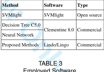
We also compare our proposed method with three classic methods: support vector machine (SVM light) [41], Decision Tree (C5.0 [27]) and Neural Network. All experiments were carried out on a windows XP P4 3GHZ cpu with 1.48 gigabyte of RAM. Table 3 shows the im-plementation software that was explored to run the four datasets. We implemented both LP methods (M1, M2) in Section 2 and the proposed DDF-MC2 methods (M1-1, M2-1 and Eq.M11) in Section 3 by using Lindo/Lingo [37] then used Clementine 8.0 to run both C5.0 and neural network algorithms, and at last compiled an open source SVM light in [41] to generate SVM results.

Method Software Type

SVMlight SVMlight Open source

Decision Tree C5.0

Neural Network

Clementine 8.0 Commercial

Proposed Methods Lindo/Lingo Commercial

TABLE 3 Employed Software.

We now briefly describe our experimental setup. Firstly, we studied both LP methods (M1 and M2) and the proposed DDF-MC2 methods (M1-1, M2-2 and M11) by analyzing real-world datasets and then chose the best one to compare with three counterparts: SVMlight, C5.0 and Neural Network. We validated our proposed best method in massive datasets to study scalability, as well as time efficiency and memory usage. All of the four methods - our proposed method and three counterparts - are evaluated by four metrics (e.g. accuracy, specificity, sensitivity and K-S value) that are defined in Section 1. We used Matlab [42] and SAS [43] to help compute K-S

(10)

For Peer Review Only

value. Our goal is to see if the best one of our methods performs better than the three counterparts, especially in terms of sensitivity and K-S value, without reducing accuracy and specificity.

4.2.1 Experimental Study of Proposed Methods

We chose real-world datasets from the US and UK to evaluate our proposed methods, because our methods are derived from a real world application project. From both Table 4 (US dataset) and Table 5 (UK dataset), overall, we can see that both the training values and test values of M11 exceed those of the other four methods in terms of sensitivity (except M1) and K-S value. As previously mentioned, these two metrics are the most important ones for helping users in the banking industry to make decisions. We also observe that the accuracy of M11 is slightly lower than for M1 and M1-2, but the specificity and K-S value of M11 are far better than those of M1 and M1-2. Therefore, M11 is the best method.

Accuracy Specificity Sensitivity KS Value Training 0.8435 0.0458 0.9989 11.07

M1

Test 0.8810 0.4768 0.9597 14.45

Training 0.6920 0.2841 0.7714 33.07

M2

Test 0.5239 0.1447 0.5978 33.03

Training 0.8387 0.079 0.9867 8.26

M1-2

Test 0.8261 0.0523 0.9768 4.25

Training 0.47 0.6413 0.4367 34.87

M2-2

Test 0.4283 0.6835 0.3786 34.31

Training 0.7625 0.8601 0.7435 62.34

M11

Test 0.7976 0.8034 0.7965 60.1

TABLE 4

10-fold cross-validation result of US dataset.

Accuracy Specificity Sensitivity KS Value Training 0.8985 0.3943 0.9967 40.1

M1

Test 0.8808 0.48 0.9589 44.89

Training 0.7277 0.42 0.7876 33.07

M2

Test 0.5579 0.3356 0.6012 33.03

Training 0.9054 0.483 0.9876 47.06

M1-1

Test 0.9001 0.4548 0.9868 45.67

Training 0.7619 0.8913 0.7367 62.87

M2-1

Test 0.704 0.8345 0.6786 51.31

Training 0.8306 0.921 0.813 73.44

M11

Test 0.819 0.8878 0.8056 69.35

TABLE 5

10-fold cross-validation result of UK dataset.

The MC2 method in this paper is the best for predict-ing ”Bad” accounts with a satisfied acceptable sensitivity rate of 0.7965 and the highest KS value (60.1). If the threshold on catching ”Bad” accounts is chosen based on a priciple in [2], then the MC2 method should be implemented to conduct the data-mining project. The MC2 method demonstrated its advantages over other mathematical programming methods like M1, M2, M1-1 and M2-M1-1 and is thus an alternative tool to the other well-known classification techniques.

4.2.2 Comparison to Three Counterparts

In this section, the best of our proposed methods, M11, is compared with three classic classification methods: SVMlight (SVM), Decision Tree (DT) and Neural Net-work (NN). In addition to two real world datasets (US and UK datasets), we adopt a public benchmark dataset (German dataset) to evaluate our method.

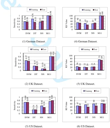
We can see from Fig. 8 (1-6), both the sensitivity and KS values of our method M11 excel those of SVMlight, Decision Tree and Neural Network in both training and test datasets of German, UK and US. Notably, the best sensitivity values of M11 for training and test benchmark datasets of German are nearly 1.0 and around 0.98 respectively, which almost double the values that are achieved by other three counterparts in Fig. 8 (1). The same trend is shown in Fig. 8 (4) that the best KS values of M11 are twice others’ values, nearly reaching 100. The sensitivity values of the SVM method rank second in all three datasets. The KS values of M11 are trible those of its counterparts in UK dataset. Also, in the US dataset, the KS values of M11 are slightly greater than for other three methods. In a summary, our method M11 outperforms other three methods in terms of sensitivity and KS value: it has better ability to distinguish ”bads”.

Fig. 8 shows various performances of M11 due to different datasets that have their own distinct properties reflecting the credit behavior of peoples from three coun-tries. These difference also ensure that the evaluation is objective. Overall, the common observation of the results based on three countries’ datasets is that the performance of M11 is always better than those of other three counterparts.

0

.5

8 0.7

6 0 .5 3 1 0 .5 6 0 .5

3 0.6 3 0 .9 8 0 0.2 0.4 0.6 0.8 1 S en si ti v it y

SVM DT NN M11 Training Test

(1) German Dataset.

5 0 4 5 4 3 1 0 0 4 8 3

4 48

1 0 0 0 20 40 60 80 100 K S V al u e

(4) German Dataset.

0 .5 7 0 .2 7 0 .1 0 0 .8 1 0 .5 5 0 .2 5 0 .1 0 0 .8 1 0 0.2 0.4 0.6 0.8 1 S en si ti v it y

(2) UK Dataset.

2

6

2

2 ₂3

7

3

2

0 24

6 9 0 20 40 60 80 100 K S V al u e

(5) UK Dataset.

0 .6 9 0 .2 4 0 .4 8 0 .7 4 0 .6 9 0 .2

4 0.3

8 0 .8 0 0 0.2 0.4 0.6 0.8 1 S en si ti v it y

(3) US Dataset.

4

7 55 60 62

4

5

4

1 48

6 0 0 20 40 60 80 100 K S V al u e

(6) US Dataset.

Fig. 8. Sensitivity and KS Value.

Although accuracy and specificity are not as important as sensitivity and K-S value in the banking industry, we also simply analyze them as follows. Overall, we can see from Fig. 9 (1-6) that the performance of M11 waves

(11)

For Peer Review Only

slightly above or below the other three methods in terms of both accuracy and sensitivity in three datasets. For example, the accuracy of M11 is slightly greater in the German and UK datasets and slightly lower in the US dataset than the other three methods. Also, the specificity of M11 is slightly greater in the German dataset and slightly less in the UK and US datasets than other three methods.

0

.6

6 0.90

0

.7

9 0.9

9 0 .6 4 0 .7 4 0 .7

8 0.9

8 0 0.2 0.4 0.6 0.8 1 A cc u ra cy

(1) German Dataset.

0

.8

4 0.9

6 0 .9 0 0 .9 8 0 .8 3 0 .8 4 0 .8

5 0.9

8 0 0.2 0.4 0.6 0.8 1 S p ec if ic it y

(4) German Dataset.

0

.6

0 0.7

7 0 .7 5 0 .8 3 0 .5

9 0.7

1 0 .7 0 0 .8 2 0 0.2 0.4 0.6 0.8 1 A cc u ra cy

(2) UK Dataset.

0 .6 1 0 .9 5 0 .9 8 0 .9 2 0 .6 0 0 .9

3 ₀.99

0 .8 9 0 0.2 0.4 0.6 0.8 1 S p ec if ic it y

(5) UK Dataset.

0 .7 3 0 .8 5 0 .8 5 0 .7 6 0 .7

3 0.8

7 0 .8 5 0 .8 0 0 0.2 0.4 0.6 0.8 1 A c c u ra c y

(3) US Dataset.

0

.7

4 0.9

7 0 .9 2 0 .8 6 0 .7

3 0.9

7 0 .9 2 0 .8 0 0 0.2 0.4 0.6 0.8 1 S p ec if ic it y

(6) US Dataset.

Fig. 9. Accuracy and Specificity.

4.2.3 Massive Data Evaluation

We used NDC in [40] to generate massive datasets as it is difficult to find massive data in real life. According to [48], we explain the NDC as follows: NDC firstly generates a series of random centres for multivariate normal distributions and then randomly generates a fraction of data for each centre. Also, NDC randomly generates a separating plane, based on which classes are chosen for each centre and then randomly generates the points from the distributions. NDC can increase inseparability by increasing variances of distributions. Since the separating plane is generated randomly, we may not control directly the degree of linear separability of the massive data, but this ensures an objective eval-uation of our proposed M11. The experimental study of a massive dataset has two goals: the first is to study the performance of our proposed M11 in the four precision metrics; the second is to observe the time efficiency and memory usage of our method.

In the massive dataset, in Fig. 10 (3), M11 performs below the other three methods in terms of sensitivity. However, we can see from Fig. 10 (4) that the KS values of M11 are better than those of Decision Tree and Neural Network. Although it performs best, SVMlight consumes too much time (Table 6). SVMlight took more than 5 hours - nearly 3.6 times of the time spent by M11 -, to process 500,000 records. Thus, the time efficiency of

the other three methods including M11 is more reason-able. For transaction banking data, it is not efficient to use SVMlight, because it is very important to predict the credit card holders’ behavior in advance, and the sooner we achieve the credit scores the more loss can be avoided. Therefore, from this perspective, the perfor-mance of M11 is the best among the actionable methods (the others being decision tree and neural network). We also can observe from Fig. 10 (1-2) that the accuracy and specificity values of M11 are slightly less than those of decision tree and neural network and slightly greater than SVM.

0

.8

0 ₀.99

0 .9 4 0 .8 0 0 .8 0 0 .9 2 0 .9 4 0 .8 0 0 0.2 0.4 0.6 0.8 1 A cc u ra cy

(1) Accuracy.

0

.7

2 0.9

9 0 .9 5 0 .9 4 0 .7

2 0.9

4 0 .9 5 0 .9 4 0 0.2 0.4 0.6 0.8 1 S p ec if ic it y

SVM DT NN M11 Training Test (2) Specificity. 0 .9 3 0 .9 8 0 .9 3 0 .5 9 0 .9 4 0 .8 9 0 .9 3 0 .6 0 0 0.2 0.4 0.6 0.8 1 S en si ti v it y

SVM DT NN M11 Training Test (3) Sensitivity. 7 2 4 5 4 3 6 4 7 1 3 4 4 8 63

0 20 40 60 80 100 K S V al u e

(4) KS Value.

Fig. 10. Massive Data.

Method Time Memory

SVM light 18451s 279M

Decision Tree C5.0 1649s 45M

Neural Network 1480s 45M

M11 5098s 67M

TABLE 6 Time and Memory.

Empirical experiments for both Sensitivity rate to pre-dict the bankruptcy and KS value on various datasets showed that the proposed DDF-MC2 classification per-formed better than decision tree, neural network and SVM with respect to predicting the future spending behavior of credit cardholders.

5 C

ONCLUSIONS

A key difference between our domain-driven MC2-based classification and those that are based on data-driven methods (e.g. SVM, decision tree and neural network) is that in our algorithm, domain knowledge of banking can be built into multiple criteria and multiple constraint functions and also humans can intervene manually to help recalibrate and remodel programming during credit

(12)

For Peer Review Only

scoring process. This difference ensures that we can achieve a better solution that satisfies the user. Our example and experimental studies based on benchmark datasets and real world datasets, as well as massive datasets, confirm that our proposed method outperforms the abovementioned three data-driven counterparts in terms of sensitivity and KS value while maintaining time efficiency and acceptable accuracy and specificity.

6 A

CKNOWLEDGEMENTS

This work was partially supported by an Australian Research Council (ARC) Linkage Project (Integration and Access Services for Smarter, Collaborative and Adaptive Whole of Water Cycle Management) and ARC Discovery Project (Privacy Protection in Distributed Data Mining), as well as the National Natural Science Foundation of China (Grant No.70621001, 70531040, 70840010), 973 Project of Chinese Ministry of Science and Technology (Grant No.2004CB720103), and BHP Billiton.

R

EFERENCES

[1] Lyn C. Thomas, David B. Edelman, Jonathan N. Crook, Credit Scoring and Its Applications, SIAM, Philadelphia, 2002.

[2] Longbing Cao, Chengqi Zhang: Domain-Driven Actionable Knowl-edge Discovery in the Real World. PAKDD 2006:821-830. [3] L. Cao and C. Zhang: Knowledge Actionability: Satisfying

Techni-cal and Business Interestingness, International Journal of Business Intelligence and Data Mining 2(4): 496-514 (2007).

[4] J. R. Quilan, Induction of Decision Trees, Machine Learning, 1, 81-106, 1986.

[5] Ron Rymon, An SE-tree Based Characterization of the Induction Problem, Proceedings of the International Conference on Machine Learning, 1993.

[6] D. Martens, M. De Backer, R. Haesen, J. Vanthienen, M. Snoeck and B. Baesens, Classification with Ant Colony Optimization,IEEE Transactions on Evolutionary Computation, 11(5):651-665, 2007. [7] D. Martens, B. B. Baesens and T. Van Gestel, Decomposition Rule

Extraction from Support Vector Machines by Active Learning,IEEE Transactions on Knowledge and Data Engineering, 21(2): 178-191, 2009. [8] Domingos Pedro, Michael Pazzani, On the Optimality of the Sim-ple Bayesian Classifier under Zero-one Loss, Machine Learning, 29:103-137, 1997.

[9] Belur V. Dasarathy, editor Nearest Neighbor (NN) Norms: NN Pattern Classification Techniques, ISBN 0-8186-8930-7, 1991. [10] G. Guo, CR Dyer, Learning from Examples in the Smaple Case:

Fase Expression Recognition,IEEE Transactions on Systems, Man, and Cybernetics, Part B, 35(3): 477-488, 2005.

[11] Wanpracha Art Chaovalitwong Se, Ya-Ju Fan, Rajesh C. Sachdeo, Support Feature Machine for Classification of Abnormal Brain Activity,ACM SIGMOD, 113-122, 2007.

[12] Berger Rachel P., Ta’asan Shlomo, Rand Alex, Lokshin Anna and Kochanek. Patrick, Multiplex Assessment of Serum Biomarker Concentrations in Well-Appearing Children with Inflicted Trau-matic Brain Injury,Pediatric Research, 65(1): 97-102, 2009.

[13] S. Olafsson, X. Li and S. Wu, Operations Research and Data Mining,European Journal of Operational Research, 187(3): 1429-1448, 2008.

[14] A. Benos, G. Papanastasopoulos, Extending the Merton Model: a Hybrid Approach to Assessing Credit Quality,Mathematical and Computer Modelling, 2007.

[15] H. Guo and S. B. Gelfand, Classification trees with Neural Net-work Feature Extraction, IEEE Transaction on Neural NetNet-works, 3, 923-933, 1992.

[16] Lean Yu, Shouyang Wang and Kinkeung Lai, Credit Risk As-sessment with a Mutistage Neural Network Ensemble Learning Approach,Expert Systems with Applications, 34(2): 1434-1444, 2008.

[17] T. Joachims, Making Large-scale SVM learning practical, In: B. Schol Lkopf, C. Burges, A. Smola (Eds.), Advances in Kernel Methods- Support Vector Learning, MIT-Press, Cambridge, Mas-sachusetts, USA, 1999.

[18] Yongqiao Wang, Shouyang Wang and K. K. Lai, A New Fuzzy Support Vector Machine to Evaluate Cedit Risk,IEEE Transactions on Fuzzy Systems, 13(6): 820-831, 2005.

[19] N. Freed, F. Glover, Simple but powerful goal programming mod-els for discriminant problems, European Journal of Operational Research, 7, 44-60, 1981.

[20] Joaquin Pacheco, Silvia Casado and Laura Nunez, Use of VNS and TS in Classification: Variable Selection and Determination of the Linear Discrimination Function Coefficients, IMA Journal of Management Mathematics, 18(2): 191-206, 2007.

[21] J. Zhang, Y. Shi and P. Zhang, Several Multi-criteria Programming Methods for Classification,Computers and Operations Research, 36(3): 823-836, 2009.

[22] Yong Shi, Multiple Criteria and Multiple Constraint Levels Lin-ear Programming: Concepts, Techniques and Applications, World Scientific, Singapore, 2001.

[23] http://www.fico.com/en/Pages/default.aspx [24] http://www.firstdata.com/

[25] Han, J., Kamber, M.: Data Mining: Concepts and Techniques. Morgan Kaufmann Publishers, 2003.

[26] J. He, X. Liu, Y. Shi, W. Xu, N. Yan: Classifications Of Credit Cardholder Behavior by Using Fuzzy Linear Programming. Inter-national Journal of Information Technology and Decision Making, 3(4): 633-650, 2004.

[27] J. Quinlan, See5.0., 2004, available at:http://www.rulequest.com/ see5-info.html.

[28] Peng, Y., G. Kou, Y. Shi, and Z. Chen, A Multi-Criteria Convex Quadratic Programming Model for Credit Data Analysis, Decision Support Systems, Vol. 44, 1016-1030, 2008.

[29] N. Freed, F. Glover, Evaluating Alternative Linear Programming Models to Solve the Two-group Discriminant Analysis Formula-tions, Decision Sciences, 17, 151-162, 1986.

[30] N. Freed, F. Glover, Resolving Certain Difficulties and Improving Classifciation Power of LP Discriminant Analysis Formulations, Decision Sciences, 17, 589-595, 1986.

[31] S. I. Gass, Linear Programming, McGraw-Hill, New York, 1985. [32] H.J.Zimmermann, Fuzzy Set Theory and its Application, Boston:

Kluwer Academic Pub., 1991.

[33] Atanu Sengupta, Tapan Kumar Pal, Debjani Chakraborty, Inter-pretation of inequality constraints involving interval coefficients and a solution to interval linear programming, Fuzzy Sets and Systems, Vol. 119, pp. 129-138, 2001.

[34] H. J. Zimmermann, Fuzzy Programming and Linear Program-ming with Several Objective, Fuzzy Sets and Systems, Vol. 13, No. 1, pp. 45-55, 1978.

[35] F. Gyetvan and Y. Shi, Weak Duality Theorem and Complemen-tary Slackness Theorem for Linear Matrix Programming Problems, Operations Research Letters 11 (1992) 249-252.

[36] C. Y. Chianglin, T. Lai and P. Yu, Linear Programming Models with Changeable Parameters - Theoretical Analysis on “Taking Loss at the Ordering Time and Making Profit at the Delivery Time”, International Journal of Information Technology & Decision Making, Vol. 6, No. 4 (2007) 577-598.

[37] http://www.lindo.com/

[38] P.M. Murphy, D. W. Aha, UCI repository of machine learning databases, 1992, www.ics.uci.edu/ melearn/MLRepository.html. [39] Y. Shi, J. He, and etc., Computer-based Algorithms for Multiple

Criteria and Multiple Constraint Level Integer Linear Program-ming, Computers and Mathematics with Applications, 49(5): 903-921, 2005.

[40] D. R. Musicant, NDC: normally distributed clustered datasets, 1998, www.cs.wise.edu/ musicant/data/ndc/.

[41] T. Joachims, SVM-light: Support Vector Machine, 2004, available at http://svmlight.joachims.org/.

[42] http://www.mathworks.com/ [43] SAS, http://www.sas.com.

[44] Hamdy A. Taha: Operations Research: An Introduction, 8th ed., Prentice Hall, ISBN 0-13-188923-0, 2007.

[45] L. Seiford and P. L. Yu, Potential Solutions of Linear Systems: the Multi-criteria Multiple Constriant Level Program, Journal of Mathematical Analysis and Application 69, 283-303, 1979. [46] J. Philip, Algorithms for the Vector Maximization Problem,

Math-ematical Programming 2, 207-229, 1972. 1

(13)

For Peer Review Only

[47] P. L. Yu and M. Zeleny, The Set of all Nondominated Solutions in the Linear Cases and a Muticriteria Simplex Method, Journal of Mathematical Analysis and Applications 49, 430-458, 1975. [48] D. R. Musicant, NDC Description, http://www.cs.wisc.edu

/dmi/svm/ndc/content.html. Appendix

Appendix 1 Sensitivity Analysis for selecting candi-date Cutoff b.

This appendix explains the general solution for sensi-tivity analysis for the right hand side of (M1) and (M2).

Suppose thatXa∗ _{is identified as the optimal solution}

of the LP problem (M1); we may be interested in what

perturbation of known4ballowsXa∗_{to remain optimal.}

We assume that b is changed to b0 = b∗ ₊₄_b_{, then}

according to the basic idea of the Simplex Method for

LP provided by G. B. Dantzig [44], let B be the matrix

composed of the basic columns of Aa _{and Let} _N _be

the matrix composed of the nonbasic columns of Aa_.

The new constraint level vector is b0 =b+4b, and the

new basic variables are Xa0

B = B−1b

0

= B−1_(b₊₄_b)_.

Then Xa

B = B−1b → Xa

0

B = B−1 (b + 4b), and

−Z = −Ca

BB−1b → −Z

0

= −Ca

BB−1(b+4b). In this

case, although the objective coefficient of the optimal

solution Xa∗ _{is independent of the change, the solution}

Xa∗ _{may become unfeasible. If} _Xa0

B is feasible, then

B−1_b ₊ _B−1₄_b _≥ _Xa

B + 4bB−1. Therefore, we can

determine4bby solvingXa

B+4bB−1≥0for4b in the

given optimal simplex tableau. Even ifXa

B+4bB−1<0,

but the following equation

·

X_B0 X_N0

¸

=

·

B−1_(b₊₄_b) 0

¸

(17)

is still a regular solution [31]. It is easy to use the dual simplex models for iteration until the optimal solutions are found; this is called Sensitivity Analysis [44]. Sensitivity analysis can be implemented to find the cutoff candidate efficiently by using the proposed method shown in Fig. 3.

Appendix 2 Proof for MC2 model of (M4).

This appendix contains the proof that the proposed classification (M4) can find a better solution than MC based (M3), LP based (M1) and (M2) clarification models. MC2 of (M4) in the matrix format is given as follows:

(M7) Max Z=γt_CX,

s.t. AXa₌_Dλ ₍₁₈₎

X≥0

For any given value of (λ1, λ2), and (γ1, γ2), there is

a potential solution of a classification. The structure of potential solutions provides a comprehensive scenario of all possible tradeoffs or compromises between the cutoffs of MSD and MMD in the classification problem.

Using the terminology of Gale, Kuhn and Tucker, the initial formulation of (M4) can be transferred into the following primal-dual pair [45]:

{M ax γt_Cx_|_Ax_≤_{Dλ, x}_≥_{0, λ}_≥_{0, γ}_≥₀_} ₍₁₉₎

{M in ut_Dλ_|_ut_A_≥_γt_{C, u}_≥_{0, λ}_≥_{0, γ} _≥₀_}

There is one definition to solve (M4): Definition 1: A

basis (index set) J is called a potential solution for the

MC2 problem if and only if there existλ >0 andγ >0

such thatJ is an optimal basis for

(M8) Max Z = (γ0₎t_CX,

s.t. AXa ₌_Dλ ₍₂₀₎

X ≥0

Remark 1.1 If D is replaced by the vector d, then the

MC2 problem like (M4) is changed to the MC problem

like (M3) . Furthermore, ifC is replaced by the vectorc,

the MC problem becomes the LP problem like (M1) and (M2).

The following theorem shows the relationship be-tween MC and LP programming [46], [47]:

Theorem 1 [35]: The vector x∗ _{is a nondominated}

solution for (M4) if and only if there is a vector γ0 _for

whichx∗ _{is an optimal solution for the following scalar}

LP problem:

{M ax(γ0)tCx|Ax≤Dλ0, x≥0} (21)

The following theorem shows the relationship be-tween MC2 and MC programming [46], [47]:

Theorem2 [35]: The vectorx∗ _{is a nonlaminated}

solu-tion for the MC2 problem (M7), then (x∗_{, γ}0₎_,_γ0_>₀_{, is}

a nondominated solution for the MC problem.

Further-more,(x∗_{, λ}0_{, γ}0₎_, _γ0 _>₀_,_λ0 _>₀ _{is an optimal solution}

for the LP problem (theorem 1).

Then theoretically, with the solution relationship among LP, MC, MC2, We can prove the MC2 model of (M4) can find a potential solution better than the MC model (M3) and LP models ((M1) and (M2)).

Appendix 3 Proof for Fuzzy MC2 model.

This appendix contains the proof that the weak poten-tial solution and special weak potenpoten-tial of (M11) is the efficient solution for (M4).

According to [22], a special MC2 problem like (M4) is built as (M9):

(M9) Max Z= ΣiγiCi_x, s.t. AiX ≤Σiλibk,

Σkλk = 1 (22)

Letu0

i be the upper bound andli0be the lower bound

for the ith criterionCi_X _{of (M9) if} _x∗ _{can be obtained}

from solving the following problem (M10):

(M10) Maximize ξ,

ξ≤ C

i_X₋_l0 i u0