Auditory Source Localization by Time Frequency Analysis and Classification of Electroencephalogram Signals

ISSN:2574 -1241

Auditory Source Localization by Time Frequency

Analysis and Classification of Electroencephalogram

Signals

Cesar A Aceros Moreno

_{, Vidya Manian}

_{*, Domingo Rodriguez}

_{and Juan Valera}

2_{Department of Electrical and Computer Engineering, USA}

3_{Universidad Ana G Mendez Precinct of Gurabo, USA}

*Corresponding author: Vidya Manian, Department of Electrical and Computer Engineering, Mayaguez, USA

DOI: 10.26717/BJSTR.2019.19.003362

Received: July 11, 2019

Published: July 22, 2019

Citation: Cesar A Aceros M, Vidya M, Domingo R, Juan V. Auditory Source Lo-calization by Time Frequency Analysis

and Classification of Electroencephalo -gram Signals . Biomed J Sci & Tech Res

19(5)-2019. BJSTR. MS.ID.003362.

ARTICLE INFO Abstract

The temporal lobe or auditory cortex in the brain is involved in processing auditory stimuli. The auditory data processing capability in the brain changes as a person ages. In this paper, we use the hrtf method to produce sound in different directions as auditory stimulus. Experiments are conducted with auditory stimulation of human subjects. Electroencephalogram (EEG) recording from the subjects are made during the exposure to the sound. A set of time frequency analysis operators consisting of the cyclic short time Fourier transform and the continuous wavelet transform is applied to the pre-processed EEG signal and a classifier is trained with time-frequency power from training data. The support vector machine classifier is then used for source localization of the sound. The paper also presents results with respect to neuronal regions involved in processing multi

source sound information.

Keywords: Auditory Stimulus; Electroencephalogram; Time frequency analysis; Fourier transform; Wavelet transform; Support vector machine; Classifier; Source localization

Introduction

Auditory information such as sound, speech, and music are processed in the brain through auditory pathways from the ear to the temporal lobe. Auditory signals are decoded in the brain and interpreted. There are 3 mains stages of sound processing. When a person pays attention to a particular sound, this involves processing through a primary auditory pathway that starts as a reflex and passes from the cochlea to a sensory area of the temporal lobe called the auditory cortex. Each sound signal is decoded in the brain stem to its components such as time of duration, frequency and intensity. After two additional processing steps the brain localizes the sound source, or it knows from which direction the sound is coming. Once the sound is localized by the brain, the thalamus region of the brain is involved in producing a response through any other sensory area such as a motor response, or a vocal response. Source localization of sound from different directions has been addressed by researchers in several ways. Sound localization has been analyzed by dif

ferent statistical and signal processing methods. Virtual auditory stimuli were presented in 6 directions using headphones to human subjects, simultaneously recorded EEG data was classified using Support Vector Machines (SVMs) in [1]. In [2], Independent Component Analysis (ICA) was used to analyze Event Related

Potentials for sound stimulus. Monaural and binaural auditory

extraction and sound localization using the SVM classifier. Section V presents the results, and VI the conclusions.

EEG Data Collection with Auditory Stimulation

Electroencephalogram (EEG) signals are electrical activity of the brain recorded using electrodes placed on the scalp using an EEG cap. The number of electrodes can vary from as few as 8 to 256. Each electrode provides a time series of voltage measurements at a particular sampling rate. The experiments for this paper were done in the Brain Computer Interface Lab (BCI Lab) at the University of Puerto Rico at Mayaguez (UPRM). The human subjects were college students with normal health. Informed consent was obtained

from the participants according to an approved protocol by the institutional review board (IRB) of UPRM. The EEG equipment used to collect the data is the Brain Amp from Brain Vision, LLC which has 32 channels in the Acticap arranged according to the 10-20 system of electrode placement. The acticap with the 32 electrodes is worn by the subject. Conducting gel is used to lower the impedance of electrodes making contact to the scalp. The impedance of the electrodes was adjusted to be below 10kilo Ohms. The experiments were conducted in a quiet room, with only the subject and the investigator. A series of 16 sound stimuli were presented to the subject in right and left ear through wearing headphones.

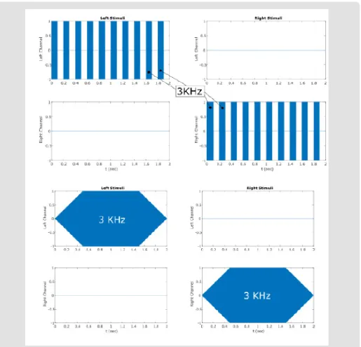
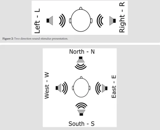
Two classes of 2 secs stimuli were applied randomly. The first is a pure tone of 3 kHz with 500 ms increasing tone, steady during 1 second, and then decreasing tone during 500ms. The second stimulus was a burst of 3 kHz pure tone with durations of 100ms ON, and 100ms OFF for 10 trials. This give a total of 224 auditory stimuli (112 right/112 left). Each series of 16 stimuli takes around 2 minutes and the participant is allowed one minute to rest between trials. The sound stimuli were presented through a program written in Matlab (Figure 1). The National Instruments device was used to put markers in the EEG data as they were recorded simultaneously when auditory stimuli were presented. The results presented in this paper are from the analysis of EEG data collected from 3 different subjects. Apart from 2 directions of Left and Right for sound stimulus presentation, four direction stimuli were also presented to the subjects. For the four direction sound data presentation, we used sound localization using the head related transfer function. The Head Related Transfer Function (HRTF) is a novel technique to simulate direction of arrival of sounds. Head Related Transfer

Function (HRTF) is also called as transfer function from the free field to a specific point of the ear canal. In mathematical terms the transfer functions for Left and Right are shown below:

(

, , ,

)

(

, , ,

)

/

(

,

)

L L L o

H

=

H r

θ ψ α

=

P r

θ ψ α

P r w

(

, , ,

)

(

, , ,

)

/

(

,

)

L L R o

H

=

H r

θ ψ α

=

P r

θ ψ α

P r w

respectively. The Head Related Transfer Function (HRTF)

are functions of distance between source and center of the head r, and the parameters of the function are: the source angu -lar position θ, the elevation angle

ψ

w

the equivalent dimension of the head α. Figures 2 & 3 show the di -rectional sound stimulation implementations using Head Related Transfer Function (HRTF).

Figure 2: Two direction sound stimulus presentation.

Time-Frequency Analysis

The 32 channel EEG data collected are pre-processed using band-pass filtering to remove low frequency noise, artifacts due to eye blinks and hardware induced artifacts. In order to extract mean

-ingful features from signals for source identification, it is necessary to map data in overlapping feature spaces to a separable space by high dimensional feature mapping. This increases the dimension

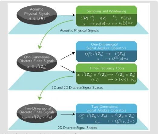
-ality of the feature space, but the classes are easily separable in this space, and linear classifiers can be used to classify the data in this high dimensional space. In this project, we have mapped 1-D signal spaces to 2-D signal spaces through timefrequency methods (TFM). The group of signals taken from the electrodes on the scalp are in the space of continuous physical signals L R( ) _{Figure 4. These} sequences are the mapping from L R( )to l Z( )through an analog to digital process. The sampled/quantized version is computing us

-ing a window operator that transform l Z

( )

( )

experiment is conducted. These signals now are in _{l N}2

( )

and is the

space of discrete finite signals with finite energy. EEG signals can be processed by a computer using time-frequency tools to map the

signals from space 2

( )

l Z to the space 2

(

)

l Z ×Z _{. The increased}

dimensionality of the signal space reveals more information about the original signal. The mapping from 2

( )

(

)

N N N

l Z →l Z ×Z _also ad-ditional computations while processing the EEG signal analysis in the transformed space. In multiway signal-processing the selection of efficient and optimal methods for the processing of electroen

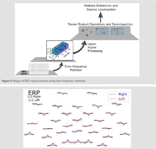
-cephalographic signals is a problem addressed by many authors [5-7]. Figure 5 shows the stages or levels of neural signal analysis presented in this paper. Time-frequency methods allow the obser

-vation of details in signals that would not be noticeable using a tra

-ditional Fourier transform. One of the problems of conversion to time-frequency spaces is that, according to the length of the input signal, the conversion can be time, and memory consuming. The two methods for time frequency analysis considered here are the Short Time Fourier Transform (STFT), and the Wavelet Transform

(WT) Figure 6.

Figure 5: Stages of EEG signal analysis using time frequency methods.

Figure 6: Shows the EEG ERP responses to 2 direction auditory stimulation. Time Domain Event-Related Potentials for Auditory Stimuli N=112 Right and Left.

Short Time Fourier Transform Analysis

The STFT has been a widely used time-frequency signal processing operator. The Cyclic Short Time Fourier Transform (CSTFT) has certain advantages over STFT that are mentioned below.

Short Time Fourier Transform Definition: Given a signal

[ ] ( )

x n l Z∈ _{and let} w n l Z

[ ] ( )

rectangular window function, the STFT is defined as follows:

[

,

]

[ ] [

]

n

X m k

x n w m n e

=∞

= ∑

−

A special variation of STFT is the cyclic short time Fourier transform. The CSTFT is a STFT with a window function w n

[ ]

performs a cyclic shift with the

m n

−

m n

−

Cyclic Short Time Fourier Transform Definition: Given

a signal x n l Z

[ ]

( )

[ ] ( )

function, the CSTFT is defined as follows:

[

]

[ ]

, ,

N

kn

x v N N

n Z

S m k x n w m n W ∈

 

=

∑

(2)

where, kn jN2 ( )

N

W =e− π kn , m Z∈ N (time shift) and K Z∈ N (frequency

axis). The CSTFT makes a mapping from the space L Z( )N to the

from the signal space l Z( N×ZN)to the signal space l Z( N×ZN).

This ensures that the mapping is constant, independent of the length of the input signal because through, a different segmentation, it can be ensured that the conversion falls into the same signal space. The new signal space gives richer information. A special group of the STFT is the Gabor transform, a generalized version is given in Equation 3. This time-frequency transform uses a window defined as a Gaussian function.

( )

_,

( )

G t f

e

e

x

_{τ τ}

d

−∞

=

_∫

Continuous Wavelet Transform and Discrete Wavelet Transform

Wavelet Transform is based on a group or class of translated and dilated functions called wavelets. The continuous wavelet functions are defined in Blu et al. [8] as:

( )

, 1

t a t t_at

a

ψ = ψ_ − _

  (4)

And the CWT is defined based on these wavelets.

( )

( )

CWT t a x t dt x

a ψ

∞

−∞

−

=

_∫

The CWT gives a time frequency representation in terms of delay and dilation. The CWT representation has advantages over the CSTFT at low frequencies. In EEG, the presence of information

at low frequency is very common. Therefore, CWT is better than the CSTFT for EEG time frequency analysis.

Feature Extraction and Classification

The algorithm for feature extraction and classification using a support vector machine (SVM) classifier is shown in Figure 7. Time Frequency Method (TFM) is either the CSTFT or the CWT. The 32 channel EEG data were organized as tensors [9-12] and the time frequency methods were implemented in Python and visualized us

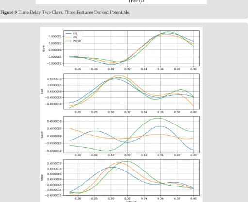
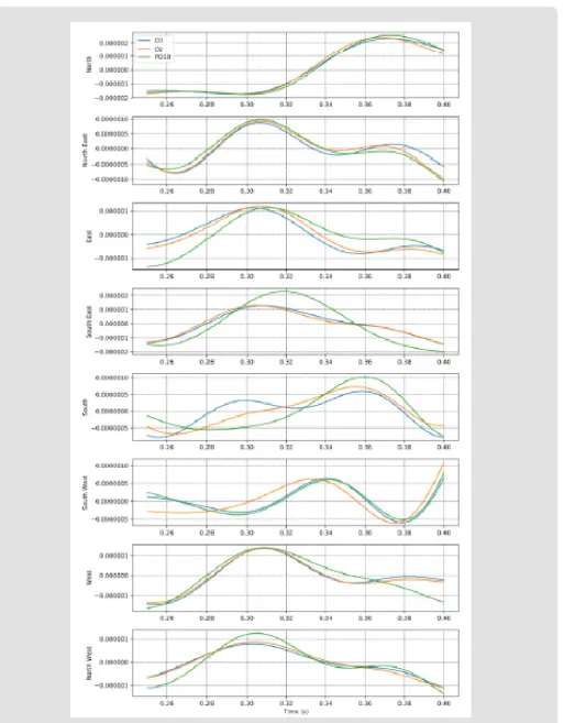
-ing MNE [13-15]. The EEG data of 112 trials is divided in to 56 for trials for training and 56 trials for testing. 40 random trial averaging was done for training and testing of the SVM classifier. The results for two subjects is shown in Table 1. Figure 8 shows the ERPs for 3 EEG channels that are from the frontal and temporal regions of the brain involved in processing of auditory stimulus. The time delay in these evoked potentials can be clearly seen. Similarly, Figures 9 & 10 shows the time delays in the evoked potentials for a 4 and 8 di

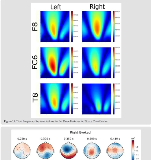
-rection auditory stimulation, respectively. In this case, the occipital and parietal lobes are involved. This shows that as more complex sounds are presented, different neuronal pathways are activated in processing these auditory stimuli. Figure 11 shows the time fre

-quency representation for the 3 features for the 2 direction audi

-tory ERPs. Figure 12 shows the topo plots for the EEG signals re

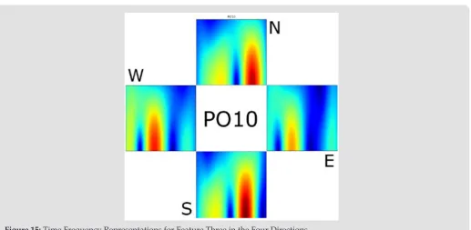
-corded during left and right direction auditory stimulation. Figures 13-15 shows the time frequency representation for the 3 features for the EEG signals evoked by auditory stimulation in 4 directions.

Figure 8: Time Delay Two Class, Three Features Evoked Potentials.

Figure 11: Time Frequency Representations for the Three Features for Binary Classification.

Figure 13: Time Frequency Representations for Feature One in the Four Directions.

Figure 15: Time Frequency Representations for Feature Three in the Four Directions.

Results

Table 1 shows very good accuracies for source localization when two directions auditory stimulus are presented. For the 4-direction case, in Table 2 it can be seen that the classifier has difficulty in identifying the South direction. The salient features from the CWT in each of the neuronal regions for multiple direction auditory stimulation can be seen from the time frequency representations. The CWT features performed well for 4 directions auditory stimulus

localization. As can be seen, results for 2 directions is close to 100%.

The time delay plots in Figures 9 & 10 show that for more source directions, neuronal signals from the occipital and parietal regions have higher discriminatory power than frontal or temporal regions.

Table 1: Confusion Matrix 2 Class Using SVM Classifier for 3

Subjects.

L (W) R (E)

L (W) 100% 0.10%

R (E) 8% 92%

L (W) R(E)

L (W) 88% 12%

R(E) 15% 85%

L (W) R (E)

L (W) 100% 0.00%

R (E) 0.00% 100%

Table 2: Confusion Matrix for4 Class Using SVM Classifier.

N E S W

N 100% 0% 0% 0%

E 0% 82% 0% 18%

S 35% 1% 27% 38%

W 0% 4% 0% 79%

Conclusion

Auditory processing in the brain was analyzed using time frequency analysis of EEG signals acquired from the brain during sound stimulus presentation. The results show that as number of source directions is increased, different regions of the brain are involved in processing the signals. This implies that as sound becomes more complex such as in speech, music, and language perception, higher intricate auditory pathways in the brain are involved in processing and decoding these sound patterns. The comparison of the time domain vs time-frequency domain factorization of EEG shows that increasing the dimensionality of the EEG signals, provides a better way to discriminate the ERP of

auditory stimuli and localize sources. Apart from sound direction

localization from EEG, it is evident that EEG can also be used

as a neuroimaging modality for understanding and decoding

sensory and motor functional pathways in the brain. This work can be extended to analyzing complex music, speech and language perception in the brain.

References

1. I Nambu, M Ebisawa, M Kogure, S Yano, H Hokari, et al. (2013) Estimating the intended sound direction of the user: toward an auditory brain computer interface using out of head sound localization. Plos One 8(2). 2. S Makeig, TP Jung, AJ Bell, D Ghahremani, TJ Sejnowski, et al. (1997) Blind

separation of auditory event-related brain responses into independent components. Proc Nat Acad Sci 94(20): 10979-10984.

3. A Bednar, FM Boland, EC Lalor (2017) Different spatio-temporal electroencephalography features drive the successful decoding of binaural and monaural cues for sound localization. European Journal of Neuroscience 45(5): 678-689.

4. T R Letowski, S T Letowski (2012) Auditory spatial perception. ARL-TR-6016.

two-way to multitwo-way component analysis. IEEE Signal Processing Magazine 32(2): 145-163.

6. T Alotaiby, FEA El Samie, S A Alshebeili, I Ahmad (2015) A review of channel selection algorithms for EEG signal processing, EURASIP Journal on Advances in Signal Processing 1(66).

7. E C van Straaten, C J Stam (2013) Structure out of chaos: Functional brain network analysis with EEG, MEG, and functional MRI. European Neuropsychopharmacology 23(1): 7-18.

8. T Blu, J Lebrun, Linear (2010) Time-Frequency Analysis II: Wavelet- Type Representations. ISTE 93-130.

9. C Boutsidis, E Gallopoulos (2008) SVD based initialization: A head start for nonnegative matrix factorization. Pattern Recognition 41(4): 1350-1362.

10. F Cong (2016) Nonnegative Matrix and Tensor Decomposition of EEG. 09: 275-288.

11. A Cichocki, R Zdunek, AH Phan, S Amari (2009) Nonnegative Matrix and Tensor Factorizations: Applications to Exploratory Multi-way Data Analysis and Blind Source Separation. John Wiley Sons Ltd 2009. 12. T G Kolda, B W Bader (2009) Tensor decompositions and applications.

SIAM Rev 51(3): 455-500.

13. A Gramfort, M Luessi, E Larson, D Engemann, D Strohmeier, et al. (2013) MEG and EEG data analysis with MNE-Python, FrontiersinNeuroscience 7: 267.

14. F Pedregosa, G Varoquaux, A Gramfort, V Michel, B Thirion, et al. (2011) Scikit-learn: Machine learning in Python. Journal of Machine Learning Research12(2011): 2825-2830.

15. J Kossaifi, Y Panagakis, A Anandkumar, M Pantic (2018) Tensorly: Tensor learning in python. CoRR vol. abs/1610.09555.

Submission Link: https://biomedres.us/submit-manuscript.php

Assets of Publishing with us

• Global archiving of articles

• Immediate, unrestricted online access • Rigorous Peer Review Process

• Authors Retain Copyrights

• Unique DOI for all articles

https://biomedres.us/ This work is licensed under Creative

Commons Attribution 4.0 License

ISSN: 2574-1241

DOI:10.26717/BJSTR.2019.19.003362