Optimization of Turbine and Heat Exchanger Stages For the Expansion Process of a Compressed Air Energy Storage System (Fortran Computer Modeling and Simulation).

(1)

ABSTRACT

NICKELS, JOHN THOMAS. Optimization of Turbine and Heat Exchanger Stages For the Expansion Process of a Compressed Air Energy Storage System (Fortran Computer Modeling and Simulation). (Under the direction of Dr. Stephen Terry, PE).

Electricity production is one of the pillars supporting our modern world. Through careful planning and quick action, power producers keep the steady stream of electrons flowing through a seemingly endless network of transmission and distribution lines. Somewhat unpredictable, grid loads are supplied by base, intermediate, and peak generation plants. In order to supply all system loads reliably, energy producers may produce more energy than necessary, or may use quicker, more expensive electricity generation methods. Energy storage is seldom incorporated into an electricity grid’s framework, particularly on a utility scale. Storage allows for, among other things, more predictable generation, less wasted resources, reserve capacity, electricity time shift, frequency regulation and intermittency remediation for renewable generation. The energy storage currently implemented generally takes the form of pumped hydropower, a geology-dependent technology, or as electrochemical battery storage, which can be very expensive with shorter longevity. New technologies are being studied and new projects are being constructed. An old technology that has been both studied and implemented is compressed air energy storage (CAES). Only a handful of facilities exist around the world, with the two oldest using the stored compressed air for combustion turbine-based electricity generation. The computer model written and run for the purpose of this Master’s thesis simulates a compressed air energy storage system. The CAES system is

(2)

(3)

(4)

Optimization of Turbine and Heat Exchanger Stages for the Expansion Process of a Compressed Air Energy Storage System

(Fortran Computer Modeling and Simulation)

by

John Thomas Nickels

A thesis submitted to the Graduate Faculty of North Carolina State University

in partial fulfillment of the requirements for the degree of

Master of Science

Mechanical Engineering

Raleigh, North Carolina

2015

APPROVED BY:

_______________________________ ______________________________

Dr. Stephen Terry, PE Dr. Herbert Eckerlin, PE

(5)

DEDICATION

(6)

BIOGRAPHY

John was born on September 29, 1976 to Marilyn and Kenneth Nickels in our Nation’s Capital, the District of Columbia. His older brother RJ was ecstatic to have a brand new punching bag, as his old one was worn and full of tiny fist holes. By the time John was four, he had already deduced that he was likely the milkman’s son, as he looked nothing like any of his relatives

and was not anywhere as smart as them. I mean, seriously, he could not even tie his own shoes. Thankfully for little Johnny, Velcro was finally applied to shoes, sparing him from endless embarrassment. Due to his inherent intolerance of anything dairy-related, he was forced to give up his lifelong dream of following in his biological father’s footsteps of dairy logistics, and chose instead to study the lucrative field of environmental biology. This education decision landed him in the ever expanding and high stakes field of water and soil testing, a career that is much sought after by peanut butter and jelly connoisseurs and ramen enthusiasts alike. It was only because he was making too much money that he decided to take an early retirement to explore his one true love, Mechanical Engineering. Sorry honey. He had given up his fleeting flirtations with the field during his childhood in Maryland over the lack of engineering schools that did not have some silly turtle for a mascot. Because seriously, a turtle? Why not a rock? It would probably be faster. Not that a Wolfpack is any better for a mascot. That is like calling a team a “swarm” instead of “the bees.” Sure, both are scary, but the bees are what sting you. Anyway, it was only when John moved to North Carolina that he realized there were engineering schools that had somewhat logical mascots. It was at this point of recognition that John decided to throw his cares to the wind, move to Raleigh, and study to be a Mechanical Engineer……with cool robot arms and computer chip brain parts!

(7)

ACKNOWLEDGMENTS

For my family, I would first like to acknowledge and thank my lovely wife, Anna, for her overwhelming patience and support throughout my extended return to education; you are truly the backbone of our happy little family. I want to thank my son Jude, not only for being THE BBE, but for reminding me of the reasons to stay on my path; thanks little dude! I would also like to acknowledge my parents, Ken and Marilyn, for their unwavering commitment to and belief in education; I could not have survived without your experience, advice and support. To that, I must mention my late grandfather and grandmother, Frank and Rita Wenzke; without their commitment to education and family, none of this endeavor would be possible. Finally, I would like to acknowledge my older brother RJ. You started this thing, and have been my model for success; you are truly the smartest person I have ever met.

Next, I would like to acknowledge Jackson Wooten, Daniel Poprocki, Kiran Thiruman, Corey Misenheimer, Taylor Atkins, Gopal Chaudry, Alex Viola, Harsha Ramakrishna, Kevin Martin, Josh Poole and Panth Naik. You guys put up with me for far too long; thanks for not kicking me out of the IAC office, even though I know you wanted to. Thanks also to Mike Breedlove, for giving me a shot in the shop, Dr. Paul Ro, for giving me a spot in your lab, and to Annie White for taking SO MUCH time to help; you are all awesome. Thanks to Dr. James Kribs, for your sanity checks and derivations; I’m glad you came back to State just to help me! Ha.

Ha. Ha.

I would also like to acknowledge the Idaho National Laboratory for the opportunity to work on the energy storage project that initialized the research for this thesis. It is a noble task to push progress forward, and it is only with the determination to recognize and realize innovative ideas that future generations might thrive.

(8)

board as a research assistant and your patient support throughout this endeavor; you are worth more than you know, and you know more than most. Thank you, Dr. Eckerlin, for your support, help, and unbelievable wealth of knowledge; you have spilled more engineering concepts on your tie than we can ever learn. Thank you, Dr. Saveliev for your commitment to the thermal sciences and to teaching; your humor, inquisitive nature, and capacity for understanding have been models for me during my studies and my research. I value your perspectives because you see things so completely. All three of you are exceptional teachers and remarkable people; I hold you all in the highest esteem and am so honored for you to be part of this.

(9)

LIST OF TABLES

Table 1: Air Compression Variable Values Used for All Simulations ... 76

Table 2: Turbine Stage Number and Temperature Gradient Variations ... 88

Table 3: Turbine Inlet Pressure Variations ... 98

Table 4: Storage Pressure Variations ... 103

Table 5: Storage and Turbine Input Pressure Variations ... 107

Table 6: Turbine Mass Flow Rate Variations ... 113

Table 7: Dew Point Temperature Variations ... 118

Table 8: Compressor Variable Values ... 122

(12)

LIST OF FIGURES

Figure 1: Electricity Generation Allocation for System Demand (Summer Day) [Load Curve

Data [1]] ... 2

Figure 2: System Demand by Customer Class [Load Data [1]] ... 6

Figure 3: Electricity Generation by Fuel Source 2013 (EIA)[5]... 7

Figure 4: Electricity Generation by Fuel Source (EIA)[5] ... 8

Figure 5: Rankine (Steam) Cycle, T-s Diagram[8] ... 9

Figure 6: Open Brayton (Gas) Cycle[8] ... 10

Figure 7: Full Generation and Demand-Driven Generation [Load Data [1]] ... 13

Figure 8: Pumped Hydro Storage Cycle[15] ... 15

Figure 9: Positive Displacement Compressor Types ... 20

Figure 10: Reciprocating Piston-Cylinder Compression[24] ... 21

Figure 11: Helical Screw Compression (Dark Areas Are Air)[25] ... 22

Figure 12: Siemens STC-SX Axial Compressor[26] ... 23

Figure 13: GE Centrifugal Compressors (Closed and Open Impeller Designs)[27] ... 24

Figure 14: OPRA 016 Radial Gas Turbine (With Centrifugal Compressor)[28] ... 25

Figure 15: Centrax CX400 Axial Gas Turbine (With Axial Compressor)[29] ... 26

Figure 16: Basic Compressed Air Energy Storage System Components and Layout ... 31

Figure 17: P-v Diagram of Isothermal, Polytropic and Isentropic Compression[7] ... 36

Figure 18: Staged Intercooled Compression System with Aftercooling ... 39

Figure 19: Staged Compression with Intercooling (Polytropic Processes Shown)[7] ... 41

Figure 20: Insulated Storage Receiver Diagram ... 46

Figure 21: Staged Heated Expansion System (Turbines & Heat Exchangers) ... 48

Figure 22: Compressed Air Energy Storage Sizing and Runtime Program ... 55

Figure 23: Excess Power vs. Time (Peak Day) ... 80

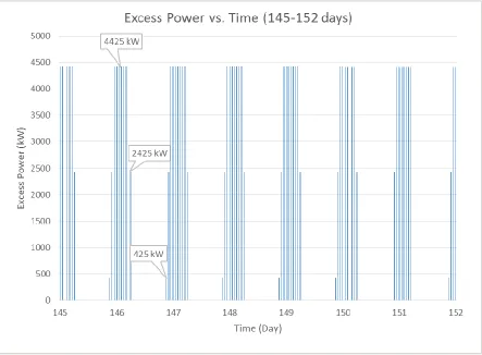
Figure 24: Yearly Excess Power vs. Time (Day 145-152) ... 81

Figure 25: Receiver Mass In/Out & Total vs. Time (Day 0-7)... 83

Figure 26: Receiver Mass In/Out & Total vs. Time (Day 179-186) ... 84

Figure 27: Receiver Temperature & Pressure vs. Time (Day 0-7) ... 85

(13)

Figure 29: Receiver Temperature & Pressure vs. Time (Day 182-183) ... 87

Figure 30: Reheat Energy and Receiver Temperature vs. Time (Day 182-183) (Tout=300 K) ... 89

Figure 31: Reheat Energy and Receiver Temperature vs. Time (Day 179-186) (Tout=Tdp) ... 90

Figure 32: Reheat Energy and Receiver Temperature vs. Time (Day 179-186) (MAX Reheat .. 91

Figure 33: Tin, Tout, % Input Return and Δh vs. Stages (SIZE MODEL) (Full Reheat) ... 92

Figure 34: Tin, Tout = 300 K, % Input Return and Δh vs. Stages (SIZE MODEL) ... 93

Figure 35: Tin, Tout = Tdp, % Return and Δh vs. Stages (SIZE MODEL)... 94

Figure 36: Energy Payback, Reheater Size & Power Output vs. Stages (Full Reheat ... 95

Figure 37: Energy Payback, Reheater Size & Power Output vs. Stages (Reheat for Tout=300 K) ... 96

Figure 38: Energy Payback, Reheater Size & Power Output vs. Stages (Reheat for Tout=Tdp ) . 97 Figure 39: Minimum and Required Volume vs. Turbine Inlet Pressure (Tout=300 K) ... 99

Figure 40: Receiver and Turbine Temperature Limits vs. Turbine Inlet Pressure (Tout=300 K) ... 101

Figure 41: Input Return and Power Out vs. Turbine Inlet Pressure (Tout=300 K) ... 102

Figure 42: Minimum and Required Receiver Volumes vs. Storage Pressure ... 104

Figure 43: ṁmax and Total Mass (SIZE MODEL) vs. Storage Pressure ... 105

Figure 44: Input Return and Power Out vs. Storage Pressure ... 106

Figure 45: Minimum and Required Receiver Volumes vs. Storage Pressure (ΔP 10 bar) ... 108

Figure 46: Max Receiver Temperature and Pressure vs. Storage Pressure (ΔP 10 bar) ... 109

Figure 47: ṁmax and M (SIZE MODEL) vs. Storage Pressure (ΔP 10 bar) ... 110

Figure 48: Input Return and Power Out vs. Inlet Pressure (ΔP 10 bar) ... 111

Figure 49: Turbine Inlet and Outlet Temperatures vs. Storage Pressure (ΔP 10 bar) ... 112

Figure 50: Stored Energy vs. Mass Flow Rate ... 114

Figure 51: Reheat Required vs. Mass Flow Rate ... 115

Figure 52: Reheat Required vs. Mass Flow Rate (7.125 kg/s) ... 116

Figure 53: Stored Energy vs. Mass Flow Rate (7.125 kg/s) ... 117

Figure 54: Water Removed vs. Inlet Dew Point Temperature ... 119

Figure 55: Tin and Tout vs. Stages (Tout=Tdp) ... 123

Figure 56: Expansion System Output and Reheat Power vs. Stages ... 124

(14)

(15)

CHAPTER 1

Introduction

Electricity is a mainstay of our technologically advanced civilization. Economies and lives depend on the steady flow of electrons through a seemingly endless matrix of metal strands. Many of the Earth’s six billion occupants take this flow for granted, to power anything from heavy machinery on the factory floor to life support systems in an emergency room; few of them may recognize the lifetimes of technological developments and tremendous amounts of effort that go into the generation, transmission, and distribution of this essential utility. Electricity use and demand drives electricity production. Power must be produced and supplied when it is required, instantaneously and without fail. This requires major infrastructure which includes, among other things, generation plants, miles of power lines for transmission and distribution, transformers, metering and monitoring equipment, and occasionally, energy storage reserves.

(16)

Figure 1: Electricity Generation Allocation for System Demand (Summer Day) [Load Curve Data [1]]

(17)

to design and analyze a compressed air energy storage (CAES) system model, and to optimize the number of turbine-heat exchanger couple sets for the expansion process.

The general outline of this thesis paper is:  Chapter 1: Introduction and Background

The first chapter will set the stage for the rest of the paper. It explains the reasons for creating the model, the current state of the art for compressed air energy storage and the physical components considered in the model.

 Chapter 2: Relevant Thermodynamic Theory

The second chapter is devoted to theory, and explains the relevant scientific principles regarding air compression, storage and expansion. These are the thermodynamic foundations of the model.

 Chapter 3: Model Description

Chapter three outlines and explains all of the components, key variables, and concepts of the computer model. This section details the overall construction and flow of the program, as well as the individual subroutines.

 Chapter 4: System Analysis and Results

The purpose of chapter four is to explain the way the model was used, the specific variable changes that were made, and their output. The effect on number of turbine/heat exchanger couples is the focus. Overall results as well as those attributed to individual component (variable) augmentation are explored and analyzed.

 Chapter 5: Final Simulation, Discussion and Conclusions

(18)

Background

1.1 Energy Production, Consumption and Demand

Two important concepts relating to energy use and production are consumption and demand. The primary “take-away” concept is that consumption is an amount, while demand is a rate. This difference can be explained with an analogy of a water fountain versus a fire hose. Both devices require water, but they require it at different rates. To deliver water to the end-user, a fire hose requiressignificantly more water every second it operates than a water fountain does; this is the concept of DEMAND. If you send the amount of water intended for the fountain to the fire hose, you will never put out your fire (unless it is very small). If you reverse the scenario, you may just blow your drinking fountain off the wall. Regardless of the arrangement, the water utility delivering the water to the two customers must be able to supply ALL of the system’s customers at the TOTAL COMBINED DEMAND RATE at the time it is needed. If the system is below capacity, fires may continue to burn as hoses trickle.

The concept of consumption is much simpler. It is merely the AMOUNT used during a certain time period. It is a count, not a rate. Given sufficient time, the water fountain can consume as much or more water than the fire hose. For example, if a fire hose that requires 5 gallons per second to operate (DEMAND) is left fully open for one hour (3600 seconds), it will CONSUME an amount of 18,000 gallons. If a water fountain that requires 0.05 gallons per second to operate is left on for 100 hours (360,000 seconds), it will also consume an amount of 18,000 gallons. The periods over which the water is used are quite different, but the total consumption is the same.

(19)

merely a bookkeeping practice to make dealing with power and energy easier. Since kilowatts are really just kilojoules per second:

kJ ENERGY kW

s TIME

 

 _{ } _

 

and kilowatt-hours are really just the number of kilojoules per second (kW) used for a period of time in hours (3600 seconds per hour):

ENERGY kJ

kWh hours TIME ENERGY

s _TIME

 

  _   _

 

The units match up. Demand (power, kW) is what drives the scale of production capacity (system infrastructure). Consumption (energy, kWh) is the sum of the actual individual system demands over a period of time, which drives the degree to which a system is used (fuel use). Now that we understand demand and consumption, we can tackle system loads.

(20)

Figure 2: System Demand by Customer Class [Load Data [1]]

(21)

ecosystem[3][4]. Time will tell the outcome, though reliable, zero-emissions and low cost electricity is a difficult position to argue against.

(22)

Figure 4: Electricity Generation by Fuel Source (EIA)[5]

Immense planning goes into the application and operation of these generation technologies. Since all of the demand at any given point must be met, the power generation capacity must exist to handle it. Different loads must be handled by different components of the generation infrastructure. It would not make sense to have gas turbines handling the base load while a nuclear plant cycles up and down to handle peak demand. This would be unnecessarily costly and could possibly damage the nuclear fuel rods. Since system loads are never known before they occur, power producers must make highly-educated guesses as to how much power to produce and when. To say the guessers, or system operators, have gotten better at guessing, or dispatching[6] would be a colossal understatement. Electric utilities have a myriad of strategies they use to predict, plan and produce, in order to meet the needs of every customer.

(23)

1.2 Electricity Production and Power Cycles

Electricity for consumer end-use is produced in much the same way as it was a century ago: an electric generator is turned by some mechanical means. This often reduces to a choice between two basic power cycles: The Rankine Cycle and The Brayton Cycle. The Rankine Cycle[7], Figure 5 below, involves heating water (or another working fluid) until evaporation, which increases the temperature and pressure of the working fluid. Oftentimes the fluid is superheated, which increases the fluid’s ability to do useful work. This hot, high pressure vapor is expanded through a vapor expansion turbine which in turn produces the radial motion used to drive an electrical generator. The Brayton Cycle[7], conversely, involves compressing a gas, heating that gas, and expanding the hot high pressure gas through a gas expansion turbine, shown in Figure 6. In many applications, the gas is air which is heated via combustion with a fuel; the exhaust gases produced are sent through the turbine. Again, this expansion process produces the radial motion that drives an electricity generator.

(24)

Figure 6: Open Brayton (Gas) Cycle[8]

(25)

1.3 Finite Resources, Renewables, and Conservation

Hydropower, wind, solar thermal and semiconductor-based energy generation are power production technologies that have no fuel costs associated with energy generation. After they are manufactured, constructed and implemented, nothing has to be combusted to make them work. They are commonly referred to as renewable energy sources. Despite the fact that the energy input for their operation is transferred or transformed, the medium of energy transmission remains (neglecting any long-term degradation effects) unchanged. Air carries kinetic energy as wind, water carries the potential energy of an elevation, and photons are pure electromagnetic radiation. Unfortunately, the wind does not always blow, the sun does not always shine and the rain does not always fall. This is another major reason to incorporate utility-scale energy storage. Inherent in many of these sources of “free-energy” are these production reliability and intermittency issues. Add to this the environmental impacts of construction and operation of these installations, water and land use concerns, and a growing pile of political and economic issues. The result is a considerable mess of problems that need solutions. This is not to say that these technologies should be disregarded; rather they should be as carefully considered as any other potential generation technology.

(26)

emissions. Finally, many products of combustion are harmful to the health of humans and to the environment. Sulfuric acid, carbon monoxide, soot/ash, uncombusted fuel and nitrogen oxides are but a few contaminants that can pollute our environment, from which we are inseparable[10].

These benefits and liabilities of renewables and non-renewables are merely snowflakes on the tip of an iceberg of economic, scientific and political issues that are tied to energy use and production. In the end, one of the most effective means of alleviating the maladies caused by energy production is simply to use less energy; to conserve. New technologies, designs and practices, such as LED lighting, “green” building methods, and occupancy-based energy use allow us to use but a fraction of the electricity we once needed to perform the same functions. Every day, more people around the world are using electricity[11], making energy conservation through innovation crucial to our energy future. In the future, the question may not be, “how much can we produce?” but “how little can we use?”

1.4 System Loads and Energy Generation

(27)

Figure 7: Full Generation and Demand-Driven Generation [Load Data [1]]

Generation facilities try to optimize production, but electricity demand fluctuates. Large base load facilities seldom scale back their operations significantly when the system load is lower than the base/intermediate load energy production level. It is simply less costly to run at a higher fire than to reduce or shut down production temporarily, only to have to ramp up operations again. Unfortunately, this leads to excess energy capacity or production during these “off-peak” periods. This “off-peak” energy is often sold at much lower rates than during “on-peak” periods. If this energy could be stored, it could be sold during the “on-“on-peak” period,

(28)

1.5 Energy Storage and Capacity

(29)

Figure 8: Pumped Hydro Storage Cycle[15]

Obviously and for good reason, economic feasibility dominates the decision-making process for any potential business venture. This holds just as true for the utility sector as it does for any other sector. If a technology is not energy-dense, cost-effective, and reliable with a long life span, it will not likely pass muster for an electric utility. Why would a utility even consider mechanical storage when chemical storage is readily available? They certainly have energy and power densities worth considering[2]. However, despite incredible breakthroughs in chemical battery technology over the years, the longevity of most chemical batteries is terribly lacking[16][17]. The lifecycle of chemical batteries is nowhere near those of pumped hydro, flywheel, or compressed air systems. If the life span of the installation is not more than ten years, the overnight costs will have to be quite low to justify the disposal costs for a fleet of dead batteries. Unfortunately, many energy-dense chemical batteries have a high per unit cost[18] as well as significant issues of environmental impact and energy use during manufacture[19]. Despite this, all forms of energy storage, whether they are mechanical, chemical or biological, should be researched and explored. The criteria requirements for any storage project, now and in the future, will include capacity, longevity, costs and payback.

(30)

1.6 The Current State of Compressed Air Storage

Compressed air has been widely used since the late 19th century, starting with mining and metal manufacturing[20]. Indeed many of the early air compressors predate the advent of electrical power, and were driven by steam engines. These systems did not necessarily incorporate receivers (vessels) to store compressed air. Despite this, storing energy with compressed air is, without doubt, not a new idea. In fact, all compressed air systems that make use of air receivers are by their nature energy storage systems. Energy is input to the mechanical system that compresses the air. This pressurized air is sent to a receiver for later use, capable of being transferred over distances via conduit. When called upon, the air is allowed to expand in a controlled manner to some lower pressure, usually through a pneumatic tool or device to perform a task.

The concept of using air to store excess energy for electricity generation is not new either. The first commercial utility-scale compressed air energy storage facility (CAES), still currently operating, was opened in Huntorf, Germany in 1978[21]. It stores off-peak energy as compressed air (up to 100 bar) in two solution-mined salt caverns with total volume of 310,000 m3. It has a rated capacity of 321 MW and can operate for 2 hours. Generation is used to supply peak loads, supply a “spinning reserve” for grid system backup, and to ameliorate supply and

demand fluctuations on the grid (frequency regulation). Huntorf is capable of going from an offline state to producing at full capacity without grid power (black start), in six minutes. This compressed air is used to feed the combustion and expansion processes of gas turbines.

(31)

chamber. This allows the turbine to output more power to the generator, as no power needs to be devoted to compress air. This thirty-six year-old facility touts a 42% round-trip cycle efficiency for compression, storage and expansion.

The next-oldest CAES plant in operation is located in McIntosh, Alabama, and has been in service since 1991[21]. Like the Huntorf facility, the PowerSouth CAES installation stores compressed air (up to 76 bar) in a 283,000 m3_{solution-mined salt cavern. “Why a salt cavern?”}

you may ask. Water can be pumped into a salt bed formation to dissolve the salt, and the salt solution is pumped out leaving a void in the bed. Once the desired volume is dissolved away, the cavern is allowed to dry and seal itself back up, leaving an airtight, underground vessel[22]. The generation system at McIntosh also uses a gas turbine for the expansion process, but is rated for 110 MW and can run for up to 26 hours; it is used to supply peak loads and can serve as a spinning reserve. McIntosh makes use of a heat recovery system to preheat the cold compressed air with the turbine exhaust, which decreases fuel use by 25%.

The third CAES plant to come online is located in Gaines, Texas, and uses technology designed by General Compression, Inc.[21]. The 2 MW plant stores excess energy, also in a salt cavern, produced by wind turbines using proprietary “near isothermal” air compression technology.

The rated run time for storage output is 250 hours. Unlike the facilities at Huntorf and McIntosh, the expansion system does not involve combustion of any fuel. The expansion process also uses proprietary “near isothermal” technology. This means that except for system losses, input energy is not lost as heat during the compression stage of the storage cycle. This is quite important, as isothermal or near isothermal compression and expansion are the “holy grail(s)” of CAES; if they can be performed quickly, reliably, and with acceptable roundtrip

(32)

Other projects under construction or in the planning stages include[21]: a 200 MW, 5 hour adiabatic CAES system in Staßfurt, Germany that stores the heat removed during compression which will be added back prior to expansion; a 300 MW, 10 hour adiabatic CAES system in San Joaquin County, CA that will use an old natural gas reservoir for air storage; a 9 MW, 4 ½ hour CAES system in Queens, NY that uses steel piping as the storage receiver; and two 1 MW underwater compressed air energy storage (UCAES) facilities, one 5 m offshore from Toronto, ON in Lake Ontario, the other off the coast of Aruba. The Hydrostor demonstration facility in Canada will be able to run for 4 hours, and the facility in Aruba will run for 8 hours. Both systems will compress air with excess energy produced by wind turbines. These systems are unique in that they use inflatable receiver bladders and the hydrostatic pressure of the water column above them to store the air at a constant pressure. Finally, a 1.5 MW, 1 hour Isothermal CAES demonstration system manufactured by SustainX Inc. is in operation at the company’s headquarters in Seabrook, NH. This system, according to the manufacturer, compresses air isothermally by spraying water into the compression system (piston) to absorb heat. This hot water is stored along with the air and the water is used to heat the air prior to the expansion process. This and Hydrostor’s systems will not use fuel in the expansion process, using only the heat removed from compression to reheat the air.

(33)

1.7 Turbomachinery and Receivers

This purpose of this section is to give the reader a basic overview of the components included in the system. The components present in the modeled system are intercooled/aftercooled compressors, adiabatic tanks, and expansion turbines with interstage heat exchangers. All generators, motors, wiring, electronics, controls, switches, piping, valves, metering equipment and structural components that will need to be considered for a full implementation were not considered here; these must be included in future, more complex modeling and simulation versions if major decisions are to be based on this model.

1.7.1 Compressors

Gas compressors do one thing: they bring physically push the molecules of the gas closer together, changing its volume. The same amount of mass that used to take up a larger volume can now fit into a smaller volume, increasing the mass density (ρ, [kg/m3]), or decreasing the specific volume (υ, [m3/kg]), which are two sides of the same coin. Compressors do not necessarily increase the pressure of the gas, as heat can be removed which will lower the temperature. This will lower the pressure if the compressed volume remains constant. All compressors have some motive force, such as a driveshaft, and some energy input to supply the force; the work input pushes against the air that wants to expand. Compression can be accomplished in a number of ways, all of which fall under one of two compression classifications: positive-displacement compression and dynamic compression.

(34)

Figure 9: Positive Displacement Compressor Types

(35)

Figure 10: Reciprocating Piston-Cylinder Compression[24]

(36)

Figure 11: Helical Screw Compression (Dark Areas Are Air)[25]

(37)

Figure 12: Siemens STC-SX Axial Compressor[26]

(38)

Figure 13: GE Centrifugal Compressors (Closed and Open Impeller Designs)[27]

(39)

1.7.2 Expansion Turbines

Gas turbines are dynamic compressors in reverse. Instead of using energy to make a gas smaller or to pressurize it, work is extracted from the expanding gas in a controlled process. In this setting we are only concerned with turbines used for power output, and not with thrust-producing engines used in aircraft. Different turbine technologies exist, and different operating principles exist as well. By whatever means employed, the goal is the same: to turn a shaft for useful work output. Here we focus on the two major classes: radial and axial. Examples of each are shown in Figure 14 and Figure 15. Akin to their compressor counterparts, they are dynamic machines.

(40)

Figure 15: Centrax CX400 Axial Gas Turbine (With Axial Compressor)[29]

Radial turbines are much like centrifugal compressors. Compressed gas enters the turbine, changes direction, and spins the impeller as the fluid expands. Axial turbines are exactly like reversed axial compressors. The compressed fluid enters in the smaller end of the conical housing, passes stages of rotors and stators and does work moving the rotors as it expands and passes by the stators. All of this is contained by the ever increasing conical housing.

(41)

does work as it expands to a lower pressure. At least with piston-cylinder engines, however, large mass flow rates and mechanical inputs cannot be handled effectively[30]; they are inherently interrupted flow machines. At very high mass flows, axial turbines are the only machines that can transfer the thermodynamic energy of expansion into mechanical energy. For this model, centrifugal turbines with preheat and interheat exchangers are considered. The reason for this decision is much like the decision for choosing centrifugal compressors. In addition, the mass outflows for the modeled system are not high enough to consider much more expensive axial turbines. Finally, since interstage heat addition is considered, it is simpler to consider discrete single-stage turbines connected with piping and heat exchangers. This may need to be changed if the parameters change. An array of axial flow turbines with multiple stages and interconnected heat exchangers may need to be considered in the future.

1.7.3 Air Receivers

The crux of the storage problem is, well, storage. Energy, in order to be stored, must have a medium. In hydropower, it is water; in chemical batteries, it is the anode, cathode and electrolyte; in spinning flywheel systems, it is the flywheel itself; in compressed air systems, it is the air. All of these things take space; to have energy storage at the utility scale, a lot of space is needed. This is why it is difficult to economically justify energy storage. To give some perspective, if a 10 million gallon air tank is required to store compressed air, it will be approximately 75 feet in diameter, spanning the length of a football field. If this tank were made of steel and had a wall ½ inch thick, it would weigh over 13 tons. If the material and fabrication costs are not prohibitive, the burial costs, which would be required in order to reap the thermodynamic and safety benefits of an underground tank, may be.

(42)

76 bar, or 1,100 psi. The higher the pressure, the more tightly packed the molecules of air become. This, by definition, increases the density of the air, which means that more air can be stored in a smaller space. If you compress to half of the pressure, and the temperature stays the same, you will need a storage vessel twice as big. Compressing further takes more power, and that is the tradeoff.

Air can be stored in rigid vessels, salt caverns, rock caverns, aquifers, pipe, and inflatable bladders. There are two main distinctions of pressure vessel types: rigid boundary and moving boundary. Rigid boundary vessels are the tanks most commonly thought of when gas storage is mentioned. They are the steel tanks or cavernous geologic voids used to store compressed gases. They have boundaries that are practically immovable by the contained gas; the volume does not change. The gas pressure generally increases as more gas is added to the volume, unless enough heat is removed to proportionally lower the temperature. As mass is removed, the pressure generally decreases, unless heat is added to proportionally increase the temperature. The maximum pressure is dictated by the strength of the construction materials, and the minimum pressure is the ambient pressure of the surroundings.

(43)

inside the receiver. When air mass is removed, the water flows back into the space where the air used to be. The deeper the water, the higher the pressure.

The receiver used for modeling purposes is of a rigid boundary vessel. It has two ports: one inlet and one outlet. Compressor operations do not occur simultaneously with turbine operations (no filling and extraction at the same time). The tank is assumed to be well insulated and buried underground, with no significant heat transfer occurring during operation. This is a key assumption, which can be modeled differently in further iterations. It has not been determined what material the reservoir will be constructed from, whether steel, concrete or something else. This, and the surrounding materials and conditions will be crucial to determining what heat transfer effects, if any, may occur in a real system. This has been studied and modeled for the Huntorf CAES plant[31]. The cavern wall is shown to have heat sink-like properties: during compressor operations, the wall absorbs heat, and after a certain point during turbine operations, the air gets colder and the wall gives off heat. The caverns at Huntorf are, of course, not insulated any more than with the earth around them. Along with modeling heat transfer, future work should include the addition of a moving boundary (constant pressure) receiver.

(44)

CHAPTER 2

Relevant Thermodynamic Theory

Principles are the backbone of any model; if they are wrong or used incorrectly, the model will likely produce less-than-helpful information. The model may do this if everything included is correct, but with too few principles included. Despite this, assumptions and simplifications must be made. It is the job of the modeler to make the decision between the relevant and the extraneous. Variables and processes may be included in one version that are removed from the next because the difference is negligible while phenomena and behaviors of a real system may send the modeler scrambling to find suitable equations. A model may be comprehensive and complex, but it will probably not yield the same amount or level of information that a real, complete system can provide. We do the best we can then fix the parts that need improvement. The purpose of this chapter is to outline and explain the thermodynamic processes included in the system model as well as the principles behind them.

To begin, an overview of the compressed air energy storage system will be provided in order to give some perspective on how the pieces of the system interconnect, then the properties of dry air and behavior of ideal gases will be explained. Next, the principles that underlie the process of intercooled air compression[7] will be discussed, followed by the psychrometric principles[32] used for dealing with humid air and condensate. The relevant principles affecting the receiver tank[7] will be discussed, regarding the effects of mass addition and removal. Finally, the theory behind heated gas expansion through a turbine[7] will be covered.

2.1System Overview

(45)

a single storage receiver via conduit piping. The receiver, which is assumed well insulated, is located underground in order to isolate the system from temperature fluctuations as well as to provide a greater margin of safety in case of wall rupture. Temperature fluctuations may be due to changing weather conditions, solar energy influx, or proximity to heat sources. Wall rupture may be caused by material fatigue, catastrophic overpressure, or damage. At periods of deficient energy production, i.e. peak loading, air will be released from the storage vessel via conduit piping into one or multiple expansion turbines. Each turbine will have a pre-inlet heat exchanger to add heat to the air prior to expansion. The source of heat will depend on availability, required magnitude and application. These sources can potentially include fuel combustion, stored heat rejected from the compression process, or waste heat from another process (industrial, electricity generation). The turbines will turn electricity generators, which will contribute to supplying electrical system loads.

Figure 16: Basic Compressed Air Energy Storage System Components and Layout

(46)

2.2The Properties of Dry Air and Ideal Gas Behavior

Atmospheric air is a mixture of gases, including but not limited to nitrogen, oxygen, argon, carbon dioxide, water vapor, and trace amounts of other compounds and elements. Generally for calculation purposes, a molar mass of 28.965 kg/kmol is used for dry air. This is a crucial point, as the contribution from water is not included in this molar mass; moist air will be covered in the psychrometrics section. The mass is calculated proportionally, with the molar masses of each element/molecule. Diatomic nitrogen (N2) has an atomic weight of 28.013

kg/kmol and a proportion of 78.1 %, diatomic oxygen (O2) is 31.998 kg/kmol and 20.95 %,

monatomic argon (Ar) is 39.948 kg/kmol and 0.93 %, and carbon dioxide (CO2) is 44.010

kg/kmol and 0.03 % (all proportions are approximate and neglect other trace elements)[33]. Therefore:

















2 2 2

0.7809 28.013 0.2095 31.998 0.0093 39.948 0.0003 44.010

28.965

N O Ar CO

kg kmol kg

kmol

 _ _ _ _ _ _ _ 

 



As a mixture of these gases, primarily nitrogen and oxygen, dry air behaves as an ideal gas at

high temperatures. High temperatures are those that are higher than the critical temperature of a substance, above which the substance will always be in gaseous form regardless of its pressure. Relative to the critical temperature of air (132.5 K, -221°F), all temperatures in the scope of the system will be high.

Ideal gas behavior means that regardless of the gas pressure, the individual molecules do not interact with each other aside from elastic collisions. The behavior of the gas can be explained with the ideal gas equation of state:

gas

PV



mR T

(1)

(47)

substance mass; Rgas is the gas constant [kJ/kg-K] for the substance; and T is the absolute temperature [K] of the substance.

The absolute pressure (force per area) includes the ambient or atmospheric pressure. If temperature is kept constant, at absolute pressures lower than the ambient pressure we have a partial vacuum, where fewer molecules (mass) than “normal” are present to interact or collide in a given space. At zero absolute pressure, either a perfect vacuum must exist, or all particle motion must stop. A perfect vacuum is a state necessarily devoid of matter; no particle interactions occur because there are not any particles! If matter does exist, but is motionless, there will be no temperature. In both theoretical cases, there will be no pressure, as there will be no collisions to impart the force over area.

The absolute temperature of a substance is a measure of the average kinetic energy of its molecular motion; how fast, overall, the molecules are moving. The volume of a substance is the amount of space its mass occupies, whether or not the substance is physically contained. This is not to say that a parcel of gas, with no container to define it, is not free to move about. This is merely to say that for any given combination of pressure and temperature (above the critical temperature), a certain amount of mass will occupy a certain volume (whatever shape that volume may take). The mass of a substance is the amount of its constituent matter that is present. The gas constant is a coefficient necessary to maintain the proportionality of the equation. Rgas is defined as:

u gas

gas

R R

M

 (2)

Ru is the universal gas constant, which is the same for all substances, equal to 8.31447

kJ/kmol-K. Mgas is the molar mass of the substance, as discussed above for air.

(48)

and constant pressure specific heat (cp). Constant volume specific heat requires that the substance volume remain constant while the process occurs. Not surprisingly, constant pressure specific heat requires the substance pressure to remain constant. The difference between these values is always the gas constant Rgas of an ideal gas:

v p gas

c

 

c

R

(3)

The ratio of specific heats (k, [unitless]) is a convention that becomes useful in calculations used later, and is expressed as:

p

v

c k

c

 (4)

Finally, the specific internal energy (u, [kJ/kg]) and specific enthalpy (h, [kJ/kg]) will be explained. Both properties describe magnitudes of energy (kJ) per unit of mass (kg) for a substance, and both properties are strictly temperature-dependent for an ideal gas. The specific internal energy of a gas includes all of the thermal and chemical energies present in one kg of the substance. Specific enthalpy includes everything that u is composed of, but adds the product of the substance’s absolute pressure and specific volume (v, [m3/kg]), the reciprocal of density:

h u Pv (5) The Pv term [kPa(m3/kg) = kN/m2(m3/kg) = kN-m/kg = kJ/kg] can be interpreted as the energy required to “make room” for the substance in its surroundings, to displace its environment.

Since the working fluid in the system is air, an ideal gas, dividing the mass from equation (1) gives:

gas

Pv



R T

The right side is a constant. Substituting the above into equation (5) yields:

gas

h u R T

 

(49)

 

v du

c T

dT  (6)

 

p dh

c T

dT  (7)

Integrating both:

 

1 2 2 1 u T v u du T c T dT



 

1 2 2 1 h T p h dh T c T dT



If changes in temperature are relatively small, changes in the specific internal energy or specific enthalpy can be expressed approximately and with minimal error using average values of specific heat:

 

2

_{ }

1

_

2 1

2

v v

c T

u



T

 



(8)

 

2

_{ }

1

_

2 1

2

p p

c T c T

h  T T

   (9)

In this way, the functional relationship between the two specific heat endpoints does not need to be known. The integral is approximated by the midpoint rectangle approximation method. The closer the endpoints, the lower the error and vice versa. Experimentally-obtained tabular data can also be used to determine these property changes, which is the method used in the model.

2.3Intercooled Air Compression

2.3.1 Compression Methods

(50)

compression is that it creates heat. The main difference among these processes is how the heat is dealt with.

Figure 17: P-v Diagram of Isothermal, Polytropic and Isentropic Compression[7]

The specific form of the ideal gas equation of state:

gas

Pv



R T

the isentropic relations for ideal gases and constant/average specific heats:

1

2 2 1

1 1 2

k

k k

T P v

 _

   

_ _ _{ }

    (10)

and the expression for reversible work in a steady flow (open) system:

2 1

P

rev _P

w 



vdP h (11)

(51)

During isothermal compression, air is compressed with the instantaneous removal of heat; the gas stays at a constant temperature during the entire process. This method of gas compression requires the least amount of energy input. For isothermal processes, since the temperature does not change, the specific enthalpies for the initial and final states cannot be used to calculate the work required. We must use:

gas

R T

v

P



Therefore: 2 1 , P rev iso gas

P

dP

w R T

P



_

The expression for specific isothermal compression work (wcomp,iso, [kJ/kg]), from one pressure to another, is:

2 ,

1 ln

comp iso gas P

w R T

P

 (12)

Isentropic compression is exactly the opposite of isothermal compression with regards to heat. There is no heat removed in the process. Any and all heat generated by the compression process is kept within the air, requiring the most energy input (of the three methods) for the same pressure ratio. More energy is required to compress hotter air. There is certainly a change in temperature, the change in enthalpy can be used to find the required compression work. The

expression for isentropic compression is: _,



2 1



1

gas comp ise

kR T T

w h

k    

 (13)

Since

k



c c

_p _v and

k

 

1 R

_gas

c

_v, equation (13) is really is equivalent to equation (9), for

(52)

(13) can be put into terms of the initial temperature, the pressure ratio, and the specific heat ratio: 1 1 2 , 1 1 1 k k gas comp ise

kR T P w k P         __{ }  _  _{ }     (14) by substituting: 1 2 2 1 1 k k P T T P        

from equation (10). Equation (14) may require iterations to determine the suitable average value for k, as it cannot be calculated without previously knowing the outlet temperature.

Polytropic compression has a similar expression for work:



2 1



1 2 1 , 1 1 1 1 n n gas gas comp poly

nR T T nR T _P

w

n n P

    _  _   __{ }  _   _{ }     (15)

where n is the ratio of specific heats, falling between the values of 1 (indicating isothermal compression) and k (indicating isentropic compression). Polytropic compression has some but not all heat removed during the compression process. It requires less work than isentropic compression but more work than isothermal compression.

2.3.2 Staged Intercooling

(53)

compression, at best. However, with staged air compression and cooling between stages, isentropic compression work can be reduced significantly.

Staged compression merely breaks the compression process into smaller steps, as shown in Figure 18 below.

Figure 18: Staged Intercooled Compression System with Aftercooling

(54)

final c initial P r P

 (16)

The stage ratio rp can be calculated with rc and the number of stages sc:

1

c

s p c

r r (17)

This way, each compression stage will accomplish the same pressure rise as all the others. The work for the process can be calculated with the sum:

1 1 , 1 1 1 i i k N k

i gas i i comp ise

i i i

i

k R T P w k P     _ _   _ _  _ __ _  __  _ _  __ __  



(18)

N is the total number of stages, Ti is the stage inlet temperature and Pi is the stage inlet pressure.

(55)

Figure 19: Staged Compression with Intercooling (Polytropic Processes Shown)[7]

Equation (18) becomes:

1 1

, 1

1

k gas _k

comp ise p

kR T

w N r

k



  

 _ _  __

  

  (19)

(56)

2.3.3 Isentropic Compressor Efficiency

All of the expressions for compressor work to this point have been for reversible compressor work, which assumes perfect machinery without losses. This is impossible, and so is true isentropic compression. So it seems it is all for naught, and we should quit now. Never! We must, however, introduce the concept of isentropic compressor efficiency (ηc, [unitless]). This can be expressed in a number of ways, using enthalpies or temperatures, but the basic representation is:

,

Isentropic Compressor Work Actual Compressor Work

comp ise c

comp act

w

   (20)

ηc can take any value between 0 and 1, and takes account of all the irreversibilities and entropy generation that occur in real processes due to friction, heat transfer, etc. The actual temperature and specific enthalpy of the air exiting each compressor stage will be higher than it would be if the process were reversible. The actual process will require more work to perform the same task than the ideal process.

2.4Psychrometrics

Some water vapor, the amount of which literally depends on the weather, exists in atmospheric air. This is the air that is compressed, and humid air has different properties than dry air. To start, dry air can be compressed further than water vapor. Once water vapor condenses to liquid, it cannot be compressed further. A related issue is the critical temperature of water. It is 647 K

(705°F) which is not entirely out of the possible range of temperatures for vapor in the system. This means that water could be present in the system at some point as a liquid, or even worse, as a solid. Just as the compression process heats up air, humid or not, the expansion process will tend to cool the air. If this cooling brings the temperature of the expanding gas down to the water vapor’s dew point or freezing point, liquid water or ice could condense or solidify

(57)

incompressible. To avoid this, the water that can condense should be removed from the compressed air prior to expansion.

For this model, compression is modeled with dry air, as it is not expected that the relatively small amount of water in the air will cause significant increases (order of magnitude) in energy input. If this point needs to be revised, new code may be written to compensate for the compression of moist air. As the water vapor will contribute only approximately 1% to the total air mass, its effects are expected to be negligible. The model does estimate the amount of water removed, as well as the minimum temperature the compressed air can reach before condensation occurs. This minimum temperature is most relevant to the expansion process.

Hotter air can hold more water vapor than colder air, and the dew point temperature is the temperature at which the air is saturated with water vapor. This is the point of 100 % relative humidity (RH). Relative humidity is defined as:

v v

g g

m P RH

m P



   (21)

mvis the amount of water vapor mass in the air, and mgis the amount of water vapor mass in the air at saturated conditions. Pv is the partial pressure of the water vapor in the air, and Pg is the partial pressure of water vapor in saturated air. If the air gets any colder at 100 % RH, water will begin to condense until the air has reached a saturated equilibrium once more. If the air gets hotter, it will cause the air to become less saturated, able to hold more water vapor. The relative humidity is not the same as the humidity ratio (Ws), which is defined as:

0.62198

v v

s

a a

m P

W

m P

  (22)

mv is the water vapor mass in the air, ma is the mass of dry air, Pv is the partial pressure of the water vapor in the air, and Pa is the partial pressure of the dry air. Pa can also be expressed as

a v

(58)

P is the total air pressure. The humidity ratio is the ratio of water to dry air, not a percentage of saturation like relative humidity.

When air is compressed, everything in it gets hotter. Potentially, if the air is very humid, temperatures of outlet air will be lower because the specific heat of water vapor is higher than that of dry air. This means that more energy has to be consumed per kg of water in order to raise its temperature one degree (C, K) than for air. The pressure also increases, which means that each of the partial pressures increases as well. If the total pressure increases two-fold, so do the partial pressures for air and water vapor. The key is when this compressed air is cooled back to the inlet temperature. If this air temperature goes below its dew point temperature, some of the water vapor will condense. The air will be fully saturated unless it is heated again. If the air is further cooled at this pressure, more condensation will occur. The humidity ratio of the inlet air (Ws,in) is found from the dew point temperature, which can be determined from the relative humidity and the dry-bulb temperature (Tdb, [K]) of the air. The dry bulb temperature is the temperature most commonly used; it is the air temperature. If the dry-bulb and dew point temperatures coincide, the air is saturated, 100 % RH.

The vapor pressure (Pv,cooled) and total pressure (Poutlet) of the cooled, compressed air is used to find its humidity ratio (Ws,cooled) with equation(22):

, ,

,

0.62198 v cooled

s cooled

outlet v cooled

P W

P P

 



This ratio can be used to find both the amount of condensate removed (Ws,rem) as well as the minimum temperature (Tmin) the air can be cooled to, at atmospheric pressure, before condensation occurs. The water removed is:

, , ,

s rem s in s cooled

W



W



W

(23)

(59)

compressed air more or to use a desiccant system to further remove water from the system. Dehumidification beyond intercooling and aftercooling to the inlet temperature was not included in this model.

2.5Mass Storage

The filling and emptying of a receiver vessel can be modeled as a uniform flow process. This assumes that the fluid flows at the inlet and outlet are uniform, and that the fluid properties do not change with time or position over the inlet or outlet cross-sections. The effects of water vapor in the air are assumed negligible, and only dry air properties are considered. This is important, as even though water condensate has been removed from the compressed air through intercooling and aftercooling, the air entering the receiver is saturated in its compressed state.

Mass is added and removed depending on the operation of the system. The internal energy and temperature of the tank are changed based on the addition of mass at the inlet stream temperature or subtraction of mass at the receiver temperature. Both the inlet and outlet have steady flow; the inlet stream properties do not change, and is assumed to have constant temperature, pressure and mass flow rate. The outlet stream temperature depends on the temperature of the receiver, while the design pressure and mass flow rate for the inlet of the expansion/turbine system remain constant.

Essentially, this receiver can be modeled using the First Law of Thermodynamics for an open system, shown below in Figure 20. To start, the mass (mCV) of the receiver (control volume) at any time is:

,

CV CV initial inlet outlet

(60)

Figure 20: Insulated Storage Receiver Diagram

The receiver has an initial mass (mCV,initial) before any mass addition or subtraction begins. The mass flow rates of the inlet stream and outlet stream, over the period (time step) of “filling” or “emptying,” respectively, produce the inlet or outlet mass terms (minlet, moutlet). Using the First Law, we can say that the change in total internal energy for the control system is equal to the net heat (Qnet) minus the net work (Wnet) plus any flow energy from inlet streams minus any flow energy from outlet streams:









2 1

1 1

N M

CV CV net net i i j j

i inlets j outlets

U U Q W m h ke pe m h ke pe

 

 

   _   _ _   _





 



 (25)

(61)

be neglected. There is one inlet port and one outlet port on the receiver, and the energy added to or removed from the system is due to the enthalpies of the inflowing or outflowing mass, respectively. Therefore, equation (25) condenses to:

 

2 1

CV CV inlet outlet

U U  mh  mh (26)

and becomes:

 

mu _CV₂ 

 

mu _CV₁

 

mh _inlet

 

mh _outlet (27) Since both the specific internal energy and specific enthalpies of the inlet and outlet streams are temperature-dependent, they can be interpolated from tabular values. The transient receiver and exit stream temperatures can be found as long as the mass flow rates and initial control mass are known. The transient receiver pressures can be calculated with the ideal gas equation of state, as long as the receiver temperature and mass are known.

2.6Heated Air Expansion

Well folks, this is where the rubber meets the road; when we see if we can get any energy back out of our cooled compressed air. Heated isentropic expansion is exactly like cooled isentropic air compression in reverse. When compressed air is allowed to expand through an expander or turbine, the expansion does work on the impeller or rotor, forcing it to turn a shaft. The volume of the air increases, the pressure decreases, and the temperature decreases, subject to the ideal gas law. If the compressed air enters the turbine at the ambient temperature and allowed to expand to the atmospheric pressure, the uncompressed air at the outlet will be much colder than the surroundings. The air temperature could be lower than the pressure dew point temperature at any point in the process, which means that condensation may occur in the turbine.

Governed by the isentropic relations, the work out of a turbine can be expressed as the change in enthalpy between the inlet and the outlet:

Optimization of Turbine and Heat Exchanger Stages For the Expansion Process of a Compressed Air Energy Storage System (Fortran Computer Modeling and Simulation).

ABSTRACT

DEDICATION

BIOGRAPHY

ACKNOWLEDGMENTS

TABLE OF CONTENTS

LIST OF TABLES

LIST OF FIGURES

CHAPTER 1

CHAPTER 2

















PV



mR T

c

 

c

R

Pv



R T

h u R T

 

 

 

 





 





 

 



2

c T

c T

u



T

T

 



 

 



Pv



R T



R T

v

P









k



c c

k

 

1

R

c







W



W



W

_{ }

_

_{ }

_

_