Modeling of acoustic fields generated by flow past an open cavity

(1)

PAST AN OPEN CAVITY

H.T.Banks

y

D. Rubio

z

and

R. Smith

x

Center for Research in Scientic Computation

North Carolina State University

Raleigh, NC 27695

ABSTRACT

Fluid ow, passing at high speed over an open cavity on a surface, interacts with the structure pro-ducing pressure uctuations within the cavity. If the intensity of the acoustic pressure is large, it may damage stored instrumentation and electronic de-vices and induce structural vibration and fatigue. Several experimental and numerical investigations have been conducted with the goal of control the acoustic oscillations. However, the full capability of these methods have not yet been realized due to lack of an appropriate model to use in control design. Here we present one such mathematical model for the acoustic eld in an open cavity in a plane where ow/acoustic interactions and nonlinear eects are considered.

INTRODUCTION

When uid at high speed ows over an open cav-ity, large acoustic pressure elds inside the cavity are produced by uid/structure interactions at the downstream end of the cavity. In the case of an airplane, acoustic waves are created in wheelwells during takeo and landing, and in weapon and/or surveillance bays during ight. Pressure uctuations can be so high as to damage stored instrumentation

Research supported in part by the U.S. Air Force Oce of Scientic Research under grant AFOSR 49620-98-1-0180. Copyright c1999 by the authors. Published by the Amer-ican Institute of Aeronautics and Astronautics, Inc. with permission.

yUniversity Professor and Drexel Professor of Mathematics zVisiting Assistant Professor of Mathematics

xAssociate Professor of Mathematics

or structures (see for instance [6]). This increases the importance of attenuating the pressure eld created within the cavity. In order to succeed in systematic noise reduction, a mathematical model that captures the essential features of the physical process will be fundamental.

A number of authors have studied the physical mechanism that induces the acoustic waves along with dierent means to control it. These eorts have involved a variety of cavity shapes and Mach num-bers. It is now known that this physical mechanism results in dierent characteristics depending on the ratio length/depth (l=d) of the cavity. In this

re-gard, a cavity is usually classied as shallow or deep depending on whether its ratio l=d is greater or is

less than 2, respectively. In our considerations here we discuss ow over a shallow cavity.

In [6], H.H.Heller and D.B.Bliss consider a shal-low cavity for analysis and experiments. They de-scribe the uid/cavity interaction as a six step feed-back loop where instabilities of the shear layer cause a mass addition/removal process at the cavity down-stream end. They predict the mode shapes and am-plitudes and implement suppression techniques to reduce them. In [3], Cain, Bower, McCotter and Romer consider the cases of supersonic and sub-sonic/transonic ow and give a classication of the ow type along with the corresponding pressure pro-le for each case. They focus on the case of an \open cavity ow" consisting of cavities satisfying the con-ditionl=d<10, and describe the problem as a

(2)

what originates and sustains the oscillations in the cavity. They discuss the physics characteristics and mathematical models for the frequencies and ampli-tudes in each case. In their paper they present an extensive summary and comparison of eorts prior to 1978 in terms of analysis, attenuation means and experimental results.

Here we present a physical-based nonlinear mathematical model for the uid/structure interac-tion in a two-dimensional shallow cavity with 2 < l=d <10. In this case the uid-induced oscillation

process begins when a boundary layer separates at the upstream end of the cavity, creating an unstable wave. This wave propagates and amplies down-stream across the top of the cavity until it reaches the downstream end of the cavity, where it interacts with the structure, generating an acoustic eld. The acoustic wave then propagates back upstream inside the cavity until it reaches the upstream end, feed-ing the disturbances in the shear layer (see, e.g., [3], [6], [8]). In most of the eorts to date, the authors consider a linear model along with a semi-empirical formula that predicts modal frequencies (see [3], [6], [8], [9]).

We specify the characteristics of the ow consid-ering two large regions, one above the shear layer and one beneath it. The governing equations are derived where in each case the state equation for perfect gas is considered. Boundary conditions and shear layer interface conditions are dened. A weak formulation suitable for nite element computations is then given.

MATHEMATICAL MODEL

00000000000000000000000000000000 00000000000000000000000000000000 00000000000000000000000000000000 00000000000000000000000000000000 00000000000000000000000000000000 00000000000000000000000000000000 00000000000000000000000000000000 00000000000000000000000000000000

11111111111111111111111111111111 11111111111111111111111111111111 11111111111111111111111111111111 11111111111111111111111111111111 11111111111111111111111111111111 11111111111111111111111111111111 11111111111111111111111111111111 11111111111111111111111111111111

Freestream Flow

Shear Layer Zero Mean Velocity

Compressible Inviscid Flow

Mean Speed U, Mach Number M

Incompressible Viscous Flow

Figure 1: Two-Dimensional Open Cavity under High-Speed Flow

The model presented here is derived from the conservation laws of mass and momentum and the state equation, which relates the pressure, the den-sity and the temperature of the uid.

We consider the two dimensional problem for a rectangular shallow cavity where the ratio length/depth is greater than 2 but less than 10 (re-ferred to as \open cavity ow" by Cain et al.), as de-picted in Figure 1. The freestream ow is assumed to have a uniform mean speed denoted byU with a

Mach numberM. The uid in this region is assumed

to be a perfect gas, with small variations in density, and thus it may be regarded as incompressible and viscous. However, inside the cavity, it is assumed that the viscous eects above the shear layer do not play a key role in the creation and propagation of the acoustic waves. Hence, as our rst approximat-ing model we assume a compressible inviscid uid above the shear layer, inside the cavity, and incom-pressible viscous ow everywhere else.

We also assume that the uid temperature is the same outside and inside the cavity, and thus the sta-tionary values for pressure and density are the same inside and outside of the cavity.

Based on these considerations, we proceed to de-rive the equations for the motion of the ow.

Governing Equations for the Freestream Flow

Consider rst the freestream ow, which is as-sumed to be viscous, incompressible with a uniform mean speedU (see Figure 1). Therefore, its motion

may be described by the Navier-Stokes equations

f)

T i ?

rp f

f

; (1)

the continuity equation or conservation of mass law,

@ f @t

=?r( f

u

f) =

?r f

u

f (2)

and the state equation for perfect gas

p f =

f

R T; (3)

where

u

f = ( u

f ;v

f) is the velocity of the ow,

f

is density, is the viscosity coecient, p

f is the

pressure, R is a constant, called the gas constant,

and T is the temperature. If the uid's viscosity is taken to be constant in space, the equation of

motion (1) becomes

If does not depend on space we have r

=r(r

u

f)

;

which vanishes for incompressible ow, it turns out that

r h

r

u

f + (

r

u

f)

T i

=rr

u

f =

u

f

:

The speed of sound of a perfect gas, denoted by

c, is given by c

2=

R T; =

C p C

v ;

where C

p is the specic heat at constant pressure

and C

v is the specic heat at constant volume. In

particular, = 1:4 for air. Then, the equation of

state is given by

p f=

c 2

f

: (5)

Note that we assume that the temperature is con-stant, thus the speed of soundcis also constant. By

dening

c 2 0=

c 2 ;

we may write

p f =

c 2 0

f

: (6)

Combining the continuity equation (2) and the state equation (6) we have

@p f @t

=?r(p f

u

f) =

?rp f

u

f

: (7)

Since variations in uid density in the freestream ow are very small, we may approximate

f by its

mean value

0. Therefore, the equations of motion

for the freestream ow reduced to

@

u

f @t

+ (

u

f r)

u

f =

0

u

f ?

rp f

0

(8)

@p f @t

= ?r(p

f

u

f) (9) p

f =

c 2 0

f

: (10)

Remark 2

Note that we approximate f by

0only

in the Navier-Stokes equations.

Governing Equations for the Acoustic Waves

The acoustic waves inside the cavity propagate in a region determined by the shear layer and the cavity. It was observed in experiments conducted by Heller and Bliss, [6], that the cavity uid can be described by the acoustic wave equation; hence the uid may be regarded as compressible and inviscid as depicted in Figure 1. In order to model the motion of the acoustic waves we consider the basic equations of balance of mass and momentum and the equation of state.

Hence, the equations that describe the uid mo-tion are the Euler's equamo-tions

@

u

c @t

+ (

u

c r)

u

c = ?

rp c

c

; (11)

the continuity equation

@ c @t

=?r(

c

u

c) (12)

and the state equation

p c =

c 2 0

c

: (13)

Here

u

c= ( u

c ;v

c),

cand p

care the velocity, density

and pressure of the uid in the cavity and above the shear layer, respectively.

Remark 3

Note that the state equation is analo-gous to that for the uid below the shear layer(10). We now apply the time derivative to Euler's equation (11)

@ 2

u

c @t

2 + @ @t

[(

u

c r)

u

c] = ?

@ @t

rp

c

= 1

2 c

@ c @t

rp c

?

1

c

r

@p c @t

: (14)

The above equation, the continuity equation (12) and the approximated state equation (13) yield

@ 2

u

c @t

2 + @ @t

c

rp c

c

+c 2 0

r[r( c

u

c)]

c

(4)

By means of the following identities (see [4])

u

u

c)]

= ( c

u

c) +

r(r c

u

c)

=

c

u

c+ 2 r

u

c r

c+ r

c r

c r)

c

rp c

c

+ 2c 2 0

r

u

c

r

c

+c 2 0

r c

c r

u

c

+c 2 0

(

u

c r)r

c

?c 2 0

(r c

r)

u

c

:(16)

Combining this with the state equation (13) we nd that it is equivalent to

@ 2

u

c @t

c r)r

c ?(r

c r)

u

c] : (17)

Therefore, the motion inside the cavity may be described by the following equations

@ 2

u

c @t

c r)r

c ?(r

c r)

u

c] (18) @

c @t

=?r(

c

u

c) (19)

p c=

c 2 0

c

: (20)

Boundary Conditions

00000000000000000000000000000000 00000000000000000000000000000000 00000000000000000000000000000000 00000000000000000000000000000000 00000000000000000000000000000000 00000000000000000000000000000000 00000000000000000000000000000000

11111111111111111111111111111111 11111111111111111111111111111111 11111111111111111111111111111111 11111111111111111111111111111111 11111111111111111111111111111111 11111111111111111111111111111111 11111111111111111111111111111111

u = 0

c

u = 0_f f

∆ _{p =0} n . c

∆

p =0_c.n _∆

p =0_c.n

∆ p =0.n

f ∆

p =0.n f

v =0 c

u =0 u =0_c

Freestream

Figure 2: Boundary Conditions

We assume that the ow satises the no-penetration condition at the walls of the cavity and the no-slip condition at the walls outside the cavity, that is,

u

c

n

= 0; at cavity walls

u

f =

0

; at surfaces outside the cavity:

(21) Here

n

denotes the unit vector normal to the wall (see Figure 2) and

0

is the null vector, that is,

0

= (0;0).

Also, we assume that there is no change in pres-sure magnitude in the normal direction at the walls, either inside or outside the cavity, i.e.

rp c

n

= 0; rp

f

n

= 0; (22)

at the walls.

Remark 4

The conditions on the pressure follow from the Navier Stokes equations (8) and equation (18) by considering the normal component to the walls of each term and assuming that the rst and second derivatives of the velocity components are small and may be neglected.

Interface Conditions

(5)

Interface Condition for the Velocity

As stated in the introduction, the shear layer generates and feeds acoustic waves inside the cavity which in turn, feed disturbances in the shear layer. This process induces dierent velocity distributions in the uid above and below the shear layer, so that we have a uid owing one above the other having dierent velocity proles, which is a special case of a Kelvin-Helmholtz instability. In particular, there is a discontinuity of the velocity in the tangential direction with respect to the shear layer, while the velocity in the normal direction remains continuous. (For more details concerning KelvHelmholtz in-stabilities see [1], pp. 511-513; [5], pp. 15-17; [7], pp. 216 ss). Let us denote the velocity of the shear layer by

u

isand the unit vector normal to the shear

0000000000000000000000000000 0000000000000000000000000000 0000000000000000000000000000 0000000000000000000000000000 0000000000000000000000000000 0000000000000000000000000000 0000000000000000000000000000

1111111111111111111111111111 1111111111111111111111111111 1111111111111111111111111111 1111111111111111111111111111 1111111111111111111111111111 1111111111111111111111111111 1111111111111111111111111111

n

v u =(u, v)

u Shear Layer y=h(t,x)

Figure 3: Interface Boundary

Remark 5

It is important to note that the tangen-tial and normal components of the velocity with re-spect to the shear layer are not necessarily the hori-zontal and vertical components of the velocity. This is depicted in Figure 3.

We deneH(t;x;y)h(t;x)?ywhere the shear

layer interface is dened by y is =

h(t;x) and the y?axis is positive downward with y = 0 at the

mouth of the cavity. Then the normal to the shear layer at any timetis given by

n

= rH jrH j

:

where

rH= ( @H

@x ;

@H @y

) = (@h @x

;?1):

Thus the interface condition

u

c

n

=

u

f

n

aty =h

becomes

u c

@h @x

?v c=

u f

@h @x

?v f

or

(v f

?v c)

j y=h= (

u f

?u c)

j y=h

@h @x

: (23)

Moreover, if we consider u

f as equivalent to the

freestream mean velocityU, the above identity may

be approximated by (v

f ?v

c) j

y=h= ( U ?u

c j

y=h) @h @x

: (24)

Remark 6

From the equation(23) we can see that

v f =

v c if

h(t;x) is constant in x (i.e., the shear

layer is horizontal) or in the special case that the horizontal velocities u

f and u

c coincide (i.e., there

is no shear layer).

Remark 7

In equation (24) we have approximated

u

f by the mean freestream velocity,

U. We are, thus,

assuming that the uid ow below the shear layer is driven mainly by the freestream, and the perturba-tions produced by the shear layer are small compared toU.

Remark 8

Above the shear layer, the ow has zero horizontal mean velocity. However, at a particular position u

c varies in direcction and magnitude, and

its value may be high compared to its mean value 0. Approximating u

c by its mean value would entail

averaging the velocity in the whole cavity and for this reason we do not make this approximation onu

c.

Interface Condition for the Pressure

Another interfacial condition is given by the stress tensor, which must have a continuous normal component at the interface (see [1], [5], [7]). Since we neglect viscosity eects inside the cavity, the stress tensor inside the cavity is given by

S c=

?p c

I;

whereI denotes the identity operator. On the other

hand, the stress tensor in the freestream ow is given by

S f =

?p f

I+

r

u

f+ (

r

u

f)

T

j

y=h=

@

u

f @

n

y=h

+

n

(r

u

f)

T

y=h :

(25) Furthermore, we assume that viscous terms of the stress in the direction normal to the shear layer are small compared to the pressure terms, i.e.

@

u

f @

n

p f

j y=h=

p c

j y=h

: (26)

Remark 10

If the uid is considered inviscid ev-erywhere, the condition of continuity for the pres-sure follows immediately from the continuity of the tensor.

Approximation of the Interface Surface

By considering the shear layer as the boundary where the interface conditions are imposed, we are dealing with a moving domain. For computational purposes we approximate the interface surface by the articial boundaryy= 0, which is just the straight

line connecting the ends of the cavity. Therefore, the interface conditions are further approximated by

v f

j y=0 =

v c

j y=0+

U?u

c j

y=0

@h @x

; (27) p

f j

y=0 = p

c j

y=0

: (28)

00000000000000000000000000000000 00000000000000000000000000000000 00000000000000000000000000000000 00000000000000000000000000000000 00000000000000000000000000000000 00000000000000000000000000000000 00000000000000000000000000000000 00000000000000000000000000000000

11111111111111111111111111111111 11111111111111111111111111111111 11111111111111111111111111111111 11111111111111111111111111111111 11111111111111111111111111111111 11111111111111111111111111111111 11111111111111111111111111111111 11111111111111111111111111111111

x0

Γ

Ωf

e

x1 x2 x3

Ωc Γ

w

Γ Γw

Γw

s Γs

Γ

y

is

e

Γ _Γ_e

y x

Coordinate System

y

f c

Figure 4: Domain

THE FLOW-CAVITY MODEL

We collect the equations, boundary conditions and interface conditions discussed in our proposed ow-cavity model.

Consider the open sets f ;

c dened by

f =

f(x;y) : x2(x 0

;x 3)

; y2(0;y f)

g;

c=

f(x;y) : x2(x 1

;x 2)

; y2(y c

;0)g

with x 0

<<x 1

<x 2

<<x 3 and

y c

<0<<y f

and boundaries @

f = ?f and @

c= ?c.

Due to the dierent conditions on the bound-aries, we subdivide ?f and ?cas follows

?f = ?e [?

s [?

is ?c= ?w [?

is

where ?e ; ?

s ; ?

is and ?w are given by (see Figure

4)

?e = f(x

0

;y) : y2(0;y f)

g [f(x;y

f) : x2(x

0 ;x

3) g [f(x

3

;y) : y2(0;y f)

g

?s =

f(x;0) : x2(x 0

;x 1)

[(x 2

;x 3)

g

?is =

f(x;0) : x2(x 1

;x 2)

g

?w = f(x

1

;y) : y 2(y c

;0)g [f(x;y

c) : x2(x

1 ;x

2) g [f(x

2

;y) : y2(y c

;0)g:

We consider the interaction ow-cavity within the domain = f

[

c. The ow motion can be

(7)

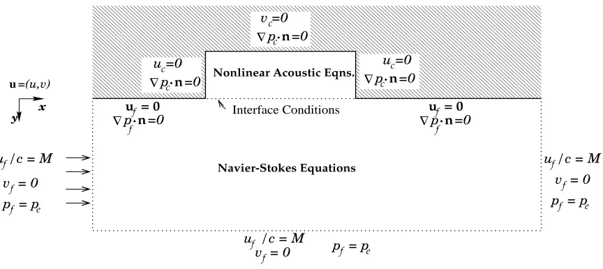
The model then consists of a set of coupled equa-tions given by

@

u

f @t

+ (

u

f r)

u

f =

0

u

f ?

rp f

0

(29)

@p f @t

=?r(p

f

u

f) (30)

p f =

c 2 0

f (31)

@ 2

u

c @t

2 ?c

2 0

u

c = ?

c

r

c

+ c 2 0

c

[(

u

c r)r

c ?(r

c r)

u

c] (32) @

c @t

=?r(

c

u

c) (33)

p c=

c 2 0

c (34)

where

u

f ;p

f ;

f are dened on f and

u

c ;p

c ;

c are

dened on c, with boundary conditions u

f

=c=M; v f = 0

p f =

p

e on ?e (35)

u

f =

0

; rp

f

n

= 0 on ?

s (36)

u

c

n

= 0; rp

c

n

= 0 on ? w (37)

wherep

eis a given pressure distribution on ?e, and

coupling conditions on ?is

v f

j y=0 =

v c

j y=0+ (

U?u c

j y=0)

@h @x ;

(38)

p f

j y=0 =

p c

j y=0

:

Here we have assumed that the articial boundary, denoted by ?e, is far enough from the cavity so that

there are no eects from uid/structure interaction.

WEAK FORM

For both theoretical and computational consid-erations it is often convenient to write a model such as that derived above in a weak or variational form. We do that here, following the general ideas used in [2] and [10].

First, we dene the framework for the uid/structure interaction model given above. Let

V

f be the subspace of

H 1(

f)

2

dened by

V f =

n 2

H

1( f)

2

: r = 0 in f

;

=

0

on ?f ??

is g;

equipped with the H

1( f)

2

-norm

k

u

k 2 V

f = k

u

k

2 [H

1 (f)]

2 = 2 X i=1

ku i

k 2 H

1 (f)

and

j

u

j 2 V

f = 2 X i=1

jru i

j 2 [L

2 (f)]

2 :

LetW

f be the subspace of H

1(

f) dened by W

f =

2H 1(

f) :

= 0 on ? e

equipped with theH 1(

f)-norm, and let V

c be the

subspace of H

1( c)

2

dened by

V c =

n 2

H

1( c)

2

:

n

= 0 on ? w

o ;

equipped with the H

1( c)

2

-norm. Let 2V

f

; 2W f

; 2V c and

2H 1(

c)

and consider the variational form of the system (29)-(34) with

u

f

2V f,

p f and

f

2W f,

u

c

2V c and p

c ;

c 2H

2( c).

We will seek solutions that satisfy homogeneous boundary conditions since these can be translated into solutions satisfying (35) in a straight forward manner (see [2]).

We then have, along with the coupling equations (38), the system

f)

;) = 0 (40)

(p f

;)?c 2 0(

f

;) = 0 (41)

@ 2

u

c @t

2 ;

+

@ @t

[(

u

c r)

u

c] ;

(8)

?c 2 0 ?

u

c ;

+

c

2 0

r c

c

u

c r

c

c ;

?

c 2 0

c

[(

u

c r)r

c ?(r

c r)

u

c] ;

?2c 2 0

r

u

c

r c

c ;

= 0 (42)

@

c @t

;

+? r(

c

u

c) ;

= 0 (43)

? p

c ;

?c

2 0 ?

c

;

= 0; (44)

where ~S is dened by

~

S?p f

I+r

u

f

:

Remark 11

Recall that for constant the

diver-gence of the stress tensor, given by

r S f =

r n

?p f

I+ h

r

u

f+ (

u

f) T

io ;

reduces to

r S f =

r(?p f

I+r

u

f)

:

(see Remark 1). Thus, we have

rS f =

rS:~

We note that

((

u

r)

v

;

1( f)

2

, combined with Green's formula

(r ;)

f = (

n

;)

@ f

?( ;r)

f

; (47)

where 2

H 1(

f)

2

; 2 H 1(

f). The

r)v

2 ;w

n

u

;w

2)? f

= ?(

v

(r

w

) T

;

u

) + (

vn

u

;

w

) ?

is ;

where we recall thatr

u

= 0 in

f and

w

=

0

on

?f ??

is.

Again using Green's formula and introducing the coecient of kinematic viscosity denoted by = =

0, we see that the equation (39) becomes

@

u

f @t

n

; ) ?is= 0

:(48)

Remark 12

Note that in the above computation we assumed

S=~ 0

;

?is

?(

n

p f

= 0

; ) ?is

:

Remark 13

In the equation(48) we have used the fact that the outward normal vector to?isis pointing

upward, away formf, and because of the coordinate

system chosen, we have

u

f

n

=?v f

:

Consider now the equation (42) given by

@

2

u

c @t

2 ;

+

c r

c

c ;

?

c 2 0

c

[(

u

c r)r

c ?(r

c r)

u

c] ;

?2c 2 0

r

u

c

r c

c ;

= 0:

The second term on the left side can be written as

@ @t

[(

u

c r)

u

c] ;

=

@

u

c @t

r

u

c ;

+

(

u

c r)

@

u

c @t

;

:(49)

) T

;

u

)?(

v

r

u

;

w

)

+(

v n

u

;

w

) ?

is

(9)

Applying this identity to each term on the right side of (49), we nd

@ @t

c @t

n

u

c ; ?is =?

u

c ? r T ; @

u

c) ; ?is :

u

c r)r

c ?(r

c r)

u

c] ;

= 0: (51)

Therefore, by using equations (48) and (51) and (38), the variational formulation for the system (29)-(34) may be written as the coupling equation (38) along with the equations

@

u

f @t ;

+a(

u

f

; )?b 1(

u

v f

;) ?

is = 0(53) ? p f ?c 2 0 f ;

= 0 (54)

@ 2

u

c @t 2 ; +c 2 0

a(

u

c ; ) ? b 1

u

c ; ; @

u

c @t +b 1 @

u

c @t

c ; r c c ; ? 2c

u

c v c) ; ?is = 0 (55) @ c @t ;

?e(

u

c

; c

;) + (v c

c

;) ?

is = 0 (56) ? p c ?c 2 0 c ;

= 0; (57)

where the forms a(;), b 1(

;;), e(;), a( ;), b

1(

;;), b 11(

;;), b 2(

;;), b 3(

;;), d( ;) and e(;;) are dened as follows

a(

) T

;

w

); b

11(

u

;

v

;

w

) = (r

u

v

;

w

); b

); b

v

)

2V cand

r;q2 H

1( c).

REFERENCES

[1] G.K. Batchelor, An Introduction to Fluid Dy-namics, Cambridge University Press, 1967.

[2] H.T. Banks and K. Ito, \Structural Actuator Control of Fluid/Structure Interactions," Proc. 33rd

Conference on Decision and Control, Lake Buena Vista, Fl, Dec. 1994, pp.283-288.

(10)

[4] A.J. Chorin and J.E. Marsden, A Mathe-matical Introduction to Fluid Mechanics, Springer-Verlag, NY, 1990.

[5] P.G. Drazin and W.H. Reid, Hydrodynamic Stability, Cambridge University Press, 1981. [6] H.H. Heller and D.B. Bliss, \Flow-Induced Pressure Fluctuations in Cavities and Concepts for their Suppression," AIAA 2ndAero-Acoustics

Con-ference, Hampton, VA, March 1975, Paper 75-491. [7] D.Y. Hsieh and S.P. Ho, Wave and Stability in Fluids, World Scientic Pub., Singapore, 1994. [8] D. Rockwell and E. Naudascher, \Review{ Self-Sustaining Oscillations of Flow Past Cavities," Journal of Fluids Engineering, Vol. 100, June 1978, pp.152-165.

[9] R.L. Sarno and M.E. Franke, \Suppression of Flow-Induced Pressure Oscillations in Cavities," Journal of Aircraft, Vol. 31, No. 1, Jan.-Feb. 1994, pp.90-96.

[10] R. Temam, Navier Stokes Equations: The-ory and Numerical Analysis, North-Holland, Ams-terdam, 1971.

00000000000000000000000000000000 00000000000000000000000000000000 00000000000000000000000000000000 00000000000000000000000000000000 00000000000000000000000000000000 00000000000000000000000000000000 00000000000000000000000000000000 00000000000000000000000000000000

11111111111111111111111111111111 11111111111111111111111111111111 11111111111111111111111111111111 11111111111111111111111111111111 11111111111111111111111111111111 11111111111111111111111111111111 11111111111111111111111111111111 11111111111111111111111111111111

Figure 5: Flow-Cavity Model u = 0

∆ _{p =0}_._n

u /c = M

v = 0 p = pf f

f f

f

p = p_f _e p = pf

e

e ∆ _{p =0}

n . u = 0_f

f

f v = 0

u /c = M_f

f v = 0

n .

c c

n .

c

c p =0

∆

n .

c c u =0 p =0 p =0

∆

u =0

v =0

u=(u,v)

y x

Nonlinear Acoustic Eqns.

Interface Conditions

u /c = M_f