Parameter Estimation of Viscoelastic Models in a 1-D Circulatory Network

(1)

ABSTRACT

BATTISTA, CHRISTINA. Parameter Estimation of Viscoelastic Wall Models in a One-Dimensional Circulatory Network. (Under the direction of Mette S. Olufsen and Mansoor A. Haider.)

Flow and pressure waves originate from the contraction of the heart and propagate

along deformable vessels where the waves are reflected, dampened, and dispersed within

smaller sub-networks of vessels. Wave propagation in the circulatory system has been

studied from many different angles with the most successful being from a fluid dynamics

approach. This thesis develops and applies a one-dimensional nonlinear fluid dynamics

model for pulse wave propagation in large systemic ovine arteries with the goal of

enhanc-ing the understandenhanc-ing of cardiovascular disease and potentially impactenhanc-ing diagnostic tech-niques related to systemic hypertension. Hypertension, high blood pressure, is associated

with the stiffening of large or small arteries, and by stiffening the arteries in our network,

we show the impact that each has on the pressure waveform.

The Navier-Stokes equations that govern blood flow in the large arteries are highly

de-pendent upon the parameters specified by both the in- and outflow boundary conditions

as well as the coupled arterial wall model. The most common outflow boundary condition,

the three-element Windkessel model, requires diligent estimation of parameters to

pro-duce physiologically relevant and sensible results. Simultaneously, biomechanical

proper-ties of the arterial wall change along the axial direction, resulting in stiffer arteries and less viscoelasticity with progressively smaller vessels or as diseases progress. With a change in

mechanical properties of the arterial wall, in particular viscoelasticity, various amounts of

energy are lost throughout the system. Energy loss must then be compensated for in the

downstream vasculature via means of the outflow boundary conditions. Thus the

Wind-kessel model relies not only on pressure and flow but also the wall model and its

parame-ters.

While the Windkessel model has been implemented and studied for many years, the

current approach for determining the parameters has been based on elastic wall models

where minimal amounts of energy are lost as the pulse waves propagate along the network. When incorporating viscoelastic walls where larger energy losses are evident, it is a

non-trivial task to estimate the outflow boundary condition parameters. This thesis presents

a systemic approach for determining Windkessel parameters based on vessel radius,

(2)

(3)

Parameter Estimation of Viscoelastic Wall Models in a One-Dimensional Circulatory Network

by

Christina Battista

A dissertation submitted to the Graduate Faculty of North Carolina State University

in partial fulfillment of the requirements for the Degree of

Doctor of Philosophy

Applied Mathematics

Raleigh, North Carolina

2015

APPROVED BY:

Mette S. Olufsen

Co-chair of Advisory Committee

Mansoor A. Haider

Co-chair of Advisory Committee

Brooke N. Steele Pierre Gremaud

(4)

DEDICATION

For all of my grandparents....

Thank you for being my biggest fans and always reminding me I could accomplish this.

“What children need most are the essentials that grandparents provide in abundance. They give unconditional love, kindness, patience, humor, comfort, lessons in life...and most

importantly, cookies.”

(5)

BIOGRAPHY

Christina was born in Buffalo, NY and grew up in a small suburb called Alden. Upon

grad-uating high school in 2007, she attended the Rochester Institute of Technology (RIT) in

Rochester, NY where she decided to major in Applied Mathematics. After attending George

Washington University’s Summer Program for Women in Mathematics at the end of her

sophomore year, Christina knew she didn’t want her education to end after her bachelor’s degree. She registered for the BS/MS program in Applied and Computational Mathematics at RIT and added two minors, Applied Statistics and Criminal Justice, and a concentration

in Physics.

While at RIT, she participated in numerous research projects with many professors who

helped pave the way for her love of applied mathematics (Dr. Darren Narayan, Dr. Tamas

Wiandt, and Dr. David S. Ross). She worked with Dr. David S. Ross at RIT on her master’s

research project which was entitled “Parathyroid hormone and cell signaling in bone

re-modeling.” This had been the first time Christina applied mathematics to biology-related

topics and truly embraced her inner nerd. Realizing that she loved the biology as well as the mathematics being applied to it, she decided to apply for Ph.D. programs where there were

opportunities to continue applied mathematics research with biological applications.

In February of 2011, Christina received a call with news that the Department of

Math-ematics at North Carolina State University was inviting her into their graduate program.

She moved to Raleigh that June and Mansoor Haider offered her a research assistantship

for the first semester in the 2011 schoolyear. Mansoor Haider and Mette Olufsen advised

Christina through four years of research and a successful dissertation defense in August

2015. Christina has accepted a position at The Hamner Institute for Health Sciences as a

(6)

ACKNOWLEDGEMENTS

First and foremost, I would like to express my sincere appreciation to my advisory

commit-tee: Mette S. Olufsen, Mansoor A. Haider, Brooke L. Steele, Pierre Gremaud, and Sharon

Lubkin. Thank you all for providing me with support and insightful criticism throughout

this research. A special thanks to my advisors, Mette and Mansoor, for their patience and

guidance these past four years. A finite amount of words cannot do justice to thank them for helping me grow as a researcher and letting me have a little fun along the way. Their

confidence in me never faltered, even when mine did, and they always pushed me to look

at the bigger picture. Without their help and support, I wouldn’t have made it where I am

today.

A special thanks to all the friends I made during graduate school. I was fortunate enough

to have been surrounded by so many friends from the moment I moved to North Carolina.

There are too many people to list but I am grateful for the distractions provided by sporting

events, trivia, craft nights, card games, crosswords, and geocaching.,

I am especially thankful for my officemates over the years–Nakeya Williams, Gregory Mader, Christian Olsen, Jacob Sturdy, and Reneé Brady–and to the rest of the

Cardiovas-cular Dynamics Group (#wedonothing). Thank you for not only being classmates and

col-leagues, but also friends, and for making my workspace such a fun place to be. You guys

made research tolerable on the days when I didn’t think I could do it and provided me with

enough distractions throughout the process to keep me sane. Some of my happiest and my

saddest moments in graduate school happened in our office and I’m glad to have had you

there to share them with.

Thanks to the most adorable (and supportive!) four-legged friends in the world, Tippy

and Zoë, and to the recent family addition, Gus.

Lastly, and most importantly, I want to thank my family both near and far. Graduate

school is hard enough as it is and I couldn’t imagine doing it without the support of my

family. They have been there for me every step of the way, keeping me sane via phone

calls and visits, loving me unconditionally, and standing by me through all of my tough

(7)

LIST OF TABLES

Table 2.1 Percent composition of themediaandadventitiaof three arteries at in vivoblood pressure. Values given are mean±standard deviation. Adapted and reproduced with permission from[55]. . . 14 Table 3.1 Summary of data available in literature forin vivoorex vivopressure

p, areaA, and flowq. Also specified are the species and arteries from which the data is measured. . . 24

Table 4.1 General summary of blood flow modeling in 1-D and 3-D plus those that have studied and compared results in both dimensions. . . 28 Table 4.2 Summary of wall models studied by different groups. . . 37 Table 4.3 Two linear wall models written in QLV formulation with creep

func-tionK(t)and inverse elastic response functions(e)_[_p_]_{. Note that the} creep function distinguishes between elastic and viscoelastic. . . 47

Table 5.1 WIA table showing type and direction of dominating waveforms. Cor-responding discretized WIA terminology is given in parenthesis. . . 57

Table 6.1 Summary of numerical methods implemented by references to solve 1-D fluid models. MoC: method of characteristics, FDM: finite

differ-ence method, FEM: finite element method, DG: discontinuous Galerkin. 60

Table 7.1 Average geometric and mechanical optimized parameters for the elas-tic and viscoelaselas-tic wall models. Results are presented as mean± standard deviation. For all segments,n =11,h is the wall thickness, r0is the zero-strain radius,E is the Young’s modulus, andA1andb1 are the viscoelastic relaxation parameters. Parameters noted n.d. are non dimensional. . . 76 Table 7.2 Vessel dimensions and flow distribution. For each vessel segment

shown in Figure 7.4, the table specifies length, proximal and distal unstressed radius (all in cm), as well as the distribution of flow to the vessel segment[31, 82, 146]. The total cardiac output was set at 66.9 mL/s[40]. Unstressed vessel radii were averaged from optimal values presented in Table 7.1. . . 80 Table 7.3 Model parameters. Fluid dynamics parameters were used in both the

(10)

Table 7.4 Results for each of the symmetric networks whereE h/r0is constant throughout the vasculature. The increasingR1trend observed in the single vessel and 3-vessel network changes as more generations are added. However, the trends forR2andR1/Rt remain the same for the

symmetric bifurcating networks. . . 94 Table 7.5 Parameter values and units for (7.4.4) and (7.4.5). The notation n.d.

indicates non-dimensional quantities. . . 96 Table 7.6 Results for each of the symmetric networks whereE h/r0varies based

onr0throughout the vasculature.R1now increases for all networks as viscoelastic degree (A1) is increased. However, the trends forR2 andR1/Rt remain the same for the symmetric bifurcating networks. . 98

(11)

LIST OF FIGURES

Figure 2.1 A schematic showing the parallel layout of the CVS. The only circu-latory beds in series are those between the spleen, intestines, and the liver. Red arrows indicate vessels that carry oxygenated blood, blue vessels indicate those that carry deoxygenated blood. Purple boxes represent major vascular beds where the exchange of gases occurs. Adapted and reproduced with permission from[91]. . . 5 Figure 2.2 Blood flow in the heart. Systemic venous blood enters the right atrium

(RA) through the superior (SVC) and inferior vena cava (IVC) where it then passes into the right ventricle (RV). The RV ejects blood into the pulmonary artery (PA) where it passes through the lungs and is reoxygenated before flowing through the left atrium (LA) and then filling the left ventricle (LV). From here, the blood is ejected through aorta (A) to be distributed to the major organs. Used with permis-sion from [82]. . . 7 Figure 2.3 Pressure gradients in the systemic (left) and pulmonary (right)

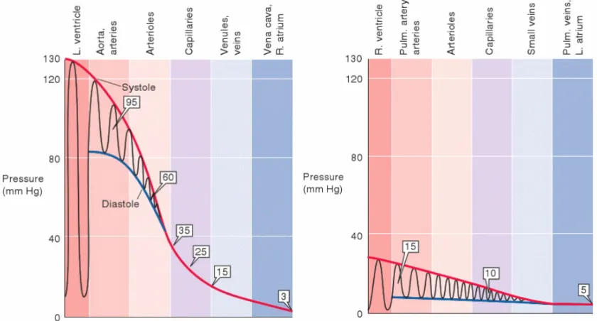
net-works, indicating that the systemic network operates at a much higher pressure than the pulmonary network. Boxed numbers mark mean pressure values at each level. Reprinted with permission from[31]. . 8 Figure 2.4 Pressure-volume loop for the left ventricle including phases of the

cardiac cycle and the opening and closing of the valves. Reprinted with permission from[91].□ . . . 9 Figure 2.5 The variation in aggregate cross-sectional area at all levels of

arboriza-tion. Aggregate cross-sectional area increases as larger arteries branch into smaller arterioles and capillaries. Adapted and reproduced with permission from[31]. . . 10 Figure 2.6 Branching of arteries and merging of veins.r indicates the typical

radius for a human at that level of arborization. Reprinted with per-mission from[31]. . . 11 Figure 2.7 Histological slices displaying a cross-section of the arterial wall from

(12)

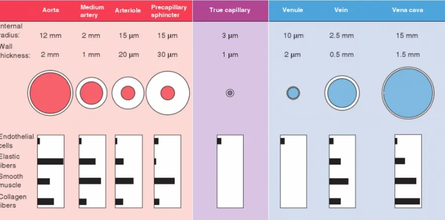
Figure 2.8 Vascular size, wall thickness, and relative composition at different levels of arborization in human vasculature. Values for medium ar-teries, arterioles, venules, and veins are illustrated. It should be noted that the dimensions vary widely vary. Wall compositions values from specific arteries are shown in Table 2.1. Reprinted with permission from[31]. . . 13 Figure 2.9 (left) A healthy pressure waveform where the forward wave

(ema-nating from the heart) occurs before the reflected wave (ema(ema-nating from the periphery). (right) As arterial walls stiffen, pulse wave ve-locity increases causing the forward and backward waves to occur at the same time, augmenting the pressure waveform. Adapted and reproduced with permission from[164]. . . 16 Figure 3.1 Mock circulation including a pneumatic pump, a perfusion line

con-nected to the chamber with the mounted vessel segment, a resis-tance modulator (R), and a reservoir. The chamber was filled with a thermally controlled Tyrode’s solution. Pressure (p) was measured with a micro transducer while the diameter (D) was measured with a pair of ultrasonic crystals using sonomicrometry. . . 20 Figure 3.2 Pressure-area, pressure time series, and area time series data from

each of the seven excised vessels. Corresponding colors represent vessels from the same sheep. From top left to bottom right: AA, BT, CA, DA, FA, MA, and PA. . . 25

Figure 4.1 The velocity profile for varying values ofγand the no-slip bound-ary condition inside a vessel with radiusr along the axial direction x. Asγincreases, the shape changes from a parabolic profile (cor-responding to a fully developed flow) to a blunt profile (mimicking a pulsatile flow). This work assumes a parabolic profile correspond-ing toγ = 2. At a solid boundary (the arterial wall wherer = R ), the blood has zero velocity relative to boundary. This is true for any timet and anyx along the axial direction. . . 32 Figure 4.2 The three simplest linear viscoelastic models composed of springs

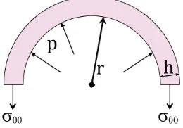
and dashpots: (a) Maxwell, (b) Voigt, and (c) Kelvin. Linear springs produce instantaneous deformations proportional to the load while dashpots slow motion, absorb energy, and produce velocity propor-tional to the load. . . 36 Figure 4.3 A diagram of the forces acting on a vessel under static equilibrium

conditions. TheFo u t w a r dis due to blood pressure acting on the

inte-rior wall of the vessel andFi n w a r d is the force acting on the exterior

(13)

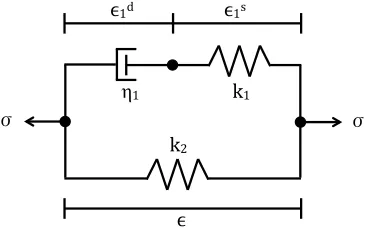
Figure 4.4 The Kelvin viscoelastic model illustrated using mechanical analogs with a combination of two Hookean elastic springs and a dashpot. . 40 Figure 4.5 The WK analogy to an air chamber. . . 50 Figure 4.6 Diagram depicting the three-element WK model. . . 51

Figure 6.1 (1st row) Maintaining the time steps per period (1200) converges for any number of elements. This shows spatial convergence for a straight elastic vessel. (2nd row) The temporal residual errors shown for pressure and area of an elastic non-tapered vessel on a log-log plot. (3rd row) The vessel is discretized spatially into 12 elements while increasing the time steps per period: 200, 400, 800,1200, 2400, 4800, 9600. It is apparent that the solutions corresponding to 800, 1200, 2400, 4800, and 9600 time steps are the same, thus signifying temporal convergence of the solver. (4th row) The spatial residual errors shown for pressure and area of an elastic non-tapered vessel on a log-log plot. . . 70 Figure 6.2 (1st row) Convergence in space for the viscoelastic wall model for

a non-tapered vessel with 1200 time steps per period. Although we change the number of elements (spatial mesh), we obtain the same results thus signifying convergence. (2nd row) The spatial residual errors shown for pressure and area of a viscoelastic non-tapered vessel on a log-log plot. (3rd row) Temporal convergence for the viscoelastic wall model with a non-tapered vessel discretized spa-tially into 12 elements. If each period is discretized into 800 or more time steps, we see convergence of the solver. (4th row) The tempo-ral residual errors shown for pressure and area of a viscoelastic non-tapered vessel on a log-log plot. . . 71 Figure 6.3 (1st row) Maintaining the time step at 800 per period, we obtain

(14)

Figure 6.4 (1st row) Convergence in space for the viscoelastic wall model in a tapered vessel. Although we change the number of elements (spa-tial mesh), we obtain the same results for 100+elements, thus signi-fying convergence. (2nd row) The spatial residual errors shown for pressure and area of a viscoelastic tapered vessel on a log-log plot. (3rd row) Temporal convergence for the viscoelastic wall model with a tapered vessel discretized spatially into 12 elements. (4th row) The temporal residual errors shown for pressure and area of a viscoelas-tic tapered vessel on a log-log plot. . . 73

Figure 7.1 Elastic modulus and zero-strain radius optimized values for larger ovine arteries. . . 77 Figure 7.2 Measured diastolic radius values plotted against the theoretical,

op-timized elastic zero-strain radius for each sheep in each vessel. . . 78 Figure 7.3 The best fit exponential decay function for all data points including

those from the sheep data and those provided in Olufsen’s disserta-tion. . . 78 Figure 7.4 The network geometry. The seven arteries from which pressure-area

measurements have been taken are marked with letters (AA, BT, CA, PD, MD, DD, FA), while other major vessels are marked with letters in parenthesis (CM, RA, IL, IT). In the model, the renal arteries and the celiac and mesenteric arteries were each combined into a sin-gle vessel, and the carotid, iliac, and femoral bifurcations were mod-eled as symmetric. . . 79 Figure 7.5 Flow and pressure-area computations and data for each vessel in

the network. . . 83 Figure 7.6 Pressure and flow waveforms along the aorta in an elastic network.

Systolic pressure increases progressing toward the periphery. . . 84 Figure 7.7 Single non-tapered vessel representative of the ascending aorta where

we have assumed a non-tapering vessel. This geometry is used to study the affects of the in- and outflow boundary conditions. . . 84 Figure 7.8 Model predictions in a single vessel (the ascending aorta)

mimick-ing results from a specific sheep. . . 85 Figure 7.9 Effect of changing the WK parameters in a single vessel network. . . . 87 Figure 7.10 Effect of changing the compliance parameter values in a single

ves-sel network. . . 88 Figure 7.11 Effect of changing wall viscosity while keeping outflow boundary

(15)

Figure 7.12 (Top) Results for matching pulse pressure in a single vessel. By in-creasing the peripheral resistance in the WK model as wall viscoelas-ticity increases, we are able to obtain the same pulse pressure but mean pressure increases. (Bottom) Results for matching mean pres-sure in a single vessel. As wall viscoelasticity increases, the distal re-sistance in the WK model must decrease in order to maintain the same mean pressure. However, this simultaneously leads to an in-crease in pulse pressure. . . 89 Figure 7.13 Increasing wall viscoelasticity while maintaining constant pulse and

mean pressures requires an increase in proximal resistance and a decrease in distal resistance of the WK model, conserving the to-tal resistance. TheR1/RT ratio, previously taken to be 0.2[99], is

di-rectly correlated with wall viscoelasticity. As seen in the left bottom row, matching pulse pressure and mean pressure maintains pres-sure shape and size. . . 90 Figure 7.14 Symmetric geometries used to determine WK parameters in

viscoelas-tic networks. From left to right: 3-, 7-, and 15-vessel networks. Note that these are representative and do not reflect the actual geometries. 91 Figure 7.15 R1andR2associated with each daughter vessel plotted as functions

ofςandA1. The total network resistance is defined as 2RTd where

RTd =R1+R2as shown in the figures. Red lines show the functions

given by (7.4.1) and (7.4.2). . . 92 Figure 7.16 A circuit of resistorsR1,R2, . . . ,Rn in parallel. The total resistance of

the circuit can be calculated using (7.4.3). . . 93 Figure 7.17 Total resistance in each symmetric network for increasing values

ofA1. It is important to note that whenA1=0, corresponding to a purely elastic wall, the networks have the same total resistance. This supports our hypothesis that as viscoelastic vessels are added into a network, more energy is lost and thus higher resistances are needed at the outflow boundary conditions to account for these losses. The total resistance corresponding to the elastic models matches the to-tal resistance found in the single vessel network and is equal to the mean pressure divided by the mean flow (RT =p¯/q¯). . . 95

(16)

Figure 7.19 Total resistance in each symmetric network for increasing values of A1. Again, the total resistance remains the same in each network for the elastic wall model and can be found viaRT =p¯/q¯. As more

vis-coelastic vessels are added to the network, higher resistances are needed in the WK models to account for energy losses due to the wall model. . . 99 Figure 7.20 R1(left) andR2(right) as functions ofA1and r0 for symmetric

net-works where E h/r0 is the same in all vessels. Both R1 and R2 are defined as second-order polynomials inA1andr0. . . 100 Figure 7.21 WIA in a single straight vessel whereE h/r0 is varied with an

elas-tic wall (top) and whereA1is varied in the viscoelastic model (bot-tom). The normal E h/r0 value is shown in black. E h/r0 varies as 25%, 50%, 150%, and 200% of this value.A1varies between 0 and 0.8 in increments of 0.2. . . 102 Figure 7.22 WIA for 3-vessel networks: (top)E h/r0 constant, (bottom) E h/r0

varying withr0. A1 =0 corresponding to the elastic case is shown in red; increasingA1given by the spectrum order. Velocity appears similar in the two cases; this is different from Figures 7.23 and 7.24. . 103 Figure 7.23 WIA for 7-vessel networks: (top)E h/r0 constant, (bottom) E h/r0

varying withr0. In the case ofE h/r0varying exponentially withr0, the pressure and velocity waveforms are lined up for all cases of vis-coelasticity validating our method for choosing WK parameters. . . . 104 Figure 7.24 WIA for 15-vessel networks: (top)E h/r0constant, (bottom)E h/r0

varying with r0. The pressure and velocity waveforms are lined up for all cases of viscoelasticity whenE h/r0varies exponentially with r0. . . 105 Figure 7.25 WIA in the ascending aorta from an elastic network mimicking healthy

(17)

Chapter 1 Introduction

Cardiovascular diseases, defined as disorders of the heart and blood vessels, are the

num-ber one cause of death globally with 17.5 million deaths in 2012[181]and an estimated 23.6 million deaths in 2030. One of the major risk factors for cardiovascular disease is

hy-pertension, or elevated blood pressure. Hypertension can lead to coronary heart disease

and is considered the most important risk factor for stroke, causing more than half of

is-chaemic strokes (obstruction of blood to the brain) and drastically increasing the risk for hemorrhagic stroke (ruptured vessels that bleed into the brain)[181].

One-third of the adult population (70 million people) in the United States suffers from

hypertension and only half have their condition under control[36]. Another 70 million adults are prehypertensive[36], indicating a risk for hypertension. The etiology of hyper-tension is largely unknown[18], with little to no progress towards achieving an accepted hypothesis. The past century provided hypotheses on the relationship between

hyperten-sion and arteriosclerosis, and suggested that the splanchnic nerves and circulation play

major roles in hypertension. One hypothesis is that the pathophysiology associated with

the stiffening of large or small arteries causes changes in the hemodynamics and wave propagation in the circulatory network. Novel hypotheses on the etiology of hypertension,

such as stiffening of arteries, can be interpreted and supported (or rejected) via means of

(18)

1.1 Summary of the dissertation

My work focused on 4 aims: (1) to derive a 1-D fluid dynamics model that can be

cou-pled with elastic or viscoelastic arterial wall models to study wave propagation, (2) to es-timate parameters associated with arterial wall models and determine how these change

with arterial cross-sectional area, (3) to construct and validate a systemic ovine arterial

network model predictingex vivopressure and area, and (4) to develop a systematic

ap-proach analyzing how energy losses due to wall viscoelasticity effect outflow boundary

conditions. The latter is important for network simulations which require large

computa-tions with many parameters, all of which must be estimated to obtain physiological results.

Elastic networks are easier to calibrate than viscoelastic network. By forming a systematic

approach to estimating outflow parameters in viscoelastic arteries, network simulation

construction is simplified.

• Chapter 2 introduces structural and functional properties of the cardiovascular

sys-tem relevant for the models developed in Chapter 4.

• Chapter 3 describes the experimental procedures used by the Hemodynamics

Lab-oratory at the Universidad de la República in Montevideo, Uruguay to acquire

pres-sure and area data from systemic ovine arteries. Moreover, it provides an overview

of literature data available for validating 1-D blood flow models.

• Chapter 4 derives the 1-D model used for predicting arterial blood pressure,

volu-metric flow, and cross-sectional area in arterial networks. The major components are a 1-D fluids model, arterial wall models, and models of the boundary conditions.

The 1-D fluids model is derived from the Navier-Stokes equations under the

assump-tion of an axisymmetric, incompressible flow. The arterial wall models use the

frame-work of Fung’s quasilinear viscoelasticity theory which formulates arterial strain as a

function of stress. The outflow boundary conditions are modeled by a three-element

Windkessel model, relating pressure and flow at the outlet of terminal vessels. Each

of these three components are accompanied by a literature review.

• Chapter 5 briefly presents wave intensity analysis, a method for analyzing wave

(19)

• Chapter 6 sets up the numerical scheme used to solve the system of partial

differen-tial equations. A stabilized space-time finite element method based on a

discontinu-ous Galerkin method in time was utilized to solve the nonlinear equations governing

pulsatile blood flow in the arteries. Results confirming convergence of the solver in

a single vessel geometry are shown.

• Chapter 7 shows results for computations with elastic and viscoelastic networks. The

inverse problem allowing for estimation of wall model parameters is briefly described.

An elastic network geometry is developed and used to confirm the adequacy in using

discreteex vivodata in network simulations. The viscoelastic network is the heart of this dissertation and builds upon smaller networks to construct a clearcut way to

pre-dict outflow boundary conditions based on geometry, wall viscoelasticity, and vessel

stiffness.

• Chapter 8 summarizes the key points addressed in this dissertation and suggests

(20)

Chapter 2 Cardiovascular Physiology

This chapter presents the cardiovascular system, specifically the systemic arterial network

which distributes blood from the left ventricle to the periphery. The general information

presented here is from physiology books by Boron [31], Smith and Kampine[146], Lev-ick[91], and Klabunde[82]. Section 2.1 outlines the cardiovascular system (CVS) and its functions while Section 2.2 presents various properties of the vasculature as well as

com-mon diseases affecting the arterial wall.

2.1 The cardiovascular system

The CVS is composed of a sophisticated network of blood vessels that facilitates the

trans-portation of nutrients (oxygen, glucose, amino acids, fatty acids, vitamins, drugs, water) to

and the removal of metabolic waste products (carbon dioxide, urea, creatinine) from

tis-sues. There are three primary components of the CVS: 1) a pump (the heart), 2) the liquid

(blood), and 3) a network (vessels). The system consists of two main divisions that form a

(21)

HEAD & ARMS

LUNGS

LIVER

STOMACH & INTESTINES

KIDNEYS

LOWER BODY & LEGS

Pulmonary

vein Pulmonary

artery

Aorta

Heart

Hepatic artery Hepatic vein

Hepatic portal vein Inferior

vena cava Superior vena cava

Renal vein Renal artery

Figure 2.1A schematic showing the parallel layout of the CVS. The only circulatory beds in series

are those between the spleen, intestines, and the liver. Red arrows indicate vessels that carry oxy-genated blood, blue vessels indicate those that carry deoxyoxy-genated blood. Purple boxes represent major vascular beds where the exchange of gases occurs. Adapted and reproduced with permis-sion from[91].

2.1.1 The systemic and pulmonary circuits

The heart, weighing only 300 grams, contains four chambers (Figure 2.2), making up two

pumps that feed the pulmonary and systemic circulatory[146]. The pulmonary circuit in-volves the flow of deoxygenated blood from the right heart to the lungs, the flow within the

lungs, and the flow of oxygen-rich blood back to the left heart. As blood passes through

the lungs, oxygen and carbon dioxide are exchanged between the capillaries and the gases

within the alveoli. The oxygenated blood is transported from the left heart throughout the

body via thesystemic circulationto organs where it diffuses from the blood into the

(22)

the tissues into the blood where they are transported back to the lungs and the exchange

between blood and gases is made once again. Compared to the pulmonary circuit, the

systemic circuit operates under a higher mean pressure as shown in Figure 2.3, 15 and 95

mmHg, respectively[31].

The right and left sides of the heart each contain an atrium and a ventricle. The left

ven-tricle and left atrium are connected via the mitral (or bicuspid) valve which, under normal

conditions, prevents back flow from the ventricle into the atrium. The right ventricle and

right atrium are connected via the tricuspid valve which serves a similar purpose as the

mitral valve. Venous blood from the systemic circulatory system is returned to the heart through the right atrium, and the right ventricle then cycles the blood to the pulmonary

circuit. The blood leaves the pulmonary system and enters the left atrium via pulmonary

veins where it then flows into the left ventricle. The left ventricle ejects blood into the

sys-temic circuit, beginning with the aorta which then, in turn, distributes the blood

through-out the body to all the organs. Blood that flows from the aorta to the major organ systems

ultimately enters the venous system, the superior and inferior vena cava, and is then

re-turned to the heart. Circulation to the major organ systems occurs primarily in parallel as

shown in Figure 2.1.

Within organs, the arterial vasculature branches into smaller and smaller vessels. This branching, along with the decrease in radial size of the arteries, is vital to maintaining

blood pressure and flow throughout the network. Its importance will be emphasized in

the next section.

2.1.2 The circulation of blood

The walls of the heart are composed of muscle tissue called the myocardium. The

my-ocardium consists of three layers: the two outermost layers of fibers are diagonally

ori-ented from the base of the heart to the apex, and the innermost layer is circumferentially

oriented. Upon contraction, the innermost layers shorten the ventricular wall, pulling the

apex towards the base while the circumferential fibers constrict the ventricular diameter

of the heart.

As the heart pumps blood into the vasculature, a pressure gradient is induced within the network. This can be described by classical hydrodynamic laws, the most important in

this scenario analogous to Ohm’s law of electricity. Thus, the pressure difference (∆P)

(23)

Figure 2.2Blood flow in the heart. Systemic venous blood enters the right atrium (RA) through the superior (SVC) and inferior vena cava (IVC) where it then passes into the right ventricle (RV). The RV ejects blood into the pulmonary artery (PA) where it passes through the lungs and is re-oxygenated before flowing through the left atrium (LA) and then filling the left ventricle (LV). From here, the blood is ejected through aorta (A) to be distributed to the major organs. Used with permission from [82].

pressure gradient is required to drive a given flow through a vessel with higher resistance:

∆P =Q R. (2.1.1)

Alternatively, arterial resistance can be calculated based on vessel lengthLand radius

r if the flow fulfills Poiseuille’s law i.e. a fully-developed flow of a viscous liquid through a rigid, cylindrical pipe where the flow velocity varies from zero at the walls to a maximum

along the centerline. Where applicable, this resistance is given as

R= 8

π ηL

r4 (2.1.2)

whereηis the viscosity. Based on Poiseuille’s law, in wide vessels (such as the aorta),

re-sistance is low because there is a larger area for the flow to pass through. In contrast, the

resistance is higher in narrower vessels. In humans, large arteries account for 2% of the

total systemic resistance, whereas the arterioles, capillaries, and the venous system make

up 60%, 20%, and 15%, respectively[31].

The cardiac output (CO) is defined as the amount of blood ejected during each

(24)

Figure 2.3Pressure gradients in the systemic (left) and pulmonary (right) networks, indicat-ing that the systemic network operates at a much higher pressure than the pulmonary network. Boxed numbers mark mean pressure values at each level. Reprinted with permission from[31].

CO=SV·HR, (2.1.3)

i.e. changes in the heart rate or stroke volume will influence the cardiac output. The heart rate is determined by groups of cells known as pacemaker cells. These cells generate action

potentials that are conducted throughout the heart and trigger contraction of the cardiac

myocytes (or cardiac muscle cells.) This contraction results in the ejection of blood and

the force of this contraction regulates stroke volume. The magnitude of this force is

con-trolled by autonomic nerves and hormones. Stroke volume in a resting adult is typically

70-80 mL and heart rate is 60-75 beats per minute (bpm), resulting in a cardiac output

of 5L/min[146]. It can increase in response to external factors (fear, excitement) or an in-creased peripheral oxygen demand (exercise). Cardiac output has been known to increase

up to five times the normal amount during strenuous exercise[146]! At rest in the supine position, the average blood pressure is about 120/80. This corresponds to the ejection of blood in intermittent patterns during systole and rest during diastole where the systemic

(25)

The systolic and diastolic portions allow the cardiac cycle to divide into an active phase

and a relaxed phase (see Figure 2.4). The active phase results in an increase in pressure

while the volume remains constant. When the ventricular pressure exceeds the arterial

pressure, the aortic valve opens (initiating systole) and blood flows into the aorta. Systole

ends when the aortic valve closes and ventricular pressure drops below the arterial

pres-sure. The mitral valve opens and blood passes from the atrium into the ventricle. The mitral

valve closes, initiating the cycle again.

Figure 2.4Pressure-volume loop for the left ventricle including phases of the cardiac cycle and

the opening and closing of the valves. Reprinted with permission from[91].□

2.1.3 Vasculature

The aorta, stemming from the heart, is the largest artery in the body and branches into many large conduit arteries. These arteries branch repeatedly into smaller arteries which

branch into even smaller vessels called arterioles, known to have a very high resistance.

Ar-terioles ultimately branch into an abundant number of thin-walled capillaries 2.6. Through

arborization, or branching of the arterial network, the number of vessels increases thus in-creasing the aggregate cross-sectional area at each level (Figure 2.5).

(26)

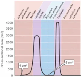
Figure 2.5The variation in aggregate cross-sectional area at all levels of arborization. Aggregate

cross-sectional area increases as larger arteries branch into smaller arterioles and capillaries. Adapted and reproduced with permission from[31].

arteries,∼107_{arterioles, and}_∼₄_×₁₀10_{capillaries (radii}_∼₃_µ_{m.) These capillaries then} con-verge to form venules. Venules concon-verge into small veins, ultimately merging to become

larger, named veins such as the vena cava.

The structural branching is crucial in slowing the blood flow as the vessels decrease in

size, thus increasing in vascular resistance. From (2.1.1), as resistance increases, blood flow

decreases causing the blood velocity in capillaries to be 1/200th of the arterial velocity[31]. The slowing is necessary to give the red blood cells sufficient time to exchange carbon

dioxide and oxygen. Capillaries are closest in proximity to cells in the body, and thus they

permit this exchange. Similarly, the arborized structure allows for lower blood pressure

values as vessels decrease in size. The largest drop in pressure is believed to occur in the

arterioles (as shown in Figure 2.3). For this reason, arterioles are theoretically referred to

as the resistance vessels although pressure in these vessels cannot be measured but rather

shown computationally[126].

(27)

act-Figure 2.6Branching of arteries and merging of veins.r indicates the typical radius for a human at that level of arborization. Reprinted with permission from[31].

ing as blood reservoirs, are referred to as capacitance vessels. Venules and small veins

outnumber their counterparts (arterioles and arteries)[29], consequently their aggregate cross-sectional area is high and aggregate resistance is low. Thus, a smaller pressure drop

of 10–15 mmHg is sufficient to drive the cardiac output through the venules (Figure 2.6).

At any given time, veins and venules contain about two-thirds of the circulating blood due

to their abundance and size[31].

At all levels of arborization, blood vessels contract and dilate to regulate blood pressure,

control blood flow within organs, and distribute blood volume throughout the body. The

arterial wall alters in response to the activation of vascular smooth muscle within the wall

by autonomic nerves, metabolic and biochemical signals outside the artery, and

vasoac-tive substances released by cells that line the artery. The wall also plays a role in producing several necessary substances (nitric oxide, endothelin-1, and prostacyclin) that regulate

the CVS functions, hemostasis, and inflammatory responses. More information on the

syn-thesis and the functions of these substances can be found in[163]and[102], respectively.

2.2 Wall tissue

All blood vessels except capillaries have walls composed of three layers–thetunica intima

(28)

It is possible to distinguish each of these layers macroscopically, as shown in Figure 2.7.

Each layer is composed of particular cells serving different roles in the mechanical

work-ings of the arterial wall. The proportion of these three layers varies depending on the size

and location of the vessel as shown in Figure 2.8 and quantified in Table 2.1.

Figure 2.7Histological slices displaying a cross-section of the arterial wall from the ovine

tho-racic aorta (left) and the carotid artery (right). The vessels were stained with orcein which allows for differentiating the three main biomechanical components of the arterial wall: elastin (dark red), collagen (blue), and smooth muscle cells (yellow). The thoracic aorta has more elastin while the carotid artery contains more collagen. The difference in these compositions explains why the wall of the carotid artery appears “stiffer” than that of the thoracic aorta. Images made available by Dr. Daniel Bia, Universidad de la República, Uruguay.[26, 159]

The innermost layer, the tunica intima, is composed of a single layer of endothelial

cells, a thin basal lamina, and a subendothelial layer. The subendothelial layer is

com-posed of collagen, smooth muscle cells, and fibroblasts. This layer serves as the barrier

that prevents plasma from seeping through the vessel wall. It also secretes many

vasoac-tive chemicals including nitric oxide which is an antithrombotic vasodilator.

Thetunica mediais primarily composed of smooth muscle cells, arranged

circumfer-entially and provides the mechanical strength and contractile power for the vessel. Elastin

(in the form of fenestrated elastic lamellae) and collagen fibers are found in this layer of arterial walls. In humans, the number of elastic lamellae is related to the anatomical

lo-cation of the artery. Muscular arteries have one internal and one external elastic lamella

(29)

Figure 2.8Vascular size, wall thickness, and relative composition at different levels of arboriza-tion in human vasculature. Values for medium arteries, arterioles, venules, and veins are illus-trated. It should be noted that the dimensions vary widely vary. Wall compositions values from specific arteries are shown in Table 2.1. Reprinted with permission from[31].

decreases toward the distal end of each arterial segment.

The tunica adventitia, the outermost layer of the arterial wall, is composed of dense

fibroelastic tissue and has no distinct outer boundary. These fibers are responsible for

releasing the vasoconstrictor agent, norepinephrin, which regulates local resistance and

therefore local blood flow. In larger arteries and veins, theadventitiaalso containsvasa

vasorum(or small blood vessels) which nourish themedia.

2.2.1 Biomechanics of wall tissue

Arterial walls exhibit both passive and active deformation. Passive components, namely

elastin and collagen fibers found in thetunica media, determine the elastic, viscous, and

inertial properties exhibited by the wall. The smooth muscle contraction during

vasocon-striction is theactive componentof the arterial wall.

Elastin, considered to be the primary determinant in blood flow dynamics, is six times more extensible than rubber, and it enables large arteries to serve as temporary blood

(30)

Table 2.1Percent composition of themediaandadventitiaof three arteries atin vivoblood pres-sure. Values given are mean±standard deviation. Adapted and reproduced with permission from[55].

Thoracic aorta Pulmonary artery Plantar artery Media

Smooth muscle 33±10 46±8 61±7

Ground substance 6±7 18±9 26±6

Elastin 24±8 9±3 1±1

Collagen 37±10 27±13 12±8

Adventitia

Collagen 78±14 63±9 64±10

Ground substance 11±10 25±8 25±9

Fibroblasts 9±11 10±6 11±3

Elastin 2±3 2±2 0±0

to accommodate the blood ejected from each heartbeat. Stretched elastin stores

mechani-cal energy which is used during diastole to maintain blood pressure and drive flow through

the downstream resistive vessels. This mechanical energy allows blood pressure to stay

above∼80 mmHg despite the fact that the heart ejects blood intermittently with the least amount of energy expended.

Collagen, whose fibers are ∼100 times less distensible than elastin, stretches only 3 to 4% under physiological conditions. It prevents vessels from excessive expansion when

blood pressure rises.

While elastin breaks down with age, collagen is built up and dominates the elastic

prop-erties of the vessels. Vessels get stiffer in a process called arteriosclerosis. This is part of the natural aging process, but vessels can also stiffen earlier and at quicker rates with the

pres-ence of cardiovascular diseases such as hypertension and diabetes[44].

Although all wall components contribute to viscosity, the magnitude of internal

fric-tion, smooth muscle cells in thetunica intimaandmediarespond to physiological stimuli.

Smooth muscle tone depends on blood flow, blood viscosity, and hematocrit values.

Char-acterizing the viscous behavior of arterial walls sheds light on the physiological factors

associated with plaque build-up or other arterial disease stages.

Due to the wall viscosity controlled by elastin, collagen, and smooth muscle cells, a

(31)

caused by the energy required to dilate a vessel during systole that is not recovered during

diastole. It is common to plot and compare these loops at various locations in the body. By

plotting hysteresis loops along a network, it is clear that vessels display different degrees

of viscoelasticity. Wall viscosity varies depending on the state of the wall muscle and other

arterial properties[26].

2.2.2 Vascular pathology

As discussed by Humphrey[74], the leading causes of morbidity and mortality are diseases of and injuries to the arterial vasculature. We will briefly outline the biomechanics of two

common pathologies but refer the reader to[74]for further information.

2.2.2.1 Hypertension

Hypertension is defined as an elevation in blood pressure from the normal 120 mmHg/80 mmHg. There are multiple criteria used to distinguish what constitutes an “above average”

or “high” pressure[129]. In humans, systemic hypertension is typically characterized by systolic pressures greater than 160 mmHg or diastolic pressures greater than 90 mmHg.

Many clinicians now diagnose “pre-hypertension” which is thought to be a intermediate

stage between normal and hypertensive patients. Pre-hypertensive patients have a systolic

pressure between 121–159 mmHg or a diastolic pressure between 81-90 mmHg and are at risk of becoming hypertensive.

The etiology of hypertension remains unknown[18], but accepted causes include ag-ing, genetics, improper diet, and malfunction of major organs or nervous systems. When

hypertension clearly results from another condition or disease, it is referred to assecondary

hypertension. In opposition, when the cause is not due to another disease and is suspected to stem from vessel stiffening, it is referred to asprimary hypertension.

As previously mentioned, within themedia, elastin deteriorates with age and collagen

becomes the dominating biomechanical substance in the arterial wall. This leads to an

increase in stiffening which causes blood flow velocity to increase and reflected waves oc-cur in sync with forward propagating waves (see Figure 2.9). This results in an augmented

pressure waveform, a symptom of arterial hypertension. Hypertension is inevitable as

hu-mans age due to the deterioration of elastin. However, in other cases of hypertension, it is

(32)

Figure 2.9(left) A healthy pressure waveform where the forward wave (emanating from the heart) occurs before the reflected wave (emanating from the periphery). (right) As arterial walls stiffen, pulse wave velocity increases causing the forward and backward waves to occur at the same time, augmenting the pressure waveform. Adapted and reproduced with permission from[164].

2.2.2.2 Arteriosclerosis

While hypertension mainly affects themedia, arteriosclerosis is a local disease of the

in-tima and the most common vascular disease overall. arteriosclerosis affects large- and medium-sized arteries, causing heart disease, stroke, and gangrene in the extremities via

fatty deposits along the inner lining of the arterial wall. This affects the structure and

func-tion of blood vessels.

It has been suggested that following an insult to the endothelium and smooth muscle of the arterial wall, monocytes adhere to the local insult and migrate to the inner wall. There,

they transform into macrophages and ultimately lipid foam cells. Meanwhile, smooth

mus-cle cells are stimulated to migrate into theintimawhile calcium is accumulated locally.

Between the two mechanisms aforementioned, the fatty deposits are locally deposited,

typically at sites of complex geometry, and prevent normal blood flow to the downstream

vasculature. This impairs the delivery of oxygen to tissues and impacts bodily function.

2.2.2.3 Relevant pathology

Because this dissertation focuses on one-dimensional modeling of blood flow in the

ar-teries, we must remain realistic in the capabilities of our model. There are particular

dis-eases which can be addressed while utilizing a one-dimensional network and those which

(33)

based on the uncertainty associated with causes for arterial hypertension. That said, this

research mainly investigates healthy arterial networks in hopes that this will lead to

im-provement of tracking diseases and understanding the structural changes in vasculature

(34)

Chapter 3 Experimental Data

The experimental data used throughout this thesis were provided by Dr. Daniel Bia and

his laboratory in the Physiology Department at the Universidad de la República in

Monte-video, Uruguay and have been used by Valdez-Jasso et al.[159–162]to develop constitutive equations relating blood pressure and arterial cross-sectional area. As discussed in

Sec-tion 3.1 and shown in SecSec-tion 3.2, data recorded are time series measurements of arterial

blood pressure and vessel diameter in ovine arteries. Measurements are taken from seven vessels in the systemic arterial network underex vivoexperimental conditions in eleven

male Merino sheep. Section 3.3 details the literature data.

3.1 Experimental setup

3.1.1 Surgical preparation and acquisition of segments

Details on the experiment are summarized from[26]. Blood pressure and cross-sectional area were measured in vessels excised from eleven healthy male Merino sheep, aged

18-24 months with a mean weight of 32 kg (ranging from 25-35 kg). All protocols were

ap-proved by the Research and Development Council of the Universidad de la República and

were conducted in accordance with the guidelines for the care and use of laboratory

(35)

ad-ministration of pentobarbital (35 mg/kg). Alveolar ventilation was maintained by a respi-rator (Draeger SIMV Polyred 201, Madrid, Spain). Respirespi-ratory rate, tidal volume, and the

inspired oxygen fraction were adjusted to maintain arterialpCO2 at 35-45 millimeters of

mercury (mmHg), pH at 7.35-7.4, andpO2 above 80 mmHg. In each sheep, seven arteries

(see Figure 7.4) were selected to evaluate their mechanical properties: the right carotid

artery (CA), the brachiocephalic trunk (BT), the ascending aorta (AA), the proximal

de-scending aorta (PD), the medial dede-scending aorta (MD), the distal dede-scending aorta (DD),

and the left femoral artery (FA). For each vessel, a 6 cm segment (marked with suture

refer-ences in the adventitia) was dissected from the surrounding tissue. Two miniature piezo-electric crystal transducers (5 MHz, 2mm in diameter) were sutured in the adventitia on

opposite sides of each vessel, and the external vessel diameter was measured by

convert-ing the transit time of the ultrasonic signal (1580 m/s) between the crystals into distance by means of a sonomicrometer (1000 Hz frequency response, Triton Technology, Inc., San

Diego, CA). Optimal positioning of the dimensionless gauges was assessed with an

oscil-loscope (model 465B, Tektronix, Richardson, TX). After marking the vessel segments, the

animals were sacrificed with an intravenous overdose of pentobarbital followed by

potas-sium chloride, and the arterial segments were excised. To limit rupture of the adventitia

and endothelium, the “no-touch” technique was employed to excise and mount (in a mock circulation) the arterial segments. After completion of the excision, the correct position of

the ultrasonic crystals as well as strength and adequacy of the suture were confirmed by

visual inspection.

In summary, six steps were performed prior to theex vivomechanical tests[11]: 1) an-imals were anesthetized; 2) seven arterial segments were exposed and dissected from the

surrounding tissue in each animal; 3) each arterial segment was marked with two suture

references in the adventitia; 4) a pair of ultrasonic crystals was sutured into the adventitia

to measure the external diameter; 5) the animals were sacrificed; and 6) the segments were

excised.

3.1.2 Ex vivo

experiments

As shown in Figure 3.1, the excised vessel segments were non-traumatically mounted in the organ chamber of the mock circulation, immersed and perfused with a thermally

regu-lated (37◦C) and oxygenated Tyrode’s solution with pH 7.4. The mock circulation consisted

(36)

Salt Lake City, UT). The pneumatic device was regulated via an air supply machine that

allowed adjustments of hemodynamic parameter values and waveforms. The external

ar-terial diameter was measured using sonomicrometry, employing the ultrasonic crystals

sutured into the adventitia during thein vivoprocedures. Pressure was measured with a

solid-state microtransducer (Model P2.5, 1200 Hz frequency response, Konigsberg

Instru-ments, Inc., Pasadena, CA) inserted into each artery through a small incision. This

tech-nique allows adequate and reproducible measurements of the arterial wall mechanics [10]. Pressure sensors were calibrated using a mercury manometer. To avoid signal interference,

the pressure sensor was inserted 2 mm proximal to the ultrasonic crystals. Experimental pressure-area data are summarized in Figure 7.5 depicting pressure area loops for each

vessel segment. These measurements are obtained by setting the inflow as mimicking the

cardiac output of the individual sheep.

Figure 3.1Mock circulation including a pneumatic pump, a perfusion line connected to the

chamber with the mounted vessel segment, a resistance modulator (R), and a reservoir. The chamber was filled with a thermally controlled Tyrode’s solution. Pressure (p) was measured with a micro transducer while the diameter (D) was measured with a pair of ultrasonic crystals using sonomicrometry.

Lastly, a non-constricting ultrasonic perivascular flow probe connected to a

transit-time ultrasonic flowmeter was positioned around each artery (Model T206, Transonic

(37)

flow in each arterial segment. The flow probe was positioned and the flow recording was

used to adjust the Jarvik pump. Upon calibration of the pump, the flow probe was removed

to avoid potential effects on the pressure and diameter signals. Flow data were not saved.

Once placed in the organ chamber, each segment was allowed to equilibrate for a period

of 15 minutes. After the arterial segments mounted in theex vivosystem were stretched

toin vivolength, the arterial diameter was measured at zero pressure (0 mmHg) with the

ex vivosystem pump turned off (values shown in Table 7.1). Next, vessels were subjected to physiological hemodynamics conditions with a pumping frequency of 1.8 Hz[108 cy-cles per minute (cpm)]. The pressure and diameter signals were displayed in real time, digitized with a frequency of 200 Hz and stored for later analysis. For this study,

approxi-mately ten consecutive cardiac cycles were sampled and analyzed for each vessel. Using

these measurements, the mean wall thickness given in Table 7.1 was calculated as the

dif-ference between the external radiusre (determined by sonomicrometry) and the internal

radiusri(estimated). The internal radius (Table 7.1) was estimated from the vessel volume,

V =ωρ, whereωis the vessel weight (measured using a precision scale, Sartoris-Werke GMBH type 2442) andρis the tissue density (assumed constant as 1.06 g/mL), using the relationV =L πr2

e −πr

2

i

, whereLis the vessel length.

3.2 Data preprocessing

Pressure and radius data acquired were time series measurements over multiple cardiac

cycles. We assume that the cardiac cycle is perfectly periodic in our model, and thus we

compare our simulated results to a single selected cycle from the data time series.

Addi-tionally, the objective was to investigate pressure and cross-sectional area dynamics of the

arterial wall as they relate to wave propagation. Pressure-area data are shown in Figure 3.2.

Assuming arteries have a circular cross-sectional area, the diameter time series datadj (in

mm) was used to determine the cross-sectional areaaj (in cm2) via

aj =π

dj

20

2

(38)

3.3 Available data in literature

As aforementioned, complete data sets (blood flow, pressure, arterial cross-sectional area,

and geometry) throughout the network are nonexistent. This is due to the difficulty in si-multaneously and accurately measuring the three quantities (p,q,A) at the same locations.

However, many studies have been able to measure one or two of these quantitiesin vivo

but at discrete locations. In the data we use (discussed previously in 3.2), we were fortunate

enough to obtain both pressure and area measurements at the same location. These

exper-iments were performedex vivoafter vessels were excised, causing changes in the

biome-chanical properties of the arterial wall[26]. There is a distinct trade-off between obtaining more data by performingex vivotests or less data wherein vivoexperiments are possible.

The experiments and data available throughout blood flow literature are discussed below.

It should be noted that some experiments are also performed on casted vasculature or

synthesized polyurethane vessels created to mimic arteries. Because these casted or syn-thesized vessels do not accurately represent arterial distention, they will be neglected in

this literature review.

3.3.1 Pressure-area data

Early studies in the 1960s on canine subjects[22, 23, 121]. Bergel [22, 23]measured the static cross-sectional areaev vivoin two locations along the aorta and single recordings

from the femoral and carotid arteries. This was accomplished by excising the vessels then

filling them with fluid until specific pressure values were achieved at which their radii were

measured. Pressures were increased at increments of 20 mmHg from 0 to 240 mmHg,

not-ing that both ends of this range are unphysiological pressure values. A few years later, Patel

et al.[121]studied the aorta in dogs bothin vivowhile under anesthesia andex vivoafter the vessels had been excised. They opened the chest of each dog to reveal and expose the

thoracic aorta, measuring the external radius with vernier calipers. Next, the aorta was

ex-cised and placed in a chamber where pressure and area were measured by a transducer and

an electric caliper, respectively. Although Thomas Young had described a relation between

vessel elasticity and hemodynamics in 1808[185], the experiments by Bergel and Patel et al. ultimately led to the first constitutive equations relating pressure and cross-sectional

area over time series. Further information on constitutive equations for pressure and area

(39)

Later, Langewouters et al. [87]studied human aortas at two locations (thoracic and abdominal)ex vivoby measuring diameter at incremental pressure values (0 to 180 mmHg

in increments of 20 mmHg).

Armentano et al. have recorded canine aortic diameters and pressures[10]via an im-planted microtransducer and ultrasonic crystals as previously described. In later work[11], human subjects’ (23–45 years old) carotid arteries were tested in a similar manner

post-mortem. While this used a similar setup to[10], they also performed noninvasivein vivo experiements on normotensive human subjects. An echographic recording was used to

measure diameter while a tonometer was used to record pressure waveforms in the carotid artery.

3.3.2 Pressure-flow data

One study was able to measure pressure, flow, and area simultaneously in canine femoral

arteries. This study, performed by Milnor and Bertram[100]in 1978, carefully records pres-sure and flow at the proximal and distal ends of the artery while recording the external

diameter of the artery.

In her Ph.D. dissertation, Brooke Steele [147] also simulated stenoses along porcine aortas where polyester umbilical tape was tied around the descending aorta to restrict

blood flow. A polyester graft was attached above and below the constriction, providing

an alternate route for blood flow. Contrasted-enhanced magnetic resonance angiography

(CE-MRA) was used to determine the arterial geometry while phase-contrast magnetic res-onance imaging (PC-MRI) collected velocity information at four locations. Catheters were

simultaneously used to record pressure above and below the graft. While this experiment

set out to specifically test the effectiveness of a polyester graft in cases of aortic coarctation,

it does measure all three quantities in question: area, pressure, and velocity.

Alastruey et al.[7]measuredin vivoflow and pressure time series using a flow probe and two catheter transducers inserted in the femoral artery. Data were extracted from 10

New Zealand white male rabbits at 1 cm increments from the aortic root to the iliac to

calculate the pulse wave velocity.

Many studies[43, 96, 132–134, 142]have referenced the human networks used by No-ordergraaf[108], Westerhof et al.[178], and Stergiopulos et al.[149]. These networks com-bined have grown to include the main systemic arteries, the coronary network, and the

(40)

Table 3.1Summary of data available in literature forin vivoorex vivopressurep, areaA, and flow

q. Also specified are the species and arteries from which the data is measured.

reference p A q in vivo ex vivo species arteries (# of recordings)

[22],[23] x x x canine aorta (2), femoral (1), carotid (1)

[121] x x x x dogs aorta (1)

[87] x x x human aorta (2)

[10] x x x dog aorta(1)

[11] x x x x human carotid (1)

[100] x x x x dog femoral (2)

[147] x x x x pig aorta (p: 2,A: CE-MRA,q: 3), graft (q: 1) [108],[178],[149] x x human aorta (3), iliac (1), femoral (1) [108],[178],[149] x x human carotid (2), vertebral (1), cerebral (1)

[108],[178],[149] x x human radial (1), temporal (1)

[7] x x x rabbit aorta (∼18)

complexity through numerous studies over the years. Although the network geometry is

complex compared to other studies, the data available is still sparse. Pressure and flow

measurements were taken from young, healthy volunteers. In one group of volunteers,

vol-umetric flow in the systemic arteries was obtained using PC-MRI. Recordings were made

for the ascending aorta, thoracic aorta, abdominal aorta, common iliac, and femoral

ar-teries. In the second group, flow was measured in the precerebral and cerebral arteries us-ing B-mode and color-coded duplex flow imagus-ing. This consisted of four arteries: middle

cerebral artery, vertebral artery, internal carotid artery, and common carotid artery. Only

a portion of this second group was used to obtain pressure measurements on superficial

arteries (radial and termporal) using tonometry.

A summary of the pressure, area, and flow data aforementioned are presented in

(41)

AA

50 100 150

2 3 4 5 6 p (mmHg) A (cm 2)

0 0.5 1 1.5 2

50 100 150

t (s)

p (mmHg)

0 0.5 1 1.5 2

2 3 4 5 6 t (s) A (cm 2) BT

50 100 150

2 3 4 5 6 p (mmHg) A (cm 2)

0 0.5 1 1.5 2

50 100 150

t (s)

p (mmHg)

0 0.5 1 1.5 2

2 3 4 5 6 t (s) A (cm 2) CA

50 100 150

0.4 0.5 0.6 0.7 p (mmHg) A (cm 2)

0 0.5 1 1.5 2

50 100 150

t (s)

p (mmHg)

0 0.5 1 1.5 2

0.4 0.5 0.6 0.7 t (s) A (cm 2) DA

50 100 150

2.2 2.3 2.4 2.5 2.6 p (mmHg) A (cm 2)

0 0.5 1 1.5 2

50 100 150

t (s)

p (mmHg)

0 0.5 1 1.5 2

2.2 2.3 2.4 2.5 2.6 t (s) A (cm 2) FA

50 100 150

0.2 0.25 0.3 0.35 0.4 p (mmHg) A (cm 2)

0 0.5 1 1.5 2

50 100 150

t (s)

p (mmHg)

0 0.5 1 1.5 2

0.2 0.25 0.3 0.35 0.4 t (s) A (cm 2) MA

50 100 150

2 2.5 3 3.5 p (mmHg) A (cm 2)

0 0.5 1 1.5 2

50 100 150

t (s)

p (mmHg)

0 0.5 1 1.5 2

2 2.5 3 3.5 t (s) A (cm 2) PA

50 100 150

2.5 3 3.5 4 p (mmHg) A (cm 2)

0 0.5 1 1.5 2

50 100 150

t (s)

p (mmHg)

0 0.5 1 1.5 2

2.5 3 3.5 4 t (s) A (cm 2)

Figure 3.2Pressure-area, pressure time series, and area time series data from each of the seven

Parameter Estimation of Viscoelastic Models in a 1-D Circulatory Network

ABSTRACT

DEDICATION

BIOGRAPHY

ACKNOWLEDGEMENTS

TABLE OF CONTENTS

LIST OF TABLES

LIST OF FIGURES

Chapter 1

Introduction

1.1

Summary of the dissertation

Chapter 2

Cardiovascular Physiology

2.1

The cardiovascular system

2.1.1

The systemic and pulmonary circuits

2.1.2

The circulation of blood

2.1.3

Vasculature

2.2

Wall tissue

2.2.1

Biomechanics of wall tissue

2.2.2

Vascular pathology

Chapter 3

Experimental Data

3.1

Experimental setup

3.1.1

Surgical preparation and acquisition of segments

3.1.2

Ex vivo

experiments

3.2

Data preprocessing

3.3

Available data in literature

3.3.1

Pressure-area data

3.3.2

Pressure-flow data