Parameter estimation using unidentified individual data in
individual based models
H.T. Banks, Robert Baraldi, Jared Catenacci, and Nicholas Myers Center for Research in Scientific Computation
North Carolina State University Raleigh, NC 27695-8212 USA
June 9, 2016
Abstract
In physiological experiments, it is common for measurements to be collected from multiple subjects. Often it is the case that a subject cannot be measured or identified at multiple time points (referred to as unidentified individual data in this work but often referred to as aggregate population data [5, Chapter 5]). Due to a lack of alternative methods, this form of data is typically treated as if it is collected from a single individual. This assumption leads to an overconfidence in model parameter values and model based predictions. We propose a novel method which accounts for inter-individual variability in experiments where only unidentified individual data is available. Both parametric and nonparametric methods for estimating the distribution of parameters which vary among individuals are developed. These methods are illustrated using both simulated data, and data taken from a physiological experiment. Taking the approach outlined in this paper results in more accurate quantification of the uncertainty attributed to inter-individual variability.
1
Introduction
Pharmacokinetics (PK) is the study of how an administered drug is absorbed, distributed, me-tabolized, and excreted over time. Pharmacodynamics (PD) quantifies the relationship between drug exposure and the resulting biochemical and physiological effects. Physiologically based phar-macokinetic (PBPK) models have been developed for use in areas such as estimating internal doses, extrapolating across populations, quantifying pharmacokinetic parameters, understanding drug specific metabolic pathways, and designing experiments. In physiological experiments, often one does not study an individual but rather a collective group of individuals, which we will refer to as a population. Individuals constitute the subject of interest in the experiments which are described by an associated mathematical model. For example, in cell growth models where the data are cell counts, the individual is the independently grown cell colonies. In ecological studies where the subject’s attributes are measured (i.e., size, weight, age, etc.), the individual refers to the individual subject or specimen that is measured. In pharmacology studies where the drug concentration is of interest, the individuals are the subjects to which the drug was administered (see the mouse organ analyses example in Section 4 below). Further complicating the scenario is that for many applications it is not always possible to track thesame individuals over time. This is precisely the case in pharmacological experiments where the subjects must be sacrificed in order to measure the quantity of interest. When only data of this form is available, the current practice is to treat the data as if it was collected from a single individual over time (i.e., individual data).
Mathematical models are typically developed in PK/PD efforts to describe the dynamics of a single individual as opposed to describing the population. Alternative approaches can be ubiqui-tously found in other fields such as cell biology, ecology, and in many physics based applications (at the macroscopic level) where the population behavior is modeled directly rather than describ-ing each individual, cell, organism, or particle. The mathematical models in PK/PD applications are of course dependent on a set of parameters. We will divide the types of parameters into two classes: the parameters that are constant across all members in the population we will refer to as the population level parameters, and the parameters that vary significantly from one individual to the next we will refer to as individual parameters. The practice of using sets of longitudinal data from a number of different individuals to estimate the model parameters (both individual and population level parameters) has been well studied. This methodology is typically referred to as population or multilevel models, and often one wishes to ascertain information about the under-lying distribution which best describes the individual parameters. To the authors’ knowledge, the first use of a multilevel model in a pharmacokinetic study was made by Sheiner in 1984 [22]. A recent review article [7] provides a good summary of several common techniques for the case of multilevel models, and specific work on non-linear mixed effects models can be found in [11, 17, 20]. Additionally, Bayesian approaches to model calibration and data assimilation are becoming more popular in the area of PK/PD modeling. A nice example of using a Bayesian approach to estimate the inter-individual variability among relevant model parameters is given in [15], and a recent sur-vey article [12] provides an overview of various stochastic methods for the modeling and estimation in PK/PD models. However, each of these approaches requires that one has longitudinal data from the same individual subjects. That is, measurements are taken from the same individual over time. Here, we are interested in the case where we have longitudinal data obtained from individual subjects in which the subjects cannot be identified or the data is not necessarily obtained from the same subjects over time. Experimentally this is a result of either not being able to test the same subject repeatedly (common in many cell growth, chemical, and pharmacology experiments), or if the subject from which the data was collected cannot be identified (typically the scenario arising in ecological modeling, and often referred to as aggregate data in the ecological community).
in-dividuals to estimate the population level parameters as well as the distribution of the individual parameters. The importance of capturing the parameter variability among individuals has long been recognized, and recently it has been shown that different genotypes can play a significant role on how a drug is metabolized and processed [13, 18]. Thus, capturing the inter-individual variation in model parameters is crucial, especially when considering extrapolation between species, doses, and exposure routines. As mentioned previously, several methods have been developed specifically for the case of estimating the distribution of individual parameters so long as longitudinal individ-ual data is available. Yet there are a lack of methods available aimed at accounting for parameter variability when true individual data is not available. To the authors’ knowledge, there is only a little previous work (see [1, 4, 8]) in the mathematical or pharmacological literature which attempt to account for inter-individual variability when individual subjects cannot be tracked over time. When aggregate data is treated as individual data, as is traditionally done in most physiological pharmacokinetic studies, then one can only account for the average dynamics, and all parameter values (either estimated through means of an inverse problem, or measured in separate experiments) represent theaverage behavior. There has been a recent push in the pharmacology modeling com-munity to better understand the uncertainty and variability associated with the model development and calibration, and incorporating this information into the risk assessment process (see [9, 10, 19] and the references therein). We emphasize that capturing the uncertainty due to inter-individual variability when the individual is not available for repeated measurements has yet to be addressed. We propose that the methods outlined in this work provide a more realistic quantification of pa-rameter uncertainty in the case where only unidentified individual data is available, which in turn leads to more reliable predictive capabilities and risk assessment analysis.
The remainder of the paper is outlined as follows. In Section 2 we begin by providing the mathematical framework necessary to address inter-individual variability using both parametric and nonparametric approaches. In Section 3 an example using the logistic equation is presented which demonstrates the error encountered when failing to account for inter-individual variability. We also demonstrate the steps necessary to implement both the parametric and nonparametric version of our method. The application of our methods to an existing experimental PBPK data set is investigated in Section 4, and we conclude by summarizing our findings in Section 5.
2
Model description
Assume that data are available at time points tj from i = 1, ..., Ij individuals, j = 1, ..., nt. It is
paramount to clarify at this point that we are assuming that we cannot distinguish individuals over time. Furthermore, we note that we are not assuming that the same number of individuals are measured at each time (thus the additional subscript Ij). That is, at time tj, data is collected
fromIj subjects, but these subjects cannot be identified as those from whom data was collected at
any other time. Thus, at timetj+1, data is collected fromIj+1 subjects and these subjects cannot
be identified to correspond to any of the subjects that provided data at timetj.
We denote the mathematical model describing subject iby
dx(i)
dt =f(t, x
(i);θ, φ(i)), x(i)(0) =x 0,
φ(i)∼i.i.d.pΦ
(2.1)
where θ ∈ Rp are the population parameters, φ(i) ∈
Rs are the individual parameters, x(i) ∈Rd, andf : [0,∞]×Rd→
We assume that the following statistical model can describe the observations
yj(i) =g(i)(tj;θ0, φ0(i)) +ij, i= 1, ..., Ij, j = 1, ..., nt, (2.2)
wheregis the observed part of the solution to the mathematical model,θ0andφ(0i)are the “true” or
nominal parameter values, andij are i.i.d. measurement errors with mean 0 and constant variance
σ2.
Our goal in this work is to formulate a mathematical framework in which the observationsyj(i)
are utilized to estimate the population level parameters θ as well as describe the variability of the individual parameters φ(i). We will quantify the variability in the individual parameters by either computing the first two moments of the density pΦ, or estimating the density directly. For a given application, if estimating the first two moments of pΦ provides sufficient information about the variability in the individual parameters, then one can take a parametric approach. However, if estimation of the full density pΦ is required, than one should choose a nonparametric approach if possible (unless there is a high level of certainty about the form of pΦ).
We remark that one can obtain a partial differential equation describing the time evolution of the probability density function of X denoted by pX(t, x). First let z= [xT φT]T. Then consider the system
dz
dt =fe(t, z), z(0) = [X
T
0 ΦT]T, (2.3)
wherefe(t, z) = [f(t, x)T 0]T. Then, by Liouville’s equation (see [5, Chap. 7.3], the joint probability
density function uX,Φ(t, x, φ) ofX and Φ satisfies
∂
∂tuX,Φ(t, x, φ) +
d
X
k=1
∂ ∂xk
(fk(t, x)uX,Φ(t, x, φ)) = 0, (2.4)
with the initial conditionuX,Φ(0, x, φ) =u0(x, φ), whereu0 is the joint probability density function
of X0 and Φ. Note that equation (2.4) is a first order linear partial differential equation (PDE).
Given the joint probability density function of X0 and Φ, we can obtain the probability density
function forx(t) given by
pX(t, x) =
Z
Ω
uX,Φ(t, x, φ)dφ, (2.5)
where Ω denotes all of the possible values for φ. Equation (2.4) can be rewritten in the form
∂
∂tuX,Φ(t, x, φ) +
d
X
k=1
fk(t, x)∂xkuX,Φ(t, x, φ) =c(t, x, φ)uX,Φ(t, x, φ), (2.6)
where
c(t, x, φ) =−
d
X
k=1
∂ ∂xk
fk(t, x).
The characteristic equations of (2.6) are given by
dxk
dt =fk(t, x), dφl
dt = 0, du
dt =c(t, x, φ)u, (2.7)
with the initial conditions
xk(0, ξ, ρ) =ξk, φl(0, ξ, ρ) =rl, u(0, ξ, ρ) =u0(ξ, ρ), (2.8)
Definition 2.1. Consider equation (2.4) with the initial conditions (2.8) defining an initial curve. The equation and the initial curve are said to satisfy thetransversality condition at a point (ξ, ρ) on the initial curve, ifJ|t=0 6= 0, whereJ =
∂(x,φ)
∂(ξ,ρ)
is the Jacobian matrix.
Theorem 2.2. Assume thatf : [0,∞]×Rd→
Rd is differentiable and that ∂fk/∂xk are Lipschitz continuous. Assume further that the transversality condition holds at each point(ξ, ρ)in the interval
(ξ0−2δξ, ξ0+2δξ)×(ρ0−2δρ, ρ0+2δρ)∈Rd+s on the initial curve. Then (2.4)has a unique solution
in the neighborhood(t, ξ, ρ)∈(−ε, ε)×(ξ0−2δξ, ξ0+ 2δξ)×(ρ0−2δρ, ρ0+ 2δρ)of the initial curve.
It is known that a first order linear partial differential equation can be shown to have a unique solution locally, so long as the coefficients are sufficiently smooth. With the assumption that f
is differentiable and that the terms ∂fk/∂xk are Lipschitz continuous, Theorem 2.2 follows as an
immediate consequence of standard linear PDE theory.
If the model (2.1) is linear and autonomous, so that dx/dt = A(φ)x, then we can easily find the solution u(t, x, φ). In this case we observe that c(t, x, φ) = −trace(A(φ)). The characteristic equations are given by
dx
dt =A(φ)x, dφ
dt = 0, du
dt =c(t, x, φ)u, (2.9)
with the initial conditions (2.8). We can solve (2.9) to obtain
x(t, ξ, ρ) = exp(A(φ)t)ξ, φ=ρ, u(t, ξ, ρ) =u0(ξ, ρ) exp(−trace(A(ρ))t).
By invertingx(t, ξ, ρ), we obtain the solution to Liouville’s equation
u(t, x, φ) =u0(exp(−A(φ)t)x, φ) exp(−trace(A(φ))t). (2.10)
Many PK/PD models which only involve first order kinetics are linear, and thus by (2.10) combined with equation (2.5), one can readily determine the desired probability density function.
2.1 Parametric approach
In order to compute the forward simulation of the mathematical model (either through the form given in (2.1) or (2.4)) we must have a choice forpΦ, which of course is exactly what we are trying to recover. In this section, we will describe how to estimate the mean and variance of the distribution
pΦ through a parametric method. It may be the case that the mean and variance will provide a sufficient description of the variability among individuals. For example, if there is evidence that
pΦ is symmetric and unimodal, then the first two moments capture the essence of the distribution. Furthermore, as we will see in the next section, a relatively rich data set is required in estimating the density ofpΦ. In cases where the data is sparse, one may be constrained to only estimating the first two moments. In the parametric case, we assume a form forpΦ, which depends on a finite set of parameters Ψ. For example, if we assume that pΦ is a normal distribution, then Ψ = (µ, σ
2),
whereµandσ2are the mean and variance, respectively. On the other hand, if we choose a binormal distribution forpΦ, then Ψ = (µ1, µ2, σ21, σ22).
We direct the interested reader to [25], which provides a thorough explanation of the fundamental basis for gPC methods.
For simplicity, we assume g(i)(tj;θ, φ(i)) = x(i)(tj;θ, φ(i)). Then, given a set of data yj(i),
esti-mates for the population and individual parameters can be obtained by solving
(θ,bΨb,σb) = argmin
(θ,Ψ,σ)∈Θ
J(θ,Ψ, σ), (2.11)
where the cost functional is given by
J(θ,Ψ, σ) = nt
X
j=1
E[y(ji)]−E[x(tj;θ,Ψ)]
2
+
q
Var[yj(i)]− q
Var[x(tj;θ,Ψ)] +σ2
2
,
(2.12)
and Θ is the space of admissible parameters which is assumed to be compact. The results of this inverse problem provide simultaneously estimates for the population parameter θ as well as the parameters Ψ for the distribution pΦ(Ψ) from which the moments can readily be determined. Notice that we have included in the inverse problem the estimation the variance of the measurement errors σ2. This is required in order to obtain an unbiased estimate for the variance parameters of Ψ (assuming thatj and xj are independent).
Even if we take a standard maximum-likelihood estimation (MLE) approach (or the equivalent Bayesian approach) in which we treat the data as individual data (i.e., as if the data was collected from a single individual), we will only be able recover meaningful estimates of the mean of the individual parameters. We illustrate this point in Section 3.1. Of course, rather than using a least squares estimation procedure as is outlined above, a MLE or Bayesian approach can readily be applied to this parameter estimation problem by formulating an appropriate likelihood function analogous to (2.11)–(2.12).
2.2 Estimating the density of the individual parameters
In certain cases, it may not be enough to determine the mean and variance of the individual pa-rameters. This is especially true if the underlying distribution is not symmetric, or is bi-modal. For these considerations, it becomes more challenging to carryout a meaningful parametric estimation. Thus, we turn to developing a nonparametric approach. However, for the nonparametric estima-tion, we will need more information from the data than just the time varying mean and variance. Here we require an actual density to be measured at each sampling time. We remark that the process in which we previously assumed for the data collection can be used to give approximate densities by means of kernel density estimation. The accuracy of the kernel density estimation depends upon whether or not the data points at each timetj provide a sufficient description of the
true but unknown density. This indicates that we need enough data points at every sampling time to provide a representative sampling of the density, and of course there is no way to guarantee this in practice.
In order to model the evolution of the density pX(x, t) we will make use of Liouville’s equa-tion (2.4). In solving Liouville’s equaequa-tion we must be given a probability density for the random variable Φ, as well as probability density forX0 if the initial condition is taken as random as well.
framework [2, 3, 5]. In this setting, we can build an approximation using piecewise linear splines given by
pMΦ (φ) =
M
X
m=1
wm`m(φ), (2.13)
where`m(φ) are the usual spline functions [6, 21], and where we impose the constraint
M
X
m=1
wm
Z
Ω
`m(φ)dφ= 1.
Given a set of weights w ={wm}Mm=1, the approximate probability density pMΦ can be computed, and this in turn is used as the initial condition for (2.4). Once equation (2.4) is solved to obtain the solutionuM(t, x, φ), the approximate probability densitypM
X(t, x) for x(t) is given by (2.5). The inverse problem is then given by
(θ,bwb) = argmin
(θ,w)∈Θ
J(θ, w), (2.14)
where the cost functional is now defined as
J(θ, w) =
nx
X
k=1
nt
X
j=1
pjk(yj(i))−pMX (tj, x)
2
. (2.15)
In the above equation, pjk(yj(i)) denotes the density obtained from the data via a kernel density
estimator at sampling timetj and “spatial” discretizationxk fork= 1, ..., nx.
3
A motivating example: logistic growth
Common to many PK/PD models is the notion of a saturation limit for a quantity of interest. For example, the saturation of drug/chemical concentration, the maximum size of tumor growth, or the saturation of a population of cells. Frequently this limiting behavior results in a S-shaped curve, which can be described by a sigmoid, Hill, Gompertz, logistic, or one of several other functions.
We begin by illustrating the importance of accounting for intrinsic parameter variability with a simple logistic growth model where we assume that the growth rate varies across the individuals, but the carrying capacity (saturation limit) and initial condition are both constant over the population. This leads to the mathematical model
dx(i) dt =φ
(i)x(i) 1−x(i)
K
!
, x(i)(0) =x0
φ(i)∼pΦ,
(3.1)
where φ(i) are the (assumed i.i.d.) individual growth rates with density pΦ and θ = (x0, K)T are
the population level parameters. Equation (3.1) is a realization of a random differential equation given by
dx dt = Φx
1− x
K
, x(0) =x0, (3.2)
where Φ∼pΦ is a random variable.
We will assume that the growth rates are normally distributed with mean µΦ and varianceσΦ2
we first draw a realization for φ(i) from a given distribution, then equation (3.1) is solved at the measurement time points tj, for j = 1, ..., nt. The measurement time points were taken as
tj = (j−1)ntt−f1 with tf = 5 and j= 1,2, . . . , nt, with nt= 101. Finally, we add noise drawn from
a normal distribution with mean 0 and with variance σ2 to the simulated model solution (that is,
yj(i)=x(i)(tj) +ij withx(i)(t) the solution to the logistic model (3.1)). We thus simulate both the
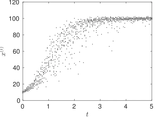
intrinsic variability in the growth rate and measurement noise. In Figure 1, we show an example data set with x0 = 10, K = 100, I = 10 and a noise level of σ2 = 1 whereφ(i) was drawn from a
normal distribution with mean 2 and variance 0.2.
0 1 2 3 4 5
t
0 20 40 60 80 100 120
x
(
i
)
Figure 1: Example logistic data set with x0 = 10, K = 100, I = 10 and σ2 = 1. Each data point
yj(i) represents a sample from an unidentified individual at a given time.
3.1 Improperly treating the data as individual data
We begin by exploring potential pitfalls when disregarding the fact that the data is indeed aggregate data, which again we emphasize is the common assumption made nearly universally in the literature. Consider a standard experimental set up where the datay={yj}nj=1t is collected by only collecting
a single sample from a new subject at each sampling time. That is, the data is generated exactly as described in the section above withI = 1. Since in this section we are disregarding the fact that the measurements are collected from different individuals and instead assuming that the observations are collected from a single individual over time, we arrive at the standard statistical model given by
yj =x(tj;θ) +j.
In the above equation,x(t) denotes the solution to the (deterministic) logistic equation
dx dt =rx
1− x
K
, x(0) =x0, (3.3)
andj is the measurement error. Clearly there is a difference between how the simulated experiment
the modeling assumptions of how the data is collected and how the data is actually collected experimentally. Thus, one possible approach, which we do not explore in this work, is to attempt to account for this model discrepancy in order to arrive at calibrated parameters who’s associated uncertainty agrees with the distributions of the individual parameters pΦ.
Bayesian estimation is a powerful tool for uncertainty analysis, and here we will illustrate that even a Bayesian procedure leads to false conclusions if one assumes that the data is collected from a single individual when in reality the data is unidentified individual data. Through the means of a Bayesian estimation, we will estimate the unknown parameters θ= (r, x0, K)T in the logistic
model (3.3).
The prior density is denoted by π0(θ), which we take as an uniformed prior, and we further
assume that the measurement errors are independent and identically distributed with a normal distribution having mean 0 and variance σ2. With this assumption the likelihood function is given by
π(y|θ) = 1 (2πσ2
)nt/2
exp
− 1
2σ2
nt
X
j=1
(yj −x(tj;θ))2
, (3.4)
where x(tj;θ) is the solution to the logistic equation. Then the posterior density can be obtained
through
π(θ|y) = π(y|θ)π0(θ)
π(y) =
π(y|θ)π0(θ)
R
Rpπ(y|θ)π0(θ)dθ
. (3.5)
The posterior density was approximated using the delayed rejection adaptive Metropolis (DRAM) algorithm [23]. In Figure 2, we present the model fit to a data set which was generated with the measurement error variance σ2 = 1. The mean parameters were found to be
r = 1.9562, x0 = 11.0010, K= 97.8998,
0 1 2 3 4 5 t
0 20 40 60 80 100 120
x
(
i
)
Data Model
0.5 1 1.5 2 2.5 3 3.5
r 0
0.5 1 1.5 2 2.5 3
True pdf rposterior
Figure 2: The model fit to a data set with single data point at each sampling time (left) and the posterior density of the growth rate r compared to the true density (right). The grey shaded region around the model fit is the 95% prediction interval resulting from the Bayesian estimation procedure.
3.2 Parametric estimation - model with the correct distribution
We re-emphasize that our goal is to estimate the unknown values ofx0, K,µΦ, andσΦgiven the data
sety(ji). In this first example, we take the simplest approach by correctly assuming the distribution of the individual growth ratesφ(i). That is, we generate our data by sampling the growth rate from a normal distribution with meanµΦ = 2 and varianceσΦ2 = 0.2, and we assume in our mathematical
model that the growth rate is normally distributed. The inverse problem was solved according to equations (2.11) and (2.12) where Ψ = (µ, σ). The moments of the model x(t;x0, K, µ, σ) were
obtained through a SC method. In applications, there may be either experimental evidence or biologically relevant assumptions that may guide the choice of a distribution for the individual parametersφ(i). We will discuss the case of a nonparametric estimation of the unknown densitypΦ
in a later section.
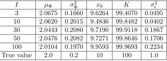
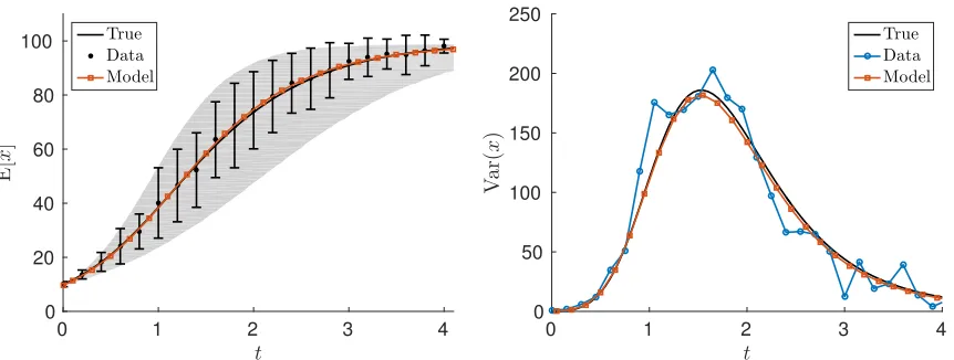
A modest measurement noise ofσ2 = 1 is initially considered. We see from Table 1 that we are able to recover all of the parameters quite well, even with a relatively small number of individual data points at each time point. In general, the estimates improve as the number of individuals sampled at each time increases. In Figure 3, we compare the expected value of the data over time with the resulting model fit (the expected value of the RDE (3.2)), and for comparison we show the true expected value of the RDE withµΦ = 2 andσΦ2 = 0.2. The same comparison for the variance
is also shown in Figure 3.
I µΦ σΦ2 x0 K σ2
3 2.0675 0.1660 9.6264 99.4070 0.0495 10 2.0620 0.2015 9.4836 99.8482 0.0402 30 2.0443 0.2080 9.7190 99.9118 0.1867 50 2.0476 0.2082 9.7271 99.8646 0.1706 100 2.0104 0.1970 9.9593 99.9693 0.2234
True value 2.0 0.2 10 100 1.0
Table 1: Estimated values for the logistic model example with measurement noise level σ2
= 1.
0 1 2 3 4
t
0 20 40 60 80 100
E
[
x
]
True Data Model
0 1 2 3 4
t
0 50 100 150 200 250
V
a
r(
x
)
True Data Model
Figure 3: The fit of the expected value of the RDE model to the mean data and the true expected value of the RDE (left), and the fit of the variance of the RDE model to the variance of the data and the true variance of the RDE withI = 100 and a measurement noise level ofσ2 = 1.
I µΦ σ2Φ x0 K σ2
3 2.0897 0.1762 9.4342 99.3468 1.3008 10 2.0582 0.2089 9.5680 99.9755 1.4208 30 2.0417 0.2127 9.7705 99.9530 2.1629 50 2.0450 0.2130 9.7529 99.9105 2.1755 100 2.0085 0.2004 9.9939 100.0305 2.3386
True value 2.0 0.2 10 100 4.0
Table 2: Estimated values for the logistic model example with measurement noise level σ2 = 4. Both the simulated data and the model are assumed to have a normally distributed growth rate.
I µΦ σ2Φ x0 K σ2
3 2.1649 0.1980 8.7711 99.0550 15.4414 10 2.0518 0.2144 9.7421 100.2071 22.0233 30 2.0378 0.2156 9.8703 99.9581 22.6175 50 2.0376 0.2157 9.8034 99.9554 23.0953 100 2.0047 0.2024 10.0612 100.1363 22.7998
True value 2.0 0.2 10 100 25.0
Table 3: Estimated values for the logistic model example with measurement noise level σ2 = 25. Both the simulated data and the model are assumed to have a normally distributed growth rate.
Even in the presence of an increase in the measurement noise, our estimation procedure performs remarkable well for this example. In Tables 2 and 3 we present the results obtained with σ2 = 4 and 25, respectively.
3.3 Parametric estimation - model with a misspecified distribution
discrepancy in our formulation. We first consider the case where the log-normal distribution has the parameters (µΦ, σ2Φ) = (0.5,0.075) so that the mean and variance of the true distribution are
1.7117 and 0.2282, respectively. Next we take (µΦ, σ2Φ) = (0.3,0.1) as the parameters of the
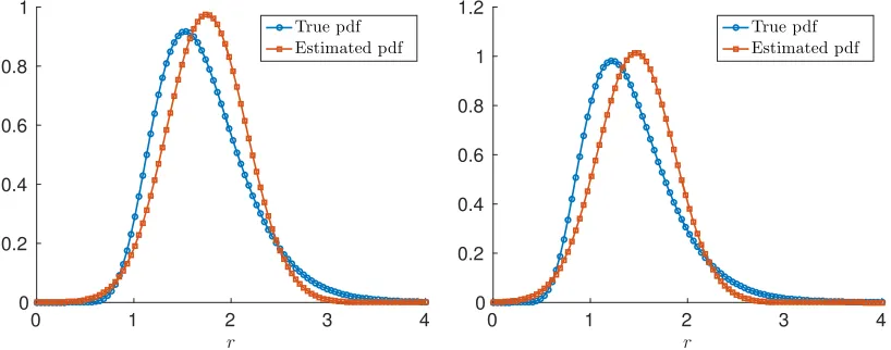
log-normal distribution so that the mean and variance are 1.4191 and 0.2118, respectively. The results of the estimated mean and variance of the distribution are presented in Table 4. We see that we obtain close approximations for the mean value and the carrying capacity; however, the variance is under approximated in both cases, more so for the second case. This is due to the fact that the log-normal distribution becomes more one sided with the choice of (µΦ, σΦ2) = (0.3,0.1). We
expect that if we attempt to use a symmetric (in this case a normal) distribution to approximate the moments of a non-symmetric distribution (here a log-normal distribution), then our approximations will diverge from the true moments. The disparity between the approximated and true moments depends upon the degree to which the true distribution is asymmetric.
I E[pΦ] Var[pΦ] K 100 1.7363 0.1839 99.9172 True value 1.7117 0.2282 100
100 1.4177 0.1530 99.3526 True value 1.4191 0.2118 100
Table 4: Estimated values for the logistic model example. The data is simulated using a log-normally distributed growth rate with measurement noise σ2 = 1, while the model is assumed to have a normally distributed growth rate.
0 1 2 3 4
r 0
0.2 0.4 0.6 0.8 1
True pdf Estimated pdf
0 1 2 3 4
r 0
0.2 0.4 0.6 0.8 1 1.2
True pdf Estimated pdf
Figure 4: The estimated normal probability density to the true log-normal probability density with parameters (µΦ, σΦ2) = (0.5,0.075) (left) and (µΦ, σΦ2) = (0.3,0.1) (right) with I = 100 in both
cases.
3.4 Nonparametric estimation
Using the logistic growth example, Liouville’s equation gives
∂u ∂t +
∂ ∂x
φx1− x
K
u= 0
u(0, x, φ) =u0(x, φ),
(3.6)
∂u ∂t +φx
1− x
K
∂u
∂x =φ
2x K −1
u
u(0, x, φ) =u0(x, φ).
(3.7)
As we mentioned previously, this is a first order linear equation, and we can solve it explicitly using the method of characteristics. The characteristic curves are described by the system of ordinary differential equations
dt
dξ = 0, t(ξ= 0, ν, ρ) = 0, dx
dξ =φx(1−x/K), x(ξ = 0, ν, ρ) =ν, dφ
dξ = 0, φ(ξ = 0, ν, ρ) =ρ, du
dξ =φ(2x/K−1)u, u(ξ = 0, ν, ρ) =u0(ν, ρ).
Solving this system gives
u(ξ, ν, ρ) =u0(ν, ρ)
νeρξ−ν+K K
2
e−ρξ, (3.8)
where
ξ =t, ρ=φ, ν(t, x, φ) = Kx
eφt(K−x) +x. (3.9)
Then, we obtain the probability density for x(t) by
pX(t, x) =
Z
Ω
u(t, ν(t, x, φ), φ)dφ
=
Z
Ω
u0(ν(t, x, φ), φ)
ν(t, x, φ)eφt−ν(t, x, φ) +K K
2
e−φtdφ.
(3.10)
If we assume thatX0 and Φ are independent and have probability densitiespX0 andpΦ, respectively, then their joint pdf is given by u0(x, φ) =pX0(x)pΦ(φ).
For simplicity, we assume that pX
0 is known. What follows can readily be extended to the situation where both pΦ and pX0 are unknown. However, we remark that in the case wherepX0 is unknown, if one has ample data collected at time t= 0, then the density ofpX
0 can be estimated directly from the data by either a parametric or nonparametric approach so long as X0 and Φ are
independent.
By (2.13) we have that
pΦ≈p
M
Φ =
M
X
m=1
wm`m(φ),
thus, we obtain
u0(x, φ)≈uM0 (x, φ) =pX0(x)p
M
Φ (φ) =pX0(x)
M
X
m=1
Substituting this expression into (3.10) gives
pX(t, x)≈p
M
X(t, x) =
Z
Ω
pX0(ν)
M
X
m=1
wm`m(φ)
νeφt−ν+K K
2
e−φtdφ. (3.12)
Given data points pjk for the density of x(t) at timetj, the inverse problem is then given by
(θ,bwb) = argmin
(θ,w)∈Θ
J(θ, w), (3.13)
where the cost functional is now defined as
J(θ, w) =
nx
X
k=1
nt
X
j=1
pjk(yj(i))−pMX(tj, xk)
2
. (3.14)
To simulate the data, the procedure is the same as described in Section 3. In this case however, the number of sampling times is set tont= 51, the initial condition was taken asX0∼ N(µX0, σ
2
X0), withµX0 = 20, σ
2
X0 = 1, and the measurement error variance and the carrying capacity are set to
σ = 1 and K= 100, respectively.
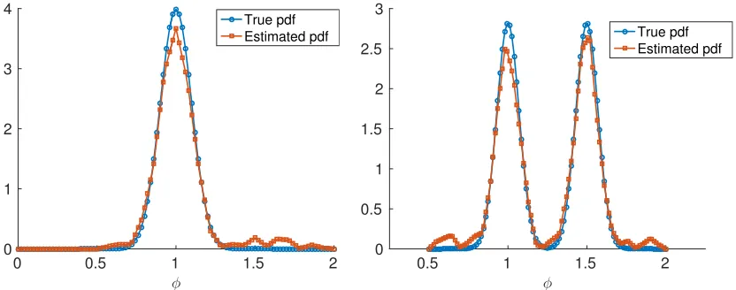
We first consider the case where the true probability density of Φ was taken to be normally distributed with mean and variance µΦ = 1 and σ2Φ = 0.01, respectively. In the left panel of
Figure 5, we show an example of the evolution of the probability density of x(t) over time. The number of approximating spline functions was set to M = 20, and with this we obtained a good estimation for the true density (see Figure 6), and the estimated value for the carrying capacity wasK = 99.9733.
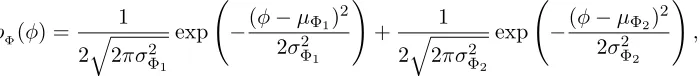
Next we consider the case where the probability density of Φ was that of a Bi-Gaussian distri-bution, which is given by
pΦ(φ) = 1 2q2πσΦ2
1
exp −(φ−µΦ1)
2
2σΦ2
1
!
+ 1
2q2πσΦ2
2
exp −(φ−µΦ2)
2
2σΦ2
2
!
,
with µΦ1 = 1.0, µΦ2 = 1.5, and σ
2 Φ1 = σ
2
Figure 5: The probability densitypX(t, x) obtained from the data pointsyj(i)with noise levelσ = 1
wherepΦ is taken to be normal (left) and Bi-Gaussian(right).
0 0.5 1 1.5 2
φ 0
1 2 3 4
True pdf Estimated pdf
0.5 1 1.5 2
φ 0
0.5 1 1.5 2 2.5 3
True pdf Estimated pdf
4
Applications to a PBPK model
In this section we apply our methods to an experimental data set in which the concentration of 1,1’-Dioctadecyl-3,3,3’,3’-Tetramethylindotricarbocyannine Iodide dye-encapsulated nanoparticles (DIR-NPs) was collected in mice. The concentrations were measured in the liver, spleen, kidney, and plasma. The data was taken from [14] in which a PBPK model was developed specially for this experiment; the in vivo experiment is described fully in [14, 16]. In the experiment, at each observation time point the organs were harvested from three mice. Thus, we have three replicate measurements for the concentration of each measured compartment at each observation time point which provide an estimate of the mean and variance of the concentration over time.
We begin by modifying the original deterministic model proposed in [14] to better account for the accumulation of the drug concentration in the plasma compartment. DIR-NPs were injected into each mouse at the tail at a concentration of 5 mcg/mL and the plasma concentration measurement was collected by submandibular bleeding. In [14], the model developed by Gilkey et al. treats the injection as a step input att= 0. The authors acknowledge that this leads to a discrepancy between the model and the experimental data which exhibits a lag time in the uptake into the plasma, but justify their treatment by observing that the data and model agree after several hours have passed. We propose the following adjustment to the model to better account for the lag time in the uptake of the drug. We define a new state D(t) to account for the amount of the available mass of the DIR-NPs which is taken up by the plasma. We assume that the initial concentration in the plasma is 0, and that the drug enters the plasma through a linear source term. The model accounts for the concentration of NPs in the plasma, liver, kidney, spleen and an “other” compartment. The other compartment represents the remainder of the connective pathways in the body. It is assumed that the absorption by the various tissues is thermodynamically limited rather than rate limited, resulting in first order absorption terms. The modified model is given as
dCP(i) dt =
1
VP
hC(i)
L
R(Li)
Q(Li)+ C
(i)
S
R(Si) QS+
CK(i) R(Ki)
QK+
CO(i) RO
QO
−CP(i)(Q(Li)+QS+QK+QO) +c(i)D(i)
i
dCL(i) dt =
1
VL
h
CP(i)(Q(Li)−QS) +
CS(i) R(Si)
QS+
CO(i) RLO
QO
−C
(i)
L
R(Li)
(Q(Li)+QO)
i
dCS(i) dt =
1
VS
h
CP(i)QS+
CO(i) R(SOi)
QO
−C
(i)
S
R(Si)
(QS−QO)
i
dCK(i) dt =
1
VK
h
CP(i)QK+
CO(i) RKO
QO
− C
(i)
K
R(Ki)
(QK+QO+KK(i))
i
dCO(i) dt = 1 VO h QO
CP(i)−C
(i)
O
RO
i
dD(i) dt =−c
(i)D(i).
(4.1)
with CP(i)(0) = CL(i)(0) = CS(i)(0) = CK(i)(0) = CO(i)(0) = 0, D(i)(0) = D0, where Cz(i) denotes the
concentration of nanoparticles in the organ z and for individuali, Qz is the volumetric flow rate
of plasma through organ z, Vz is the volume of organ z, and KK its the clearance rate from the
to be population level parameters. A log-normal distribution was chosen for each individual level parameter since each parameter must be non-negative in order to be biologically feasible.
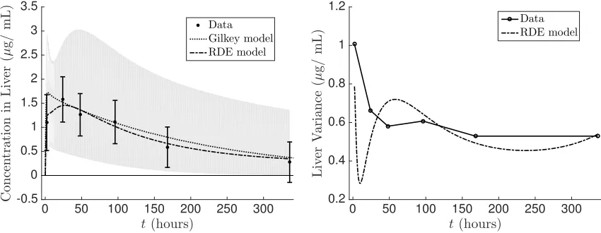
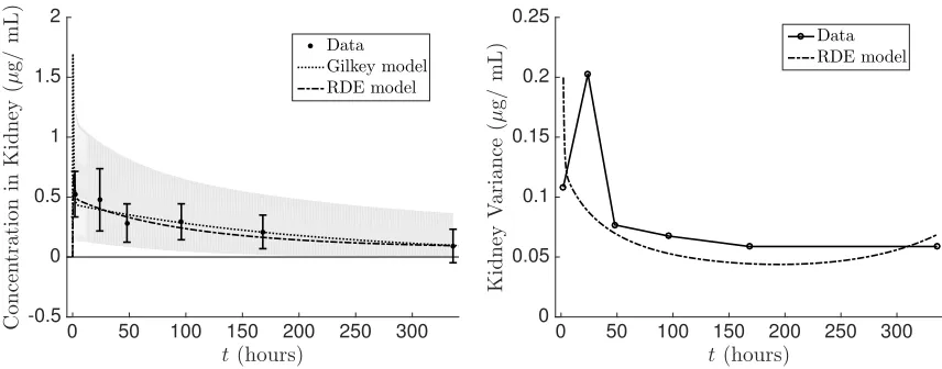
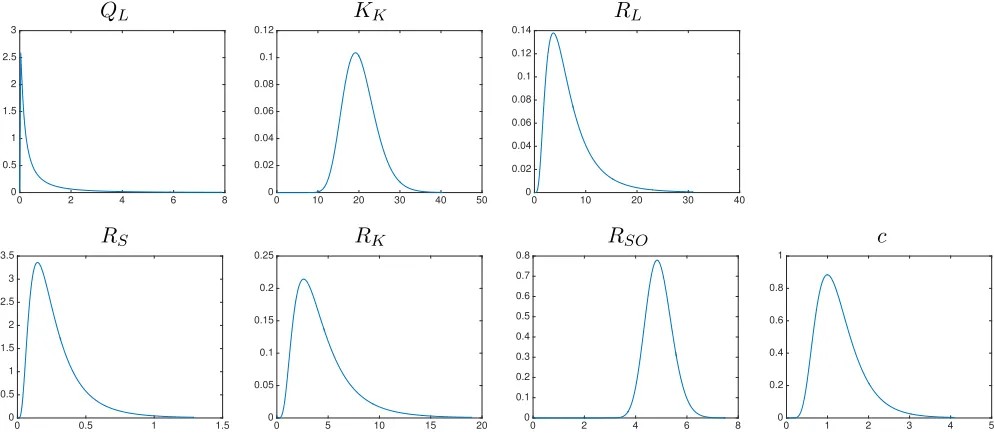
The time varying mean and variance of the resulting RDE system (4.1) were estimated using stochastic collocation in which a sparse grid Gauss-Hermite quadrature rule was used. The mean concentration as well as the standard deviation were fit to the experimental values according to the cost function (2.12). In Figures 7–10 we show the fit of the mean and the variance of the RDE system (4.1) to the experimental data. Additionally, we compare the fit of the original deterministic model (referred to as the Gilkey model in the legend) to the mean of the experimental data. The estimated individual parameter distributions are given in Figure 11. We observe that the RDE model captures the mean data similar to the Gilkey model fort >5. The modified dosing term not only provides a better fit to the initial data points (t <5) but also allowed for the initial non-zero variance values in Figures 7–10. Directly estimating the distribution of the individual parameters in the RDE model allow us to obtain excellent approximations of the variance in the liver and kidney, a reasonable approximation to the spleen, and a fair fit to the plasma prior tot = 5. We are not able to replicate the experimental variance in the plasma after 5 hours. This may be in part due to the fact that the model itself (either the Gilkey model or our modification used here) does not conserve the mass of the administered dose of NPs. If the mass were conserved, we may be able to better account for the variability in the plasma concentration, but adjusting the model to that degree is beyond the scope of this paper and is left for future work.
0 5 10 15 t(hours) -1 0 1 2 3 4 5 C o n ce n tr a ti o n in P la sm a ( µ g / m L ) Data Gilkey model RDE model
0 5 10 15
t(hours) 0 0.1 0.2 0.3 0.4 0.5 0.6 0.7 P la sm a V a ri a n ce ( µ g / m L ) Data RDE model
Figure 7: The observed concentration of nanoparticles in the plasma compared to the model fits using the original deterministic model and the expected value of the RDE system (4.1) (left). The variance computed from three replicate measurements and the fit to the computed variance of the RDE system (4.1) (right).
0 50 100 150 200 250 300
t(hours) -0.5 0 0.5 1 1.5 2 2.5 3 3.5 C o n ce n tr a ti o n in L iv er ( µ g / m L ) Data Gilkey model RDE model
0 50 100 150 200 250 300
t(hours) 0.2 0.4 0.6 0.8 1 1.2 L iv er V a ri a n ce ( µ g / m L
) DataRDE model
0 50 100 150 200 250 300 t(hours) 0 0.2 0.4 0.6 0.8 1 C o n ce n tr a ti o n in S p le en ( µ g / m L ) Data Gilkey model RDE model
0 50 100 150 200 250 300
t (hours) 0.01 0.02 0.03 0.04 0.05 0.06 0.07 0.08 0.09 S p le en V a ri a n ce ( µ g / m L
) DataRDE model
Figure 9: The observed concentration of nanoparticles in the spleen compared to the model fits using the original deterministic model and the expected value of the RDE system (4.1) (left). The variance computed from three replicate measurements and the fit to the computed variance of the RDE system (4.1) (right).
0 50 100 150 200 250 300
t(hours) -0.5 0 0.5 1 1.5 2 C o n ce n tr a ti o n in K id n ey ( µ g / m L ) Data Gilkey model RDE model
0 50 100 150 200 250 300
t(hours) 0 0.05 0.1 0.15 0.2 0.25 K id n ey V a ri a n ce ( µ g / m L ) Data RDE model
QL KK RL
0 2 4 6 8
0 0.5 1 1.5 2 2.5 3
0 10 20 30 40 50
0 0.02 0.04 0.06 0.08 0.1 0.12
0 10 20 30 40
0 0.02 0.04 0.06 0.08 0.1 0.12 0.14
RS RK RSO c
0 0.5 1 1.5
0 0.5 1 1.5 2 2.5 3 3.5
0 5 10 15 20
0 0.05 0.1 0.15 0.2 0.25
0 2 4 6 8
0 0.1 0.2 0.3 0.4 0.5 0.6 0.7 0.8
0 1 2 3 4 5
0 0.2 0.4 0.6 0.8 1
Figure 11: The estimated log-normal distributions for the individual parameters.
5
Concluding remarks
In summary, we have developed a methodology that accounts for parameter variation due to inter-individual variability for the case of repeated measurements of unidentified subjects. Obtaining repeated measurements from unidentified subjects is a common practice in many physiological ex-periments, and the methodology developed in this work agrees conceptually with the experimental design. Using a logistic example with synthetic data we have illustrated how this methodology can be implemented using both a parametric and nonparametric representation for the unknown indi-vidual parameter distributions. Additionally, we used experimental data obtained from repeated measurements of the concentrations of an administered dose of nano particles in a mouse to further illustrate the feasibility of the application of our methods to a recently developed PBPK model. We observed that accounting for the inter-individual variability as outlined in this work leads to differences (typically larger ranges) in the predicted quantities of interest compared to traditional methods which ignore the contribution of inter-individual variability. Recognizing and capturing this uncertainty may prove to be invaluable in the risk assessment of future experiments.
6
Acknowledgements
This work has been supported in part by the US Department of Education Graduate Assistance in Areas of National Need (GAANN) under grant number P200A120047 and in part by the Air Force Office of Scientific Research under grant numbers AFOSR 12-1-0188 and AFOSR FA9550-15-1-0298, and in part by the National Science Foundation under Research Training Grant (RTG) DMS- 1246991 and in part under NSF Undergraduate Biomathematics grant number DBI-1129214.
References
Biology, 64:97–131, 2002.
[2] H.T. Banks. Functional Analysis Framework for Modeling, Estimation and Control in Science and Engineering. Chapman and Hall/CRC Press, Boca Raton, FL, 2012.
[3] H.T. Banks and K.L. Bihari. Modeling and estimating uncertainty in parameter estimation.
Inverse Problems, 17:95–111, 2001.
[4] H.T. Banks, B.G. Fitzpatrick, L.K. Potter, and Y. Zhang. Estimation of probability distri-butions for individual parameters using aggregate population data. In Stochastic Analysis, Control, Optimization and Applications: a Volume in Honor of W.H. Fleming. Birkhauser, Boston, 1999.
[5] H.T. Banks, S. Hu, and W.C. Thompson. Modeling and Inverse Problems in the Presence of Uncertainty. Taylor/Francis-Chapman/Hall-CRC Press, Boca Raton, FL, 2014.
[6] H.T. Banks and F. Kappel. Spline approximations for functional differential equations. J. Differential Equations, 34:496–522, 1979.
[7] H.T. Banks, Z.R. Kenz, and W.C. Thompson. A review of selected techniques in inverse problem nonparametric probability distribution estimation. J. Inverse and Ill-Posed Problems, 20:429–460, 2012.
[8] H.T. Banks and L.K. Potter. Probabilistic methods for addressing uncertainty and variability in biological models: Application to a toxicokinetic model.Mathematical Biosciences, 192:193– 225, 2004.
[9] H.A. Barton, W.A. Chiu, R.W. Setzer, M.E. Anderson, A.J. Bailer, F.Y Bois, R.S. DeWoskin, S. Hays, G. Johanson, N. Jones, G. Loizou, R.C. MacPhail, C.J. Portier, M. Spendiff, and Y.M. Tan. Characterizing uncertainty and variability in physiologically based pharmacokinetic models: state of the science and needs for research and implementation.Toxicological Sciences, 99:395–402, 2007.
[10] J.C. Caldwell, M.V. Evans, and K. Krishnan. Cutting edge pbpk models and analyses: pro-viding the basis for future modeling efforts and bridges to emerging toxicology paradigms.
Journal of Toxicology, 2012, 2012.
[11] M. Davidian and A.R. Gallant. The nonlinear mixed effects model with a smooth random effects density. Biometrika, 80(3):475–488, 1993.
[12] S. Donnet and A. Samson. A review on estimation of stochastic differential equations for pharmacokinetic/pharmacodynamic models. Advanced Drug Delivery Reviews, 65(7):929–939, 2013.
[13] T. Eissing, J. Lippert, and S. Willmann. Pharmacogenomics of codeine, morphine, and morphine-6-glucuronide. Molecular Diagnosis & Therapy, 16(1):43–53, 2012.
[14] M.J. Gilkey, V. Krishnan, L. Scheetz, X. Jia, A.K. Rajasekaran, and P.S. Dhurjati. Physiolog-ically based pharmacokinetic modeling of fluorescently labeled block copolymer nanoparticles for controlled drug delivery in leukemia therapy. CPT: Pharmacometrics & Systems Pharma-cology, 4(3):167–174, 2015.
[16] V. Krishnan, X. Xu, S.P. Barwe, X. Yang, K. Czymmek, S.A. Waldman, R.W. Mason, X. Jia, and A.K. Rajasekaran. Dexamethasone-loaded block copolymer nanoparticles induce leukemia cell death and enhance therapeutic efficacy: a novel application in pediatric nanomedicine.
Molecular Pharmaceutics, 10(6):2199–2210, 2012.
[17] M.J. Lindstrom and D.M. Bates. Nonlinear mixed effects models for repeated measures data.
Biometrics, pages 673–687, 1990.
[18] J. Lippert, M. Brosch, O. Kampen, M. Meyer, H.U. Siegmund, C. Schafmayer, T. Becker, B. Laffert, L. G¨orlitz, S. Schreiber, P.J. Neuvonen, M. Niemi, J. Hampe, and L. Kuepfer. A mechanistic, model-based approach to safety assessment in clinical development. CPT: Pharmacometrics & Systems Pharmacology, 1(11):1–8, 2012.
[19] G. Loizou, M. Spendiff, H.A. Barton, J. Bessems, F.Y. Bois, M.B. dYvoire, H. Buist, H.J. Clewell, B. Meek, U. Gundert-Remy, G. Goerlitz, and W. Schmitt. Development of good modelling practice for physiologically based pharmacokinetic models for use in risk assessment: the first steps. Regulatory Toxicology and Pharmacology, 50(3):400–411, 2008.
[20] J. Pinheiro and D. Bates. Mixed-effects Models in S and S-PLUS. Springer Science & Business Media, New York, NY, 2006.
[21] M.H. Schultz. Spline Analysis. Prentice-Hall, Englewood Cliffs, NJ, 1973.
[22] L.B. Sheiner. The population approach to pharmacokinetic data analysis: rationale and stan-dard data analysis methods. Drug Metabolism Reviews, 15(1-2):153–171, 1984.
[23] R.C. Smith. Uncertainty Quantification: Theory, Implementation and Application. SIAM, Philadelphia, PA, 2013.
[24] T.T. Soong. Random Differential Equations in Science and Engineering. Academic Press, New York, NY, 1973.