©
DOI: 10.1534/genetics.104.034181
Mapping Multiple Quantitative Trait Loci by Bayesian Classification
Min Zhang,* Kristi L. Montooth,
†,1Martin T. Wells,*
,‡Andrew G. Clark
†and Dabao Zhang
§,2*Department of Biological Statistics and Computational Biology, Cornell University, Ithaca, New York 14853,†Department of Molecular Biology and Genetics, Cornell University, Ithaca, New York 14853,‡Department of Statistical Science, Cornell University,
Ithaca, New York 14853 and§Department of Biostatistics and Computational Biology, University of Rochester Medical Center, Rochester, New York 14642
Manuscript received July 30, 2004 Accepted for publication November 1, 2004
ABSTRACT
We developed a classification approach to multiple quantitative trait loci (QTL) mapping built upon a Bayesian framework that incorporates the important prior information that most genotypic markers are not cotransmitted with a QTL or their QTL effects are negligible. The genetic effect of each marker is modeled using a three-component mixture prior with a class for markers having negligible effects and separate classes for markers having positive or negative effects on the trait. The posterior probability of a marker’s classification provides a natural statistic for evaluating credibility of identified QTL. This approach performs well, especially with a large number of markers but a relatively small sample size. A heat map to visualize the results is proposed so as to allow investigators to be more or less conservative when identifying QTL. We validated the method using a well-characterized data set for barley heading values from the North American Barley Genome Mapping Project. Application of the method to a new data set revealed sex-specific QTL underlying differences in glucose-6-phosphate dehydrogenase enzyme activity between two Drosophila species. A simulation study demonstrated the power of this approach across levels of trait heritability and when marker data were sparse.
T
HE fact that we can map variation in complex phe- tion (DoebleyandStec1991). As such, QTL mapping is not simply a gene-finding tool. QTL mapping provides notypes to chromosomal regions by exploiting thelinkage between random genetic markers and causal critical information regarding quantitative evolutionary genetic processes.
genetic variants in related individuals has long been
understood. Since the formalization of statistical ap- Traditional approaches to QTL mapping primarily involve multiple regression models and maximum-likeli-proaches to this type of inference by Lander and
Botstein (1989) and the advent of high-throughput hood estimation and are powerful for detecting QTL
of moderate to large effect. However, detecting multiple methodologies for constructing genetic maps with high
marker density, quantitative trait locus (QTL) mapping smaller genetic effects that may modify or interact with larger effects is necessary and remains a challenge. in organisms from crops to mice has provided a rich
These smaller effects are important, as they can poten-knowledge of genes underlying important
socioeco-tially enhance crop breeding and further our under-nomic traits. It also has provided a better understanding
standing of genetic background effects on complex dis-of the genetic architecture dis-of complex traits both within
ease. Quantifying the abundance of these types of effects and between species. QTL mapping promises the
im-for any given trait also fills a gap in our knowledge provement of crops of international importance, such
regarding the distribution of genetic effects. as drought-resistant rice (for review see Price and
The most popular approach for QTL mapping is
in-Courtois1999;Priceet al.2002), and the advancement
terval mapping (IM). Proposed by Lander and
Bot-of treatments for complex physiological diseases like
stein(1989), IM conducts likelihood-ratio tests for each
high blood pressure (Sugiyamaet al.2001). QTL
map-possible QTL by densely gridding chromosomes using ping has also been used to map traits that may be the
linkage information in the available marker data. It tac-target of intense selection both in natural populations,
itly assumes that the trait of interest is regulated by a such as sexually dimorphic pigmentation patterns in
single gene. Under this single-QTL model, IM may fail Drosophila (Koppet al.2003), and in crop
domestica-to separate closely linked QTL and instead report ghost QTL that have no true effect on the trait (Knottand
Haley 1992; Martinez and Curnow 1992; Wright
1Present address:Department of Ecology and Evolutionary Biology,
Brown University, Providence, RI 02912. and Kong 1997). Furthermore, epistatic interactions
2Corresponding author: Department of Biostatistics and
Computa-between QTL are not identified by IM. Many
ap-tional Biology, University of Rochester Medical Center, 601 Elmwood
proaches have therefore been developed on the basis
Ave., Box 630, Rochester, NY 14642.
E-mail: [email protected] of multiple-QTL models that generalize the single-QTL
model. Conditioning on selected markers outside a re- that have detectable positive effects on the phenotypic values), a negative-effect class (including all QTL that gion of interest to account for background effects,
com-posite-interval mapping (CIM) and multiple-QTL map- have detectable negative effects on the phenotypic val-ues), and a negligible-effect class (including all non-ping (MQM) search for QTL across a series of intervals
covering chromosomes (Jansen1993;Zeng1993, 1994; QTL markers and all nondetectable QTL). In modeling the population distribution for each class, we construct
Jansen and Stam 1994). Multiple-interval mapping
(MIM) directly regresses the trait on a set of markers, a three-component mixture prior distribution for the effect of each investigated marker. The proposed proce-which densely grid the chromosomes (Kaoet al.1999).
Identification of multiple QTL is subject to the statistical dure is able to incorporate thea prioriinformation that most of the markers under investigation have negligible issue of variable selection (Piepho and Gauch 2001;
Broman and Speed 2002; Sillanpa¨a¨ and Corander effect on the trait and that the positive-effect class and
negative-effect class may have different sizes. Two trun-2002), and Bayesian methodology using Markov chain
Monte Carlo algorithms has been developed for this cated Gaussian distributions are used to model the population distributions for the positive-effect class and problem (Satagopanet al.1996;Sillanpa¨a¨andArjas
1998; Stephensand Fisch1998; Ball2001; Senand negative-effect class. Using an a priori inverse gamma distribution for their variance parameters, the
corre-Churchill2001;Xu2003;Yiet al.2003).
The Bayesian approach provides a natural framework sponding prior distributions are essentially truncated
t-type distributions so as to be sufficiently flexible heavy-for modeling multiple QTL, as it can accommodate
multiple imputation of missing values in phenotypes as tailed prior distributions. This incorporates the empiri-cal observation that the distribution of genetic effects well as genotypes and include all markers as random
variables in a single model. The ability to incorporate is heavy tailed (LopezandLopez-Fanjul1993; Keight-ley 1994;Keightley andOhnishi1998). These par-available information into QTL mapping and update
with newly observed data is an advantage provided tially informative prior distributions not only shrink the estimates of the QTL effects toward zero to avoid the uniquely by Bayesian analysis. Access to powerful
com-putational resources and efficient algorithms makes it “curse of dimensionality,” but also allow for the estima-tion of thea posterioriprobabilities that a marker belongs realistic to implement Bayesian analysis, and the direct
interpretation of the results from a Bayesian analysis to the positive-effect class, the negative-effect class, or the negligible-effect class. Although point estimates of also makes it particularly applicable for the scientific
community (Shoemaker et al. 1999; Beaumont and these a posteriori probabilities provide information to discover the corresponding effects’ classes (as inYiet al.
Rannala2004).
Many Bayesian QTL-mapping methods capitalize on 2003), the distributional departure from probability 0.5 delivers additional information to help investigators the complex reversible-jump Markov chain Monte Carlo
algorithm (Green1995) to estimate the number of QTL make informed decisions when determining QTL sig-nificance. As a graphical display, we propose a “heat and their effects on the trait (Satagopan et al.1996;
Sillanpa¨a¨andArjas1998;StephensandFisch1998). map” to visually display the posterior probabilities of
membership in the positive-, negative-, or negligible-To avoid the problematic issue of Markov chain mixing
introduced by uncertain dimensionality of parameter effect class.
To validate our proposed approach we analyzed pub-space,Yiet al.(2003) developed an alternative Bayesian
method for identifying multiple QTL in experimental licly available data from a study of agronomic traits in a doubled-haploid (DH) population of barley (North designs based on stochastic search variable selection
(George and McCulloch 1993). For those markers American Barley Genome Project). Data sets simulated
across three trait heritabilities suggest that the proposed that have negligible effects on the trait, they assume
the effects follow mean-zero Gaussian distributions with approach is powerful for detecting a broad range of QTL effects, even when genotype data are missing. As arbitrarily specified small standard deviations. In this
way the dimension of the parameter space is fixed and a further application, we used the method to detect sex-specific QTL underlying glucose-6-phosphate dehydro-a more trdehydro-actdehydro-able Gibbs sdehydro-ampler cdehydro-an be constructed. The
posterior probability that a marker has a large effect is genase activity in a set of recombinant inbred introgres-sion lines betweenDrosophila simulansandD. sechellia. estimated and used to indicate significance of QTL.
However, by using Gaussian distributions with small standard deviations to model negligible effects,Yiet al.
THE MODEL AND BAYESIAN CLASSIFICATION (2003) reduce the efficiency in the mapping procedure,
resulting in small posterior probabilities for the effects Multiple-linear-regression model: We focus on map-ping multiple QTL in a set of homozygous lines, such of QTL on the trait even if the corresponding effects
are large. as doubled-haploid lines or recombinant inbred lines, generated from an initial cross between two isogenic We propose a new Bayesian framework to identify
zygous individuals, such as backcrosses or intercrosses. tion for modeling and incorporating prior information as shown below.
Assume genotypic data formmarkers and phenotypic
data for one complex trait of interest are collected from Assume the population distribution for the positive-effect class and the negative-positive-effect class to beF⫹and
nindividuals. Further assume themmarkers are densely
located on the chromosomes of interest such that puta- F⫺, respectively. Let p⫹ be the probability for any
marker to be included inᏼ() andp⫺be the
probabil-tive QTL will be cotransmitted with some of thesem
mark-ers. Subject to additive main effects from putative QTL, ity for any marker to be included inᏺ(). Then, each
jwith j僆 ᏼ() [orj 僆 ᏺ()] can be considered as the phenotypic value of individuali(yi) is modeled as
independently sampled from an unknown distribution
yi⫽ ⫹
兺
mj⫽1
jxj i⫹εi, (1) F⫹(orF⫺). Hence, we have a three-component mix-ture prior distribution for the effect of each marker; that is,
where is the overall mean,xj iis the genotypic value of thejth marker of individuali, andεiis the disturbance
error from environmental factors, which is assumed to jⵑ iid
(1⫺ p⫹⫺p⫺)␦{0}⫹p⫹F⫹⫹p⫺F⫺, (2) be distributed asN(0, 2
ε). Therefore,jdescribes the
where␦{0}is a Dirac function with value one at zero and main effect of thejth putative QTL.
value zero otherwise. This three-component mixture When the markers are widely spaced across the
ge-prior distribution is able to incorporate thea priori infor-nome, we can tightly grid the genome by imputing
geno-mation that most of the markers under investigation types between markers (Lander and Botstein 1989;
have negligible effects on the trait and that the sizes of
Ball2001; Sen and Churchill 2001;Kilpikari and
the positive-effect class and negative-effect class may be
Sillanpa¨a¨2003;Xu2003). This is equivalent to
assum-different. Note that this prior does not use indicators ing that the genotypic values of some markers are
miss-to specify each marker’s classification and avoids the ing for all individuals. In practice, some marker
geno-unnecessary sampling of the indicator variables in the types are also partially missing. All of these missing
Gibbs sampler. genotypic values can be inferred using the known
link-In practice, we can simply take F⫹⫽N⫹(0,2⫹),
age information and the available marker genotype data
F⫺⫽ N⫺(0, 2⫺). The probability density functions of
(seeJiangandZeng1997). This model can incorporate
the two truncated Gaussian distributionsN⫹(,2) and
both observed and imputed marker information.
N⫺(,2) are, respectively,
Identifying QTL from the markers under
investiga-tion using the above multiple-linear-regression model is ⌽(/)⫺1
√
22 exp冦
⫺(x⫺ )2
22
冧
I[x⬎ 0], equivalent to selecting variablesxj i, which have nonzerocoefficientsj. Although previous approaches for QTL
mapping have considered classical model selection ap- ⌽(⫺/)⫺1
√
22 exp冦
⫺(x⫺ )2
22
冧
I[x⬍0]. (3) proaches in statistics (e.g.,Kao et al. 1999; Zenget al.1999;Ball2001;BromanandSpeed2002), effects of
The generality of the above priors can be guaranteed imputed missing values on model selection have been
by putting a further hierarchy of prior distributions on largely ignored due to the potential difficulty. Classical
the hyperparameters2
⫹and2⫺; that is, assuming the
model selection approaches are severely challenged
prior distributions when there are numerous highly correlated markers
⫺2
⫹ⵑ⌫(⫹,φ⫹), ⫺⫺2 ⵑ⌫(⫺,φ⫺). (4)
and a small sample size. We therefore propose a Bayes-ian classification method that incorporates the
impor-These priors (e.g., setting⫹⫽ ⫺⫽ 0.5 andφ⫹⫽ tant prior information that the QTL effects of most φ
⫺ ⫽ 2 for 21-distributions) lead to truncated t-type genotypic markers are negligible and naturally exploits
distributions that are heavy tailed for the positivejand the linkage information in the genetic linkage map to
negativej, respectively. They will shrink the estimated impute missing values.
effects toward zero but at the same time provide the
Bayesian framework:We first classify all markers
un-flexibility to model the population distributions for der investigation into three classes, the positive-effect ᏼ
() andᏺ(). Furthermore,t-type prior distributions classᏼ()⫽{j:j⬎0}, the negative-effect classᏺ()⫽
confer desirable decision-theoretic properties for the {j :j ⬍ 0}, and the negligible-effect class ᐆ() ⫽ {j :
Bayes estimators (Fourdrinieret al.1998).
j ⫽ 0}. Therefore, for each j in ᏺ() or ᏼ(), the
Results from previous QTL mapping may provide in-corresponding marker has a negative or positive effect
formation about the probability of a marker having a on the trait, respectively, and for each j in ᐆ() the
positive, negative, or negligible effect on the trait. This corresponding marker has no detectable effect on the
a prioriinformation may be incorporated into the follow-trait. Often, many markers may belong to the
negligible-ing conjugate prior distribution forp⫹andp⫺,
effect classᐆ(), and the sizes of the positive-effect class
and the negative-effect class may be small and varied. (p⫹,p⫺, 1⫺ p⫹⫺p⫺)ⵑDirichlet(,φ,).
founda-In the case that no prior information is available forp⫹ p˜j⫹⫽P(j⬎0|yn,xn,,⫺j,p⫹,p⫺,2ε,2⫹,2⫺), andp⫺, we can assume each is uniformly distributed
p˜j⫺⫽P(j⬍0|yn,xn,,⫺j,p⫹,p⫺,2ε,2⫹,2⫺). on the interval [0, 1] [i.e., the joint Dirichlet(1, 1, 1)
distribution, which describes the characteristics of no The chain {p˜(t)
j⫹,t⫽1, 2, . . . ,T} or {˜p(jt⫺),t⫽ 1, 2, . . . , prior information]. Typically the number of markersm T} can be used to evaluate whether thejth marker has
is large relative to the sample sizen, and it is unrealistic a positive or negative effect on the trait, respectively. to assume bothp⫹andp⫺are uniformly distributed Furthermore, the posterior probabilities pj⫹ ⫽ P(j ⬎ on the interval [0, 1]. Instead, we can restrict bothp⫹ 0|yn, xn) and pj⫺ ⫽ P(j ⬍ 0|yn,xn) can be estimated andp⫺to be smaller than min(冑n/m, 1). This restric- from these two chains, and it is these posterior probabili-tion also accounts for the sample size. Accordingly, the ties that provide information on the classification of prior distribution forp⫹andp⫺should follow a trun- markers into the positive- and negative-effect classes. In cated Dirichlet distribution. The intercepthas a uni- other words, these posterior probabilities can be used form prior while2
ε has a prior proportional to 1/2ε, as statistics for evaluation of whether or not a marker
both of which are noninformative. These priors, to- is linked to a QTL for the trait of interest. A value of gether with priors defined by (2)–(5), provide a proper the posterior probabilitypj⫹⬎0.5 indicates that thejth joint posterior distribution for the model (1), which is marker has a positive effect on the trait, while a value shown in theappendix. ofpj⫺⬎0.5 indicates a negative effect of thejth marker
Single-site Gibbs sampler:A single-site Gibbs sampler on the trait. Otherwise, we infer that thejth marker has can be developed following the above formulation of a nondetectable effect on the trait.
the Bayesian model. Letyncollect all phenotypic values A heat map (Figure 1) can be used to graphically of the trait andxncollect all genotypic values of the m view the values ofpj⫹andpj⫺at different percentiles of
putative QTL. Let⫽(1, . . . ,m),⫺jbeexcluding their posterior distributions, allowing the investigator to
j, and x⫺j,i ⫽ (x1i, . . . , xj⫺1,i, xj⫹1,i, . . . , xmi). Each visualize the posterior probabilities of a marker having a iteration of the Gibbs sampler proceeds by recursively positive or negative effect with different levels of strin-drawing each missing genotypic value and each parame- gency. In this way, the heat map provides a visual device ter value from its full conditional posterior distribution. for determining the significance of QTL. The values of Details for the implementation of the Gibbs sampler pj⫹andpj⫺at different percentiles of their distributions with the imputation of missing genotypic values are are shown using a color scheme that maps a value of presented in theappendix. zero to white, 0.5 to orange, and 1 to red. A spot at the This Gibbs sampler starts from initial values for miss- ␣ ⫻100 percentile in the top (or bottom) half of the ing genotypic values and all other parameters. Initial heat map with color ranging from orange to red implies values for missing genotypes can be sampled on the that the probability of the corresponding marker be-basis of the nearest neighboring observed genotypic longing to the positive-effect (or negative-effect) class values and available genetic linkage information. Initial is⬎0.5 with a credibility of (1⫺ ␣)⫻100%. For exam-values for and2
ε can simply take the sample mean ple, the first marker in Figure 1 can be inferred as a and variance ofyn. Regressing the phenotypic value of QTL with negative effect at the 90% credibility level but the trait only on thejth genotypic value provides suit- not at the 99% credibility level, as its tenth percentile able initial values for thej. Then, the initial values for spot in the bottom half is red (pj⫺⬎ 0.5), but its
first-2
⫹and 2⫺can be calculated by using min(2
冑
n,m) percentile spot in the bottom half is less than that of components of the initial values of , which have the yellow (pj⫺⬍0.5). The heat map provides flexibility to largest absolute values. investigators, allowing them to be more or lessconserva-Starting from these initial values and running the tive when identifying QTL.
Gibbs sampler for a sufficient burn-in period (5000 steps For eachj, we may use the chain {(t)
j ,t⫽1, 2, . . . , in our analysis), the Gibbs sampler reaches stationarity T} to estimate its value. However, we are more interested that can be confirmed by diagnostic tools (Cowlesand in estimating the size ofjgiven the class it belongs to.
Carlin1996). Each subsequent iteration of the Gibbs The corresponding chain may provide an unreliable
sampler provides a random draw of the missing values estimate because of the limited number of(t)
j in some and all other parameters from their posterior distribu- of the three classes. We propose to calculate the median tions. All the draws after the burn-in period form a values at each iteration of the Gibbs sampler,
multivariate Markov chain on which inferences can be
˜j⫹⫽median([j|j⬎0,yn,xn,,⫺j,p⫹,p⫺,ε2,2⫹,2⫺]); based.
Marker classification and effect estimation:After the ˜
j⫺⫽median([j|j⬍0,yn,xn,,⫺j,p⫹,p⫺,2ε,2⫹,2
⫺]).
sufficient burn-in period, we run the above Gibbs
sam-pler for Tadditional iterations. Then, for eachj, we Then, if j 僆 ᏼ() [or j 僆 ᏺ()], the chain {˜(jt⫹), have two assumably stationary chains, i.e., {p˜(t)
j⫹,t⫽ 1, t⫽1, 2, . . . ,T} [or {˜(jt⫺),t⫽ 1, 2, . . . ,T}] will provide an estimate ofj. With˜j⫹,˜j⫺,˜j⫹, and˜j⫺defined 2, . . . ,T} and {p˜(t)
Figure 1.—Heat map for posterior probabilities pj⫹⫽ P(j⬎ 0|yn, xn) and
pj⫺⫽P(j⬍0|yn,xn). These are the proba-bilities of being in either the positive or the negative genetic-effect class. The val-ues ofpj⫹andpj⫺at different percentiles of the posterior distribution are shown using different colors according to the color scheme on the right. If the color of
pj⫹ (or pj⫺) at the ␣ ⫻ 100 percentile ranges from orange to red, it implies that the probability of thejth marker belong-ing to the positive-effect (or negative-effect) class is ⬎0.5 with a credibility of (1⫺ ␣)⫻100%.
in theappendix, the two median values can be calcu- cofactors is not our primary interest. We can simply partition all nonmarker factors into different groups lated as
such that the coefficients for all factors within the same
˜j⫹⫽ ˜j⫹ ⫺ ⌽⫺1(0.5⌽(˜
j⫹/˜j⫹))˜j⫹,
group can be assigned independently and identically distributed prior distributions. The Bayesian framework
˜j⫹⫽ ˜j⫺ ⫹ ⌽⫺1(0.5⌽(⫺˜
j⫺/˜j⫺))˜j⫺,
and Gibbs sampler can therefore be developed adap-where⌽(·) is the cumulative distribution function of a
tively. standard normal distribution, and⌽⫺1(·) is its inverse
Instead of collecting one observation, we may collect function.
replicate observations for each inbred line. For this type
Extensions: Our Bayesian framework can be easily
of clustered data, efficiency consideration and non-adapted to include imputation of genotypes between
marker cofactors may prevent summarizing the observa-markers, as well as epistatic interactions. The extensions
tions from each line into one phenotypic value. The of the genetic model to non-Gaussian phenotypic data
above genetic model and Bayesian framework are quite may complicate the development of the corresponding
amenable to this type of data. Since individuals from Gibbs sampler. However, this type of data could be
han-the same line share marker genotypes, a common value dled conceptually. In particular, drawing random
sam-should be imputed to each missing marker genotype ples ofjfrom its full conditional distribution may lose
for all individuals within the same line. its easy computability. In this case, while p˜j⫹ and p˜j⫺
may be calculated numerically, computation of˜j⫹and
˜j⫺ may need to be approximated using a
Metropolis-VALIDATION AND SIMULATION type algorithm.
Days to heading QTL in barley:To validate the model, The model (1) and its Bayesian framework can be
we analyzed line means for days from planting until further extended. Continuous and discrete nonmarker
emergence of 50% of heads on main tillers for 145 cofactors, can be incorporated into the
multiple-linear-barley doubled-haploid lines that were genotyped for regression model. For example, letziinclude, for
indi-127 markers across seven linkage groups (Tinker et
viduali, all nonmarker cofactors that affect the
corre-al.1996). Yi et al. (2003) analyzed this data set using sponding phenotypic value. Then, subject to additive
stochastic search variable selection. Using a critical main effects from putative QTL and nonmarker factors,
threshold value of 0.5 for the posterior probability of a the phenotypic value of individuali(yi) can be modeled
marker being in the nonnegligible class,Yiet al.(2003) as
mapped QTL at markers I.12, III.5, IV.9, V.10, and VI.5
yi⫽ ⫹
兺
mj⫽1
jxj i⫹zTi␥⫹ εi, (the Roman number refers to the linkage group and the Arabic number refers to the marker index within the group). However, simply using the point estimates where␥describes the effects of the nonmarker factors.
of these posterior probabilities to indicate significance Usually, we incorporate nonmarker factors into the
of the corresponding markers ignores the variability of above model to control for their potential effects on
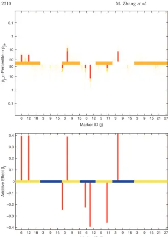
Figure2.—Results of Bayesian classifica-tion for heading trait in the North Ameri-can Barley Genome Mapping Project. Shown are the heat map for posterior prob-abilitiespj⫹andpj⫺(top) and the estimated additive effects (bottom). In the top and bottom, the central lines represent differ-ent chromosomes by using colors alternat-ing between orange and white and between yellow and blue, respectively. The marker identifications (IDs) along thex-axis are the IDs within the corresponding chromo-somes.
these posterior probabilities from probability 0.5 pro- score obtained from 1000 permutations of the pheno-typic data. In concordance with results obtained from vides a more informative approach for QTL detection.
With our three-component prior approach, QTL are our method and byYiet al.(2003), IM identified signifi-cant QTL around markers I.12, III.5, IV.9, and V.10 mapped by using the distributional departure of the
posterior probabilitiespj⫹andpj⫺from probability 0.5. plus several additional QTL around markers IV.5, VI.3, and VII.18. Background markers for CIM were chosen Figure 2 shows the result of mapping QTL by our
pro-posed approach. Markers III.5 and IV.9 are significant by forward selection with background elimination re-gression using inclusion and exclusion probabilities of with credibility level at 90%, but the evidence for
sig-nificance of markers I.12, VI.5, and V.10 is weak. In 0.1. CIM identifies QTL around markers I.6, I.12, III.5, III.9, III.12, IV.9, V.10, and VII.18 and better localizes this example, if we simply threshold the medians of
posteriorspj⫹andpj⫺at 0.5, 8 markers, including those the QTL to a more narrow region around marker IV.9. Implementation of MIM using the forward/backward above, appear to have significant nonnegligible effects,
demonstrating the drawback to using a point estimate selection method with a significance level of 0.01 identi-fied 15 QTL. Using the standard Bayes information cri-as a critical threshold for QTL detection.
We further analyzed the data set using IM, CIM, and terion model selection, we were able to detect three additional QTL.
MIM implemented in QTL Cartographer 2.0 (Wanget
QTL, with the results from CIM and MIM depending upon the model selection criterion employed. In partic-ular, MIM detects many more significant QTL than the other methods. A comprehensive simulation study is necessary to fully assess the relative strengths and weak-nesses of these different approaches. However, one ad-vantage of the method we propose is better evaluation of the significance of a QTL.
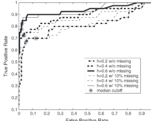
Simulation study:The ability to detect QTL is strongly influenced by the trait heritability, with most statistical methods being able to detect QTL for highly heritable traits. However, for many phenotypes of interest, the genetic component of the variance may be small relative to the environmental variance, making QTL detection challenging. In these cases, even QTL of relatively large effect may be difficult to detect when the random envi-ronmental effects on the trait are also large. To assess
Figure3.—ROC curves plotting the true-vs. the false-posi-the performance of our approach we analyzed 10
ran-tive rates from the simulation study. The asterisks correspond domly generated QTL models with phenotypes
simu-to mapping QTL by reading the median values from the distri-lated under three levels of heritability and with either butions ofp
j⫹andpj⫺. The flat part of the ROC curve corre-no or 10% missing data. The data sets simulated were sponds to mapping QTL using more liberal decision rules to allow a higher false-positive rate to improve the true-positive for 225 recombinant inbred lines with three linkage
rate. On the other hand, more conservative QTL mapping groups containing a total of 27 markers. The number of
may prefer some decision rules at the steep part of the ROC recombination events per chromosome per generation
curve, where the false-positive rate is decreased at a cost to was drawn from a Poisson distribution with mean equal the detection of true positives.
to the length of the chromosome in morgans (Haldane
1919).
The 10 QTL models each contained four QTL with set group. The receiver operating characteristic (ROC) curves (Metz 1978) are drawn by using the Bayesian effects drawn from a ⌫(2, 1) distribution. At the jth
QTL of the ith line, the effect is defined as 2␣j for classification approach on each 10-data set group (Fig-ure 3). ROC curves assess the trade-off between the true-marker genotypeAA (i.e.,␣i j⫽ ␣j) and 0 for marker
genotypeaa(i.e.,␣i j⫽0). The genotypic value of a line and false-positive rates. Our ability to detect the 40 QTL effects drawn from a⌫(2, 1) distribution improved sig-is the sum of these effects across the four true QTL,
and the genetic variance (2
g) is the sample variance of nificantly with increasing heritability and was only slightly affected by missing values. Using the median the genotypic values across the lines. The phenotypic
value for each line (Yi) is calculated asYi⫽2兺4j⫽1␣i j⫹ values from the distributions ofpj⫹ andpj⫺ as critical threshold values for mapping QTL is equivalent to
mak-εi, where the random environmental effect (εi) is drawn fromN(0,2
ε). The environmental variance (2ε) is de- ing decisions at the turning part of the ROC curve (i.e.,
Figure 3, asterisks). More liberal QTL mapping may fined as ((1⫺h2)/h2)2
g, where h2 is the heritability
(0⬍ h2 ⬍1). We simulated phenotypic values for the favor some decision rules at the flat part of the ROC curve to improve the true-positive rate by allowing an 10 QTL models using h2 ⫽ 0.2, 0.4, and 0.6, which
correspond to the environmental variance being 4 increased false-positive rate. This liberal approach to QTL mapping may be particularly useful when the goal times, 1.5 times, and two-thirds of the genetic variance.
Simulations were performed using QTL Cartographer is to identify large numbers of QTL candidates, such as in marker-assisted selection programs (Spelman and version 1.13 (Bastenet al.1994, 1999), and simulated
data sets with and without missing data were analyzed Bovenhuis1998;Beuzenet al.2000;Dekkersand
Hos-pital2002). However, as is often the case, more
conser-by our Bayesian classification method to infer the
true-and false-positive rates. vative QTL mapping will require decision rules at the steep part of the ROC curve, decreasing the false-posi-In total there were 10 mapping data sets with 40 true
QTL simulated across the range of heritabilities, both tive rate but potentially missing some true QTL. The heat map for posterior probabilitiespj⫹ andpj⫺ is de-with and de-without missing data. With sufficient
recombi-nation between markers, each QTL should be detected signed to allow investigators to make these types of deci-sions when scanning genomes for QTL.
only by its neighboring markers. We therefore
consid-ered any significant markers not directly neighboring Given a trait’s heritability, QTL detection will also depend upon the magnitude of the single-QTL effect. simulated QTL as false positives. This will inflate our
classification approach. The true-positive rates here are calculated by counting only those QTL with effects higher than each given effect size. With heritability 0.2, conservative QTL mapping makes it difficult to identify QTL even if these QTL have large effects. Mapping QTL by reading the median values from the distributions of
pj⫹ and pj⫺ identified large-effect QTL, but this ap-proach may lead to more false positives (Figure 3). With increasing heritability, more conservative decision rules could be adopted to lower false-positive rates without loss of power to detect large-effect QTL (Figure 4). Note that many markers that are one marker away from the markers neighboring QTL were significant and classi-fied as false positives according to our stringent defini-tion of true positives. A looser definidefini-tion of true positives will significantly improve the results reported in Figures 3 and 4.
DATA ANALYSIS
Glucose-6-phosphate dehydrogenase (EC1.1.1.49, G6PD) catalyzes the conversion of glucose-6-phosphate (G6P) to 6-phospho-d-glucono-1,5-lactone, shunting G6P from the main backbone of glycolysis through the pentose-phosphate pathway and creating reducing power for the cell in the form of NADPH. In Drosophila, patterns of nucleotide variation at G6PD (Eanes et al. 1993, 1996), as well as covariance in enzyme activities of G6PD and its neighboring enzyme, 6-phosphogluconate dehy-drogenase, across Drosophila species (ClarkandWang
1994), suggest that G6PD activity may come under selec-tion in natural populaselec-tions. Enzyme activities may evolve via mutations at the enzyme-encoding loci or rather through mutations at trans-acting loci that alter the quantity or function of the enzyme. QTL mapping pro-vides a way to determine whether variation in enzyme activity (Mitchell-Olds and Pedersen 1998;
Mon-toothet al.2003) or protein quantity (Damervalet al.
1994) is the result of genetic variationcisortransto the enzyme-encoding locus.
Introgression lines between closely related species allow us to map QTL underlying interspecific differ-ences in quantitative traits. We quantified male and female G6PD activity in 221 inbred introgression lines between the sibling speciesD. simulans andD. sechellia
that were genotyped at 28 markers across the X, second, and third chromosomes. Details for the construction and genotyping of these lines can be found in
Dermit-zakiset al.(2000) andCivettaet al.(2002). We
mea-sured G6PD activity as in vitro maximal activity from Figure4.—True-positive ratevs. effect size (␣) at different whole-fly homogenates using a standard spectrophoto-heritabilities:h2⫽0.2 (top),h2⫽0.4 (middle), andh2⫽0.6
metric assay to monitor the NADPH that accumulates (bottom). The true-positive rates are calculated by counting
when G6P is converted to 6-phospho-d -glucono-1,5-lac-only those QTL with effects higher than the given effect size
tone (Clark andKeith1989). The data set for male (x-axis). The different lines refer to the different decision
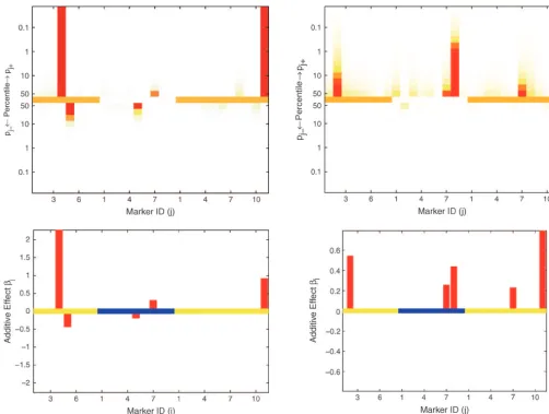
Figure5.—Results of Bayesian classification for male G6PD (left) and female G6PD (right) enzyme activities. Shown are the heat map for posterior probabilitiespj⫹andpj⫺(top) and the estimated additive effects (bottom). In the top and bottom, the central lines represent different chromosomes by using colors alternating between orange and white and between yellow and blue, respectively. The marker IDs along thex-axis are the IDs within corresponding chromosomes.
We applied our Bayesian classification approach to 5). The residual variances for G6PDM and G6PDF were estimated to be 0.5697 and 0.7089, respectively. Because detect interspecific QTL for G6PD activity and to
deter-mine whether the same loci underlie G6PD activity in the phenotypic values are standardized in our analysis, the markers and covariates in this model explainedⵑ43 males and females. This is a particularly challenging
data set for QTL detection, as the percentage of missing and 29% of the phenotypic variation in G6PD activity for males and females, respectively.
genotype data is high (18%) and, due to the nature of
the introgression (see Dermitzakis et al. 2000), the To assess the performance of our method with this data set, we simulated five data sets using the observed frequency of theD. sechelliagenotype at certain markers
can range from 2 to 66%. There were also a number marker genotypes and the parameter estimates from the above analysis for both G6PDM and G6PDF. Analyz-of covariates that we needed to incorporate into the
model to control for both biological (fly weight and ing data simulated in this fashion can reveal the effects of imputing missing genotype data, as the missing data total protein content) and experimental effects.
We identified a QTL on the tip of the right arm of are imputed independently for each simulated dataset. Among the two most outstanding effects on G6PDM in chromosome 3 (marker III.11) that has strong effects
on G6PD activity in both males and females (Figure 5). Figure 5, marker I.4 was strongly significant in four of five simulated data sets and was mildly significant in the It is interesting to observe that while this QTL had the
same magnitude of effect in both sexes, there was an fifth data set, while marker III.11 was highly significant in all simulated data sets. The remaining three weak additional X-linked QTL (marker I.4), distinct from the
effect than marker III.11, more missing genotype data where the normalizedlp-norm is bounded by(
John-stone andSilverman 2004). We conjecture that the
for marker I.4 than for marker III.11 slightly
compro-mised its significance in mapping QTL. estimation methods proposed here achieve an optimal estimation rule as the sample size increases and as The estimated effects on G6PDF were much smaller
(Figure 5). The most outstanding effect on G6PDF at goes to zero, in which sense it adapts automatically to the parameter space’s sparseness.Johnstoneand
Sil-marker III.11 was strongly significant in three out of
five simulated data sets and mildly significant in the verman(2004) study a general class of estimation prob-lems in sparse parameter spaces and show that a two-other two data sets. Because of unbalanced genotypes
at marker I.2 (ⵑ1:50), marker I.2 is seldom significant component mixture prior is adaptive and has some optimal estimation properties. The modeling strategy in the five simulated data sets, although it is only slightly
smaller in effect size than marker III.11. Nonnegligible using a two-component mixture prior has been quite successful in attacking similar issues of false positives effects in the initial data analysis were detected as weakly
significant effects in one of the five simulated G6PDM and false negatives in gene expression identification
(Zhanget al.2004) where one needs to identify a small
data sets and in two of the five G6PDF data sets.
As illustrated in this simulation study, equal segrega- number of differentially expressed genes from a large number of candidates.
tion of marker genotypes can improve the ability to
accurately map QTL. The extent of missing genotype The specification of the prior distribution for the genetic effects is critical and can influence the perfor-data may also affect QTL detection, particularly when
the marker genotypes are unbalanced. False nonnegligi- mance of the Bayesian approach to QTL mapping. Moti-vated by the above observations and the need to incorpo-ble effects seldom appear in the results from our
ap-proach and, when observed, their significance as QTL rate biologically relevant information into the prior specification of the genetic effects, we developed a was marginal.
three-component mixture prior on the basis of a natural classification of the marker effects (i.e., positive-, nega-DISCUSSION
tive-, and negligible-effect classes) in a new Bayesian inference framework. The posterior probability of a
The three-component mixture prior as a natural
speci-fication of genetic effects: Model selection based on marker belonging to one of the three categories is a natural statistic for assessing the significance of any multiple-regression models of phenotypic data on
multi-ple genetic markers is increasingly accepted as a general marker being linked to a QTL for the trait of interest. This posterior probability of a marker’s classification framework for mapping multiple QTL, with a large
number of proposed methodologies being developed can be sharply inferred, and the marker effect on the phenotype can also be efficiently estimated using the (e.g., see Hoeschele 2001; Piepho and Gauch2001;
Broman and Speed 2002; Sillanpa¨a¨ and Corander proposed Gibbs sampler. Furthermore, the uncertainty
associated with these estimates is naturally available 2002;Yi2004). QTL mapping is an inherently
challeng-ing problem. Large amounts of misschalleng-ing marker data, from the corresponding posterior distributions, provid-ing an advantage over classical approaches. Simulation due to failure in genotyping or selective genotyping,
are quite common in practice. When markers are sparse, experiments revealed that the approach is powerful for QTL detection and has relatively low false-positive rates, the missing genotype information between markers
must also be inferred (Kaoet al.1999;Zenget al.1999). even when there are large amounts of missing data. The three-component prior approach that we advo-In addition, the number of markers to test can be very
large relative to the number of observed individuals cate for here has four significant advantages over exist-ing methods for QTL inference. First, three-component
(Meuwissenet al.2001;Xu2003), a problem that has
been notoriously difficult in statistics. priors incorporate the known information that most markers are not cotransmitted with QTL or their QTL The majority of genetic markers across a genome will
not be linked to QTL for the trait of interest. From a effects are not detectable, which is important in control-ling false-positive inference. In particular, if the number statistical theory perspective, the parameter space in a
QTL identification problem is quite sparse. Most classi- of available markers is on the same scale as the number of lines (or even if there are more markers than lines), cal methods for QTL mapping work well for a small
number of QTL candidates. The challenge is then to it is necessary to incorporate this prior expectation of rarity of QTL to guarantee the model identifiability in develop an easy-to-implement framework for QTL
map-ping that efficiently detects sparse effects with a suffi- multiple-linear regression. Second, the three-compo-nent prior approach is flexible and allows an imbalance ciently low false-positive rate, precisely estimates their
effects, and does so in the face of missing data and small between sizes/distribution of positive- and negative-effect classes. Third, unlike the two-component priors numbers of observations. Two typical parameter spaces
used to model sparseness are “nearly black” spaces, used byYiet al.(2003), we classify all effects into three classes and describe the population distribution of each where the proportion of the nonzero parameter
variable selection, which has difficulty in specifying 2003). A recent analysis of differential allelic expression inD. melanogasterandD. simulanshybrids found thatcis -many prior parameters and relies on assorting of each
acting effects could largely explain interspecific expres-marker into either the small-effect or the large-effect
sion differences between the two closely related Dro-class. Note thatXu (2003) models each putative QTL
sophila species (Wittkoppet al.2004). The interspecific effect with a Gaussian distribution having its own
vari-G6PD QTL identified in our analysis havetrans-acting ance parameter and further specifies noninformative
effects in both males and females, suggesting that differ-priors for each variance parameter to avoid the above
ences in G6PD activity have evolved betweenD. simulans
difficulty. However, the efficiency in extracting
informa-andD. sechellia via genetic variants located away from tion from the data may be lowered by ignoring that
the enzyme-encoding locus. QTL mapping is an impor-most markers have negligible effects on the trait. Tuning
tant tool in our continued attempts to understand the parameters is a general problem with reversible-jump
role ofcis- andtrans-acting genetic effects in the evolu-Markov chain Monte Carlo that we can avoid in our
tion of gene expression, protein quantity, and enzymatic method. The fourth advantage of our approach is that
activity regulation. the Gibbs sampler exports parameters ˜j⫹, ˜j⫺, p˜j⫹,
Implementation and extension of the Bayesian
classi-and p˜j⫺, which can be used to make inference more
fication approach:The proposed Gibbs sampling algo-efficiently than the-chain only.
rithm for our Bayesian classification approach is
imple-Identification of sex-specific QTL inD. simulansand
mented in MATLAB as software called QTLBayes (free D. sechellia: Application of our Bayesian classification
for academic usage), which, due to its flexibility, can approach to a data set of metabolic enzyme activities
be readily applied to most QTL data. The framework from inbred introgression lines revealed QTL
underly-is currently for the analysunderly-is of inbred lines derived from ing G6PD activity differences between the closely related
two inbred parental lines, and it can accommodate mul-Drosophila species,D. simulansandD. sechellia. We
iden-tiple covariates, as well as replicate measures for individ-tified a QTL on the tip of the right arm of chromosome
uals from the same line. The heat map provides an 3 at cytological position 99E2 where theD. sechelliaallele
informative visual tool for identifying significant QTL increased G6PD activity in both males and females. We
at varying levels of stringency. also identified a male-specific QTL on the X
chromo-One disadvantage of Bayesian analysis is the intensive some at cytological position 7C1, which is distinct from
computation involved (Nakamichiet al.2001). If there the X-linked G6PD enzyme-encoding locus at
cytologi-are only a small number of missing values, the computa-cal position 18D13. These results suggest that genetic
tion will not be an issue. Although imputation of missing differences in G6PD activity betweenD. simulansandD.
data can be easily handled statistically within our
frame-sechelliaare caused bytrans-acting and sex-specific genetic
work, imputation of large amounts of missing genotype effects.
data may be computationally slow. An alternative strat-In D. melanogaster sex-specific genetic architecture is
egy is to assume that there is at most one QTL between common. Sex-specific QTL underlie neuro-sensory
phe-each pair of neighboring markers and adopt the com-notypes (Long et al. 1995; Mackay and Fry 1996;
posite space representation byYi(2004). Prior
specifi-Fanaraet al.2002), as well as life-history traits, such as
cation can also impact algorithm performance in Bayes-longevity (Nuzhdinet al.1997) and starvation resistance ian analysis. The only informative priors in our analysis
(Harbisonet al.2004). Sex-specific genetic effects also are the specification of inverse gamma distributions for
shape global expression variation withinD. melanogaster 2
⫹and⫺2 to provide heavy-tailed priors for the
distri-(Anholtet al. 2003) and between Drosophila species bution of genetic effects. When available, additional
(Ranzet al.2003). Our results demonstrate that in Dro- information can be readily incorporated into the prior sophila these sex-specific genetic effects also contribute specification, increasing the efficiency of estimation. to interspecific differences between species in metabolic While the software currently analyzes data from iso-processes. genic lines, the model can be readily modified to accom-Genome-wide analyses of gene expression, protein modate a variety of experimental designs. The approach abundance, and function are shedding light on the rela- could also be extended to more complicated cases in tive contribution ofcis- andtrans-acting genetic variants QTL mapping, such as clustered data, multiple pheno-to both inter- and intraspecific variation. QTL mapping types, and pairwise epistasis. Detecting epistatic interac-results indicate thattrans-acting effects predominate in- tions between pairs of QTL is an important challenge, traspecific variation in yeast (Schadtet al. 2003) and driven by the biological interest in detecting genetic mouse (Brem et al. 2002) expression profiles, protein interactions, but hampered by the extreme multiplicity quantity in maize (Damervalet al.1994), and enzyme of tests in performing an exhaustive search. The ability activity in bothD. melanogaster(Montoothet al.2003) of our approach to select variables in the case of many and Arabidopsis (Mitchell-OldsandPedersen1998). tests with a small number of observations makes it possi-However,cis-acting effects are also detected, and in yeast ble to directly extend the approach to identify pairwise
andT. F. C. Mackay, 2002 Vanasco is a candidate quantitative We thank Carlos Bustamante for stimulating the collaboration
be-trait gene for Drosophila olfactory behavior. Genetics162:1321– tween the authors, Hengli Liang for her contribution to the early
1328. stages of this project, and Lei Wang for collection of the primary
Fourdrinier, D., W. E. StrawdermanandM. T. Wells, 1998 On enzyme kinetics data. We also thank Steven D. Tanksley, Gary
the construction of Bayes minimax estimators. Ann. Stat.26: Churchill, Patricia Wittkopp, and two anonymous reviewers for sugges- 660–671.
tions that improved this article. Research support by National Science George, E. I., andR. E. McCulloch, 1993 Variable selection via Foundation (NSF) grant DMS-0204252 to M.T.W. as well as National Gibbs sampling. J. Am. Stat. Assoc.88:881–889.
Institutes of Health grant AI46409 and NSF grant DEB-0242987 to Green, P. J., 1995 Reversible jump Markov Chain Monte Carlo com-putation and Bayesian model determination. Biometrika82:711– A.G.C. is gratefully acknowledged.
732.
Haldane, J. B. S., 1919 The combination of linkage values, and the calculation of distance between the loci of linked factors. J. Genet. 8:299–309.
LITERATURE CITED
Harbison, S. T., A. H. Yamamoto, J. J. Fanara, K. K. Norgaand
T. F. C. Mackay, 2004 Quantitative trait loci affecting starvation
Anholt, R. R. H., C. L. Dilda, S. Chang, J.-J. Fanara, N. H. Kulkarni
et al., 2003 The genetic architecture of odor-guided behavior resistance inDrosophila melanogaster.Genetics166:1807–1823.
Hoeschele, I., 2001 Mapping quantitative trait loci in outbred pedi-inDrosophila: epistasis and the transcriptome. Nat. Genet. 35:
180–184. grees, pp. 599–644 inHandbook of Statistical Genetics, edited by
D. J.Balding, M.Bishopand C.Cannings. John Wiley & Sons,
Ball, R. D., 2001 Bayesian methods for quantitative trait loci
map-ping based on model selection: approximate analysis using the New York.
Jansen, R. C., 1993 Interval mapping of multiple quantitative trait Bayesian information criterion. Genetics159:1351–1364.
Basten, C. J., B. S. WeirandZ-B. Zeng, 1994 Zmap—a QTL cartog- loci. Genetics135:205–211.
Jansen, R. C., andP. Stam, 1994 High resolution of quantitative rapher, pp. 65–66 inProceedings of the 5th World Congress on Genetics
Applied to Livestock Production: Computing Strategies and Software, traits into multiple loci via interval mapping. Genetics136:1447– 1455.
edited by C.Smith, J. S.Gavora, B.Benkel, J.Chesnais, W.
Fairfullet al.Organizing Committee, 5th World Congress on Jiang, C., andZ-B. Zeng, 1997 Mapping quantitative trait loci with dominant and missing markers in various crosses from two inbred Genetics Applied to Livestock Production, Guelph, Ontario,
Canada. lines. Genetica101:47–58.
Johnstone, I. M., andB. W. Silverman, 2004 Needles and straw in
Basten, C. J., B. S. WeirandZ-B. Zeng, 1999 QTL Cartographer.
Department of Statistics, North Carolina State University, Ra- haystacks: empirical Bayes estimates of possibly sparse sequences. Ann. Stat.32:1594–1649.
leigh, NC.
Beaumont, M. A., andB. Rannala, 2004 The Bayesian revolution Kao, C.-H., Z-B. ZengandR. D. Teasdale, 1999 Multiple interval mapping for quantitative trait loci. Genetics152:1203–1216. in genetics. Nat. Rev. Genet.5:251–261.
Beuzen, N. D., M. J. StearandK. C. Chang, 2000 Molecular mark- Keightley, P. D., 1994 The distribution of mutation effects on viability inDrosophila melanogaster.Genetics138:1315–1322. ers and their use in animal breeding. Vet. J.160:42–52.
Brem, R. B., G. Yvert, R. ClintonandL. Kruglyak, 2002 Genetic Keightley, P. D., andO. Ohnishi, 1998 EMS-induced polygenic mutation rates for nine quantitative characters inDrosophila mela-dissection of transcriptional regulation in budding yeast. Science
296:752–755. nogaster.Genetics148:753–766.
Kilpikari, R., andM. J. Sillanpa¨a¨, 2003 Bayesian analysis of
mulitlo-Broman, K. W., andT. P. Speed, 2002 A model selection approach
for the identification of quantitative trait loci in experimental cus associations in quantitative and qualitative traits. Genet. Epi-demiol.25:122–135.
crosses. J. R. Stat. Soc. B64:641–656.
Civetta, A., H. M. Waldrip-DailandA. G. Clark, 2002 An intro- Knott, S. A., andC. S. Haley, 1992 Aspects of maximum likelihood methods for mapping of quantitative trait loci in line crosses. gression approach to mapping differences in mating success and
sperm competitive ability inDrosophila simulansandD. sechellia. Genet. Res.60:139–151.
Kopp, A., R. M. Graze, S. Xu, S. B. CarrollandS. V. Nuzhdin, Genet. Res.79:65–74.
Clark, A. G., andL. E. Keith, 1989 Rapid enzyme kinetic assays of 2003 Quantitative trait loci responsible for variation in sexually dimorphic traits inDrosophila melanogaster.Genetics163:771–787. individualDrosophilaand comparisons of field-caughtD.
melano-gasterandD. simulans.Biochem. Genet.27:263–277. Lander, E. S., andD. Botstein, 1989 Mapping Mendelian factors
underlying quantitative traits using RFLP linkage maps. Genetics
Clark, A. G., andL. Wang, 1994 Comparative evolutionary analysis
of metabolism in nineDrosophila species. Evolution48:1230– 121:185–199 [corrigendum: Genetics136:705 (1994)].
Long, A. D., A. L. Mullaney, L. A. Reid, J. D. Fry, C. H. Langley
1243.
Cowles, M. K., andB. P. Carlin, 1996 Markov chain Monte Carlo et al., 1995 High resolution mapping of genetic factors affecting abdominal bristle number inDrosophila melangogaster.Genetics convergence diagnostics: a comparative review. J. Am. Stat. Assoc.
91:883–904. 139:1273–1291.
Lopez, M. A., andC. Lopez-Fanjul, 1993 Spontaneous mutation
Damerval, C., A. Maurice, J. M. Josse and D. de Vienne,
1994 Quantitative trait loci underlying gene product variation: a for a quantitative trait inDrosophila melanogaster. II. Distribution of mutant effects on the trait and fitness. Genet. Res.61:117–126. novel perspective for analyzing regulation of genome expression.
Genetics137:289–301. Mackay, T. F. C., andJ. D. Fry, 1996 Polygenic mutations in
Drosoph-ila melanogaster: genetic interactions between selection lines and
Dekkers, J. C., andF. Hospital, 2002 The use of molecular genetics
in the improvement of agricultural populations. Nat. Rev. Genet. candidate quantitative trait loci. Genetics144:671–688.
Martinez, O., andR. N. Curnow, 1992 Estimating the locations 3:22–32.
Dermitzakis, E. T., J. P. Masly, H. M. WaldripandA. G. Clark, and the size of the effects of quantitative trait loci using flanking markers. Theor. Appl. Genet.85:480–488.
2000 Non-Mendelian segregation of sex chromosomes in
heter-ospecific Drosophila males. Genetics154:687–694. Metz, C. E., 1978 Basic principles of ROC analysis. Semin. Nucl. Med.8:283–298.
Doebley, J., andA. Stec, 1991 Genetic analysis of the morphological
differences between maize and teosinte. Genetics129:285–295. Meuwissen, T. H., B. J. HayesandM. E. Goddard, 2001 Prediction of total genetic value using genome-wide dense marker maps.
Eanes, W. F., M. KirchnerandJ. Yoon, 1993 Evidence for adaptive
evolution of the G6pd gene in theDrosophila melanogasterand Genetics157:1819–1829.
Mitchell-Olds, T., andD. Pedersen, 1998 The molecular basis of Drosophila simulanslineages. Proc. Natl. Acad. Sci. USA90:7475–
7479. quantitative genetic variation in central and secondary
metabo-lism in Arabidopsis. Genetics149:739–747.
Eanes, W. F., M. Kirchner, J. Yoon, C. H. Biermann, I. N. Wanget
al., 1996 Historical selection, amino acid polymorphism and Montooth, K. L., J. H. MardenandA. G. Clark, 2003 Mapping determinants of variation in energy metabolism, respiration and lineage-specific divergence at the G6pd locus inDrosophila
melano-gasterandD. simulans.Genetics144:1027–1041. flight in Drosophila. Genetics165:623–635.
Nakamichi, R., Y. UkaiandH. Kishino, 2001 Detection of closely
linked multiple quantitative trait loci using a genetic algorithm. Stephens, D. A., andR. D. Fisch, 1998 Bayesian analysis of
quantita-Genetics158:463–475. tive trait locus data using reservible jump Markov chain Monte
Nuzhdin, S. V., E. G. Pasyukova, C. L. Dilda, Z-B. ZengandT. F. C. Carlo. Biometrics54:1334–1347.
Mackay, 1997 Sex-specific quantitative trait loci affecting lon- Sugiyama, F., G. A. Churchill, D. C. Higgins, C. Johns, K. P.
gevity in Drosophila melanogaster.Proc. Natl. Acad. Sci. USA94: Makaritsis et al., 2001 Concordance of murine quantitative
9734–9739. trait loci for salt-induced hypertension with rat and human loci.
Piepho, H.-P., andH. G. Gauch, Jr., 2001 Marker pair selection Genomics71:70–77.
for mapping quantitative trait loci. Genetics157:433–444. Tinker, N. A., D. E. Mather, B. G. Rossnage, K. J. KashaandA.
Price, A. H., andB. Courtois, 1999 Mapping QTLs associated with Kleinhofs, 1996 Regions of the genome that affect agronomic drought resistance in rice: progress, problems and prospects. performance in two-row barley. Crop Sci.36:1053–1062. Plant Growth Reg.29:123–133. Wang, S., C. J. BastenandZ-B. Zeng, 2004 Windows QTL
Cartogra-Price, A. H., J. E. Cairns, P. Horton, H. G. JonesandH. Griffiths, pher 2.0.Department of Statistics, North Carolina State University, 2002 Linking drought-resistance mechanisms to drought avoid- Raleigh, NC (http://statgen.ncsu.edu/qtlcart/WQTLCart.htm). ance in upland rice using a QTL approach: progress and new Wittkopp, P. J., B. K. HaerumandA. G. Clark, 2004 Evolutionary opportunities to integrate stomatal and mesophyll responses. J. changes in cis and trans gene regulation. Nature430:85–88. Exp. Bot.53:989–1004.
Wright, F. A., andA. Kong, 1997 Linkage mapping in experimental
Ranz, J. M., C. I. Castillo-Davis, C. D. MeiklejohnandD. L. Hartl,
crosses: the robustness of single-gene models. Genetics146:417– 2003 Sex-dependent gene expression and evolution of the
Dro-425. sophilatranscriptome. Science300:1742–1745.
Xu, S., 2003 Estimating polygenic effects using markers of the entire
Satagopan, J. M., B. S. Yandell, M. A. NewtonandT. C. Osborn,
genome. Genetics163:789–801. 1996 A Bayesian approach to detect quantitative trait loci using
Yi, N., 2004 A unified Markov chain Monte Carlo framework for Markov chain Monte Carlo. Genetics144:805–816.
mapping multiple quantitative trait loci. Genetics167:967–975.
Schadt, E. E., S. A. Monks, T. A. Drake, A. J. Lusis, N. Cheet al.,
Yi, N., V. GeorgeandD. B. Allison, 2003 Stochastic search variable 2003 Genetics of gene expression surveyed in maize, mouse
selection for identifying multiple quantitative trait loci. Genetics and man. Nature422:297–302.
164:1129–1138.
Sen, S., andG. Churchill, 2001 A statistical framework for
quantita-Zeng, Z-B., 1993 Theoretical basis for separation of multiple linked tive trait mapping. Genetics159:371–387.
gene effects in mapping quantitative trait loci. Proc. Natl. Acad.
Shoemaker, J. S., I. S. PainterandB. S. Weir, 1999 Bayesian
statis-Sci. USA90:10972–10976. tics in genetics: a guide for the uninitiated. Trends Genet.15:
Zeng, Z-B., 1994 Precision mapping of quantitative trait loci. Genet-354–358.
ics136:1457–1468.
Sillanpa¨a¨, M. J., andE. Arjas, 1998 Bayesian mapping of multiple
quantitative trait loci from incomplete inbred line cross data. Zeng, Z-B., C.-H. KaoandC. J. Basten, 1999 Estimating the genetic
Genetics148:1373–1388. architecture of quantitative traits. Genet. Res.74:279–289.
Sillanpa¨a¨, M. J., andJ. Corander, 2002 Model choice in gene Zhang, D., M. T.Wells, C. D.Smartand W. E.Fry, 2004 Bayesian mapping: what and why. Trends Genet.18:301–307. normalization and inference for differential gene expression
Spelman, R. J., andH. Bovenhuis, 1998 Moving from QTL experi- data. J. Comp. Biol.12:391–406. mental results to the utilization of QTL in breeding programmes.
Anim. Genet.29:77–84. Communicating editor: M. W.Feldman
APPENDIX: IMPLEMENTATION OF THE SINGLE-SITE GIBBS SAMPLER
Let the vectoryncollect all phenotypic values of the trait andxncollect all genotypic values of themputative QTL, and let⫽(1, . . . ,m) and⫺jbeexcludingj,x⫺j,i⫽(x1i, . . . ,xj⫺1,i,xj⫹1,i, . . . ,xmi). Denote the conditional distribution ofAgivenBas [A|B] and the marginal distribution ofAas [A]. Each of the conditional distributions below are based on the fact that [A|B]⬀[B|A][A].
Each iteration of the Gibbs sampler can proceed as follows:
0. Specify initial values as described in the Bayesian framework section.
1. Sample each missing genotypic valuexj ifrom its full conditional posterior distribution,
[xj i|yi,x⫺j,i,,,2ε]⬀[yi|x⫺j,i,xj i,,,2ε]⫻[xj i|xj⫺1,i,xj⫹1,i].
2. Samplefrom its full conditional distribution,
|yn,xn,,2 εⵑN
冢
1n
兺
n
i⫽1
冢
yi⫺
兺
mj⫽1
jxj i
冣
,2 ε n
冣
.3. For eachj⫽ 1, . . . ,m, sample jfrom its full conditional distribution,
j|yn,xn,,⫺j,p⫹,p⫺,2ε,2⫹,2⫺ⵑ(1⫺ p˜j⫹⫺p˜j⫺)␦{0}⫹p˜j⫹N⫹(˜j⫹,˜2j⫹)⫹ p˜j⫺N⫺(˜j⫺,˜2j⫺),
where
˜j⫹⫽
2
⫹
兺
ni⫽1xj i(yi⫺ ⫺兺
l⬆jlxl i)2
ε ⫹ ⫹2
兺
in⫽1x2j i,
˜2 j⫹⫽
2
⫹2ε
2
˜j⫺⫽ 2
⫺
兺
ni⫽1xj i(yi⫺ ⫺兺
l⬆jlxl i)2
ε⫹ 2⫺
兺
ni⫽1x2j i,
˜2 j⫺⫽
2
⫺2ε
2
ε⫹ 2⫺
兺
ni⫽1x2j i ,p˜j⫹⫽
2p⫹(˜j⫹/⫹)⌽(˜j⫹/˜j⫹)exp{˜2 j⫹/2˜2j⫹}
1⫺p⫹⫺p⫺⫹2p⫹(˜j⫹/⫹)⌽(˜j⫹/˜j⫹)exp{˜2j⫹/2˜j2⫹}⫹2p ⫺(˜j⫺/⫺)⌽(⫺(˜j⫺/˜j⫺))exp{˜j2⫺/2˜2j⫺} ,
p˜j⫺⫽
2p ⫺(˜j⫺/⫺)⌽(⫺(˜j⫺/˜j⫺))exp{˜2
j⫺/2˜2j⫺}
1⫺p⫹⫺p⫺⫹2p⫹(˜j⫹/⫹)⌽(˜j⫹/˜j⫹)exp{˜2j⫹/2˜j2⫹}⫹2p⫺(˜j⫺/⫺)⌽(⫺(˜j⫺/˜j⫺))exp{˜2j⫺/2˜2j⫺} .
4. Sample 2
εfrom its full conditional distribution,
⫺2
ε |yn,xn,,ⵑ⌫
冢
n2, 2/
兺
ni⫽1
冢
yi ⫺ ⫺
兺
mj⫽1
jxj i
冣
2冣
. 5. Sample p⫹andp⫺from the full conditional distribution,(p⫹,p⫺, 1⫺ p⫹⫺p⫺)|ⵑ Dirichlet(⫹ n˜⫹,φ⫹ n˜⫺,⫹ m⫺ n˜⫹⫺n˜⫺),
wheren˜⫹⫽ #{j:j ⬎0, 1ⱕ jⱕm} andn˜⫺⫽ #{j:j⬍0, 1 ⱕjⱕm}. If the prior distribution ofp⫹and
p⫺is restricted to be less than min(
冑
n/m, 1), the full conditional distribution should be a truncated Dirichletdistribution. 6. Sample 2
⫹and2⫺from the full conditional distributions,
⫺2
⫹|ⵑ⌫
冢
⫹⫹ n˜⫹2 ,
冢
1/φ⫹⫹ 1 2兺
m
j⫽1
2
jI[j⬎0]
冣
⫺1
冣
,⫺2
⫺|ⵑ⌫
冢
⫺⫹n˜ ⫺2 ,
冢
1/φ ⫺⫹ 1 2兺
m
j⫽1
2
jI[j⬍0]
冣
⫺1