Image Denoising Techniques Using Wavelets
S.Y.Pattar
,Associate Professor, Department of Medical Electronics, BMS College of Engineering Bangalore, Karnataka, India
Abstract-The focus of this work is to develop performance-enhancing algorithm for denoising the signal by using wavelet transformation. The earlier methods used for denoising were based on FFT, where signal is transformed in to frequency domain and soft and hard threshold has been carried out for denoising. After comparing the performances, it has been seen if temporal characteristics of signal can be preserved, it would give better result .Thus, wavelet based denoising came into picture where transformation results in perseverance of frequency and temporal characteristics of the signal.
In wavelet based denoising, while applying threshold techniques few signals are also lost. If the lost signal can be retrieved using signal statistical properties, it would give better result in terms of SNR. We tried to recover the lost signal in details part
Importance of denoising comes when we talk about images, which play an important role in daily life application. Different techniques have been used for denoising of image, but these lose some of the image characteristics. We modified the existing stochastic algorithm to make it more adaptive.
The results for Lena image are presented to establish the advantages that our modified stochastic algorithm provides over other techniques.
Key words: Denoise, Fast Fourier Transform, Stochastic method, Wave let Transform.
I. INTRODUCTION
Many scientific datasets are contaminated with noise, either because of the data acquisition process, or because of naturally occurring phenomena. So for analysing these datasets it is important to remove the noise by using suitable denoising techniques. Spatial filters have been used as the traditional means of removing noise from images and signals. These filters usually smooth the data to reduce the noise, but, in the process, also blur the data.
Another method which has been used is FFT based denoising. Here, the Fourier transform is performed on the signal and then values of fourier coefficients which are below particular threshold are made to zero. Underlying the application of the technique is the supposition that in the frequency domain, the signal occupies a definite portion of the spectrum, most of the noise is outside this range of the frequency and the removal of noise in the wide range of frequencies result in the denoised signal.
The drawback of the FFT is the fact that the edge information is spread across the frequency because the basis functions are not localized in time and space, and hence the low pass filtering results in the smearing of the edge. A method based on wavelet transformation has been widely used recently. Wavelet transformation provides scale based decomposition. Most of the noise tends to be represented by wavelet coefficients at the finer scale. Discarding these coefficients would result in natural filtering of the noise on the basis of scale. This method provides better performance than FFT.
II. NOISEMODELS
Noise in imaging systems is usually either additive or multiplicative. This paper deals only with additive noise which is zero-mean and white. White noise is spatially uncorrelated, the noise for each pixel isindependent and identically distributed .
A. Common noise Models :
1)Gaussian noise provides a good model of noise in many imaging systems. Its probability density function (pdf) is:
)
(
n
p
n2 2
2
1
n
e
2)Laplacian noise (also called bi-exponential) Its probability density function (pdf) is:
)
(
n
p
n
n
e
22
1
Nonlinear estimators can provide a much more accurate estimate of the mean of a stationary Laplacian random variable than the linear average.
3)Uniform noise is not often encountered in real-world imaging systems, but provides a useful comparison with Gaussian noise. The linear average is a comparatively poor estimator for the mean of a uniform distribution.
The probability density function ofUniform noise is given by
p
n(
n
)
{
else
n
for
0
3
32
1
III. APPROACHES AND OBJECTIVES
This paper primarily focuses on different denoisingschemes.The performances of different techniques have been compared in terms of better signal retrieval.
The oldest method for denoising used is FFT based which has been superseded by the better scheme based on wavelet transformation. Wavelet based denoisingpreserves temporal and spatial information of the signal Adaptive thresholding is used on the wavelet coefficients and signal has been hence estimated. There is an appreciable loss of signal information while doing thresholding coefficients, we developed a new approach for reducing the loss in signal. In the image denoising, we have developed a technique based on stochastic model of wavelet coefficients. So, primarily the focus is on extracting the signals which are lost in thresholding the coefficients and preserving the signal characteristics and hence resultingin better performance in terms of PSNR.
A .Basics of Wavelet Based Image Denoising:
The wavelet denoising procedure can be given as follows. The data given, which is the degraded image, can be represented by the equation
X (t) = S (t) + N (t) where X(t) is the degraded image, S(t) is the uncorrupted signal, and N(t) is the additive noise. Let W (.) and W-1(.) denote the forward and inverse wavelet transform operators respectively. Let D (. ,λ) denote the denoising operator with soft or hard threshold. We intend to denoise the degraded image X(t) in order to recover S (t). The procedure can be summarized into the following three steps
Y = W(X) Z = D(Y ¸λ) S1 = W-1(Z)
Where D (, λ) is the thresholding operator. B.Denoising Procedure:
Calculation of the discrete wavelet transform of the image using the Multi Resolution Approximation.Threshold the wavelet coefficients. The thresholding may be either universal or adaptive in nature.Compute the Inverse Discrete Wavelet Transform (IDWT) to get the denoised estimate.
Thresholding: We are motivated to the wavelet thresholding idea based on the following assumptions:
The decorrelating property of a wavelet transform creates a sparse signal.Noise is spread out equally along all coefficients.The noise level is not too high so that we can distinguish the signal wavelet coefficients from the noisy ones.
A small threshold may yield a result close to the input, but the result may still be noisy. A large threshold on the other hand, produces a signal with a large number of zero coefficients. This leads to a smooth signal. Paying too much attention to smoothness, however, destroys details and an image processing may cause blur and artefacts. The wavelet coefficients obtained after the application of DWT contains small coefficients which are dominated by noise, while coefficients with a large absolute value carry more signal information than that of noise. Replacing noisy coefficients (small coefficients below a certain threshold value) by zero and taking an inverse Wavelet transform may lead to reconstruction that contains lesser noise.
IV.VISU SHRINK
Visu Shrink is thresholding by applying the Universal threshold proposed by Donoho and Johnstone.This threshold is given by σ √2logM where σ is the noise variance and M is the number of pixels in the image. It has been proved that the maximum of any M values iid as N(0, σ2 ) will be smaller than the universal threshold with high probability, with
least as smooth as the signal. So the UT tends to be high for large values of M, killing many signal coefficients along with the noise. Thus, the threshold does not adapt well to discontinuities in the signal.
A Bayes Shrink
In Bayes Shrink for denoising determines the threshold for each sub band assuming a Gaussian distribution. The threshold value has been calculated iteratively as
TB (σ X) = σ2/ σ
xWhere σ2 is the noise variance , σ2x is the signal variance in particular sub-band.σ2y is the
noisy-signal variance in particular sub-band .Hence coefficients are thresholded as: Xj = Yj –T where Y is wavelet coefficient of noisy signalX is wavelet coefficient of denoised signal.
V. GAUSSIAN-BASED MMSE ESTIMATION
The philosophy of MMSE based denoising is that a signal typically has structural redundancies that can be exploited to yield a concise representation. White noise however does not have correlation. As explained in the previous section, the Gaussian distribution is a good model for the distribution of wavelet coefficients in each detail sub band of the image. However, for most images, a Gaussian distribution is found to be a satisfactory approximation. Therefore, the model for the ith detail sub band becomes
Yij = Xij + Nij , j = 1, 2…Niwhere Nij is the number of wavelet coefficients in the ith detail sub band.
The coefficients {Xij} are independent and identically distributed as N (0; σ2x) and are independent of {Nij}, which are
iid draws from N (0; σ2). We want to get the best estimate of {Xi
j} based on the noisy observations {Yij}.
VI. STOCHASTIC MODEL FOR WAVELET COEFFICIENTS
As we have seen in earlier section, unique threshold has been chosen for each sub band. If instead, we can consider a sub-band and breaks it into smaller windows and then use thresholding, it would become more adaptive. We use locally adaptive window for denoising the image. And based on that, we proposed our method for denoising.
Image wavelet coefficients have been modelled as a realization of a doubly stochastic process. Specifically, the wavelet coefficients are assumed to be conditionally independent zero-mean Gaussian random variables, given their variances. These coefficients are modeled as identically distributed, highly correlated random variables and histogram is well approximated by a zero-mean, unit-variance, Gaussian probability density function (p.d.f.).
The proposed denoising algorithm operates in two steps.
An approximate maximum likelihood (ML) estimation of the variance σ2(k) has been proposed for each coefficient,
using the observed noisy data in a local neighbourhood and a prior model for σ2 (k).The estimate σ2 (k) is then substituted for in the expression for the MMSE estimator of σ2 (k). The estimation of the σ2 (k) variance is the crux of
the proposed denoising algorithm. For each data point Y (k), an estimate of σ2
(k) is formed based on a local neighbourhood N (k). We use a square window centred at Y(k).Then compute an approximate maximum likelihood (ML) estimator as follows:
)
)
(
(
max
arg
)
(
2 ) ( 0 2 2
j
Y
P
k
k j
) ( 2 2 2)
(
1
,
0
max(
)
(
k j nj
Y
M
k
)Where P(Y (j) |σ2) is the Gaussian distribution with zero mean and variance σ2+σ2n , and
)
(
)
(
2 2
2
) (
) (
k
Y
k
X
n
k k
Here, we have assumed X (k) as independent Gaussian variable. Hence, this method is more adaptive and gives better result in comparison with other techniques.
VII.MODIFIED STOCHASTIC METHOD (OUR MODEL)
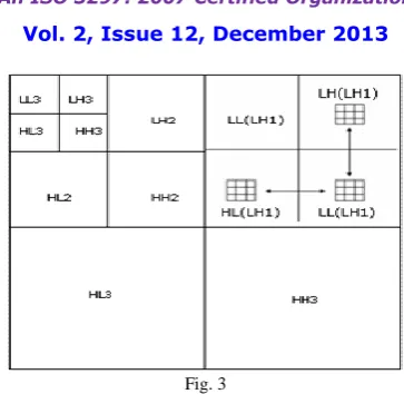
In the earlier method, we were decomposing only the coarse part. There exists the possibility to decompose the details part; we will also decompose the details part. In the above mentioned approach thresholding has been done locally in the particular sub-band only.
The original image at particular point is distributed in each sub band .While applying thresholding in particular window in a sub band, we do not consider any window in other sub band .But, there would be a corresponding window in other sub band, which would be correlated to the signal in the parent sub band and would also contain the information of image at the particular point. So, we have used the correlation property and applied the threshold limits for adaptively denoising the image.
As we can see from figure 5.1, the wavelet coefficients in each sub-bands of same level are determined using all three sub-bands of the same level. If estimated variance of coefficient Y(k) is less than the variance of the noise, σ2n ,then
that coefficients of X(k) are made zero assuming that this neighbourhood corresponds to noise .It is also possible that this point corresponds to edge information of the image .If estimated variance of Y(k) of that neighbourhood in other sub-band is much higher than σ2n , then it is more probable that this point corresponds to an edge .So, X(k) which have
made zero earlier , should be retained . Hence, it also preserves the edge. For determining neighborhood, we can choose different sizes of windows like 3*3, 5*5 .
Fig.2
Fig. 3
A.Denoising Procedure:
1) Apply three level decomposition at the image.
2)So, we have 10 sub-band LL3 ,LH3,HL3,HH3 ,LH2,HL2,HH2 , LH1,HL1,HH1 3) Reconstruct LL3 directly without any thresholding.
4) Pick LH1 and apply first level decomposition on it giving LL (LH1), LH (LH1), HL (LH1) & HH (LH1).
5) Then threshold LH(LH1), HL(LH1) HH(LH1) using our proposed approach .
6) Then reconstruct LH1 from LL(LH1) and thresholded LH(LH1), HL(LH1) HH(LH1) . 7) Repeat step 4,5,6 for each sub-band except LL3
VIII.RESULTS
Table1.Comparison of PSNR in Decibels for differentDenoisingMethods for Lena image.
σ =15dB σ =20dB σ =25dB VisuShrink 26.1618 26.7804 24.7053 Bayes Shrink 31.5612 28.6237 27.0705 MMSE 31.5737 28.9857 26.5383 Modified
Stochastic Method (Our Method) (3*3)
31.9618 30.3393 27.2638
Modified
StochasticMethod (Our Method ) (5*5)
31.9671 30.4844 27.4091
Table2. Comparison of PSNR in Decibels for differentDenoisingMethod for Barbara image.
σ =15dB σ =20dB σ =25dB Bayes
Shrink
32.6727 30.0467 27.1685 MMSE 32.0784 28.5889 26.1240 Modified
Stochastic Method (Our Method) (3*3)
33.1824 31.3024 28.8101
Modified Stochastic Method(Our Method) (5*5)
33.2177 31.6694 28.8408
a) b) c)
d)
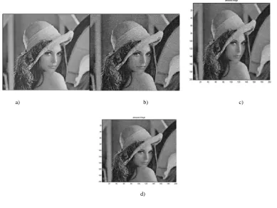
Fig. 4 a) Original b) Fig. 5 Noisy image (σ =20dB) c) .Denoised image (σ =20dB) , PSNR =28.99dB,MMSE Method
d) Denoised image (σ =20dB) ,PSNR =30.34dB, Modified stochastic Method(Our Method)
d)
Fig.5 a) Original image b) Noisy image (σ =25dB) c) Denoised image (σ =25dB) ,PSNR =26.5383 dB, MMSE Method d) Denoised image (σ =25dB) ,PSNR =27.26dB,Modified stochastic Method (Our Method)
IX.CONCLUSION AND DISCUSSION
In this paper we compared the various denoising techniques. We looked into the existing techniques like Visu Shrink; Bayes Shrink & MMSE based estimation techniques. We have seen that Visu Shrink is non-adaptive and uses universal threshold which would result in blurring of the images.. Thus, Bayes Shrink and MMSE based estimation has been used for better denoising of images. But, we are still missing some part of signals in the detail coefficients in these methods. So, if we could apply the thresholding adaptively on detail part, we would get better result. We can make it more adaptive by choosing different threshold values in a sub band. Basics of denoising involve operating around choosing the appropriate thresholds. Our approach modified stochastic method differs from the existing techniques, as has been showed by our results.
In our proposed method, band corresponding to detail coefficients were also decomposed to utilize the informationpresent in the details part. The decompositions were followed by determination of the threshold limit in each sub band .This made the threshold limit to be chosen adaptively and causes better denoising.
The results have shown that there has been considerable improvement in terms of Peak signal to noise ratio (PSNR) in comparison with other techniques.
Our Modified stochastic model uses correlation properties of signal in each sub-band and thus makes proper determination of an edge and noise in the image. Thus, this results in edge preservation in the image and retention of the good visual quality of the images.We have considered orthogonal wavelet for analysing the characteristics of the signal. If instead, we could use non orthogonal or semi orthogonal wavelets for analysing, the coefficients obtained would be more correlated and could give still better denoising techniques.
REFERENCES
[1] B. Widrow, J. R. Tlover, J. M. Cool, J. Kaunitz, C. S. Williams, R. H. Hearn, J. R. Zeidler, E. Dong,Jr., R. C. Goodlin, “Adaptive Noise Canceling Principles and Applications," Proceedings of the IEEE, vol. 63, pp. 1692{1716, December1975)
.
[2] Y. C. Lim and C. C. Ko, “Forward-Backward LMS Adaptive Line Enhancer,"IEEE Trans. Circuits Syst., vol. 37, no. 7, pp. 936{940, July 1990.
[3] N. J. Bershad and O. Macchi, “Adaptive recovery of a chirped sinusoid in noise, Performance of the LMS algorithm,” IEEE Trans. Signal Processing, vol. 39, pp. 595–602,Mar. 1991
.
[4] Donoho, D. L., “De-noising by soft-thresholding”, IEEE Trans. Info. Theory, vol. 41, pp. 613-627,May 1995 .
[6] S. Mallat, “A theory for multi-resolution signal decomposition: The wavelet reconstruction IEEE Trans. Pattern Anal. Machine Intell., vol. 11, pp. 674–693, July 1989.
[7] Martin Vetterli S Grace Chang, Bin Yu. Adaptive wavelet thresholding for image denoising and compression. IEEE Transactions on Image Processing, 9(9):1532-1546, Sep 2000.
[8] S. G. Chang, B. Yu, and M. Vetterli, “Spatially adaptive wavelet thresholding with context modeling for image denoising,” IEEE Transactions on Image Processing,. Aug 1998
[9]. R. W. Buccigrossi, and E. P. Simoncelli, “Image compression via joint statistical characterization in the wavelet domain”, IEEE Image Process., Vol. 8, No 12, Dec.1999, pp. 1688-1701.
[10]. J. K. Romberg, H. Choi, and R. G. Baraniuk, “Bayesian tree-structured image modeling using wavelet-domain hidden Markov models”, IEEE Image Process., Vol. 10, No 7, Jul. 2001,pp. 1056-1068.
.
[11] Marteen Jansen, Ph.D. Thesis in “Wavelet thresholding and noise reduction” 2000.
[12] M. Lang, H. Guo, J.E. Odegard, and C.S. Burrus, "Nonlinear processing of a shift invariant DWT for noise reduction," SPIE, Mathematical Imaging: Wavelet applications for Dual Use, April 1995.
[13] I. Cohen, S. Raz and D. Malah, “Translation invariant denoising using the minimum description length criterion”, Signal Processing, 75, 3, 201-223, (1999).
[14] T. D. Bui and G. Y. Chen, "Translation-invariant denoising using multiwavelets", IEEE Transactions on Signal Processing, Vol.46, No.12, pp.3414- 3420, 1998.