Design and Implementation of Linear Algebraic Controller for Broom Balancing

Design and Implementation of Linear Algebraic

Controller for Broom Balancing

Endalew Ayenew1, Dr. Sateesh Sukhavasi2

Sr. Lecturer, Dept. of Electrical Power & Control Engineering, Adama Science & Technology University,

Adama, Ethiopia 1

Associate Professor, Dept. of Electrical Power & Control Engineering, Adama Science & Technology University,

Adama, Ethiopia2.

ABSTRACT: This paper discusses how the broom isdynamically stabilizable. It is suggested because; the dynamics of the Broom is analogous to the dynamics of Pitch and Yaw motion of a rocket, and robot arm motion. The broom is mounted on a moving cart. The nonlinear dynamics of the system is modeled and linearized. For the linearized unstable system, Linear Algebraic Controller is designed to balance the broom, and the simulation result shows that the broom is well balanced even when it is initially disturbed to ±200 angles.

KEYWORDS: Broom Balancing, Unstable Non-linearity, Cart and Broom motions, Broom Angular Position.

I.INTRODUCTION

Children try to balance a long slim wood and broom (which is used to clean floor) on their palm or index finger. With the broom exactly centered above motionless hand, and nothing pushes it to one side; it was balanced. At equilibrium, it can stay that way indefinitely, but in practice it never does. The slightest shift of the broom's center of gravity to one side causes unbalance. Any disturbance that shifts the broom away from equilibrium gives rise to forces that push the broom still farther from equilibrium, so it becomes unstable. Any object that has no base of supporthas an unstable equilibrium and tips over when disturbed. Instability stems from the fact that its center of gravity always descends when it is tipped and it releases gravitational potential energy as a result. The broom is unstable in motionless hand. But if the hand is moved, the broom can be stabilized. This will be done by endlessly moving the hand under the broom's center of gravity. If the broom starts to tip to the left, its handle could be moved to the left to place the handle under the broom's shifted center of gravity, i.e. it needs to constantly adjust the position of the hand to keep the broom upright. In that manner, the broom is kept returning to its equilibrium. Even though the equilibrium is naturally unstable, it can be kept up by helping it out and make it dynamically stable.

The Broom Balancing (installedon a cart) does basically the same thing. But, to simplify the problem, it can be required to move in one direction.It is a well-known example of nonlinear unstable control problem. The naturally unstable equilibrium corresponds to a state in which the broom points strictly upwards and, thus, requires a control force to maintain this position. The basic control objective of the broom problem is to maintain the forced stable equilibrium position when the broom initially starts atsome angle.

II. LITERATURE SURVEY

missile guidance for military purpose, autopilot control (pitch, roll and yaw) of any air planfor stability (level flight) [16].Model of a Human Standing Still andinMusic instrument- Metronometo correct music rhythm.

In this paper, system setup for broom balancing generally includes the mechanical and electrical parts. The primary mechanical considerations are the cart and its propulsion, and the behavior of the broom. The electrical part of system setup includes sensor, signal amplifier, controller and motor drive circuits as shown in Fig.1.

Fig.1. Setup for Broom Balancing

III.METHOD

When the broom is at unstable position, it has two motions. First, the broom falls to its naturally stable equilibrium (down) position, i.e. leading motion- motion of center of gravity (cg) of broom with respect to a cart. The second is motion of the cart and the broom with respect to around. The broom moves with the cart when the cart moves to keep the broom at upright position due to leading motion.

Dynamic Model of the Broom:

Acronyms

G = gravitational acceleration

gc = broom gravity center

PP = pivot point

Xgc = X coordinate of broom gravity center

gc

Y

p

X

P

Y

H

F

V

F

l

m = broom mass

M = Total mass of the system



Br = Viscous damping constant at pivot point of broom

I =ml2/3: Moment of inertia for uniform rod of broom

Va = motor armature voltage

E = motor armature Emf

Td = motor developed torque

F = force applied to cart

φ = motor shaft angle

r = pulley’s effective radius

Km = voltage and torque constant of motor

Bm = motor viscous damping

ωm = motor angular speed ( m Xpp/r

 

 )

Bc = cart viscous damping

Jm = motor inertia

Mc = cart’s mass (M-m)

J = combined inertia of motor and cart (JJmMr2)

B = combined viscous damping of motor and cart

=

a m a m a

cr R B R K JR

B )/

( 2 2

 

Kc = viscous damping constant = kmr RaJ

For the whole system mathematical model determination, system seen in Fig.1 is divided in to two as shown in Fig.2 and Fig.3.Components of forces applied on the broom are shown in figure Fig.2.

Fig2.Diagram shows components of forces exerted on broom

Coordinates of point cg of the broom in terms of half of its length

l

= + cos

(2.1)

= + sin

(2.2)

Equation of Components of Forces applied on the Broom: When the downward-directed gravitation force and the opposing upward-directed force provided by pivot are not aligned, their resultant causes the application of a torque that tilts the broom. The magnitude of the torque increases as the angle of the falling broom increases relative to vertical axis.

1. Sum of forces in X direction:

∑ = ̈

(2.3)

= ̈ + ̈ − sin ̇

(2.4)

2. Sum of forces in Y direction:

∑ = ̈

(2.5)

= ̈ − cos ̇ +

3. Sum of moments about gravity center:

∑ = ̈+ ̇ (2.7)

sin − = ̈+ ̇ (2.8)

Substitute equations (2.4) and (2.6) into (2.8), we have

( + ) ̈+ ̇ − = − ̈ (2.9)

This is equation for the motion of abroom pivoted on the cart, which relatesthe cart and thebroom positions.

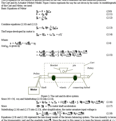
The Cart and its Actuator (Motor) Model: Figure 3 below represents the way the cart driven by the motor. In modelingmotion of the Cart and Motor, we need

Basic Equations of Motor

= + (210)

= ̇ (2.11)

= (2.12)

Combine equations (2.10) and (2.12)

= ̇+ (2.13)

TheTorque developed by motor is

= + + (2.14)

Where

= ̈ + ̇ + (2.4)

And is given by

= ̈ + ̇ + ( ̈ + cos ̈ − sin ̇

= ̈ + ̇ + (cos ̈ − sin ̇ ) (2.15)

Figure 3. The cart and its drive system Since M = Mc +m, and Substituting (2.15) into (2.14),

= + + ( ̈ + ̇ + cos ̈ − sin ̇ ) (2.16)

Since ̈ = ̇ = ̈ is motor shaft acceleration (2.17)

Substituting (2.16) and (2.17) into (2.13), after simplification, the motor armature input voltage is

= [ ̈ + ̇ cos ̈ − sin ̇ ] (2.18)

Equations (2.9) and (2.18) represent the non-linear model of the broom balancing system. The non-linearity is because of the trigonometric part and the quadratic term ̇ . Since the goal in this paper is to keep the broom upright at 0

0

 

that ̇will kept small so that its square is almost zero. Using this approximation the linearized dynamic model of the system is given by equations (2.19) and (2.21)

= [ ̈ + ̇ − ∅̈] - (2.19)

This equation relates the electrical variable-motor armature input voltage directly to thenon-electrical variables-cart and the broom positions.

For = simplification of equation (2.9) is

∅̈+ ∅̇ − ∅= ̈ (2.20)

Let 2 = , = , = ; ℎ

∅̈+ 2 ∅̇ − ∅= ̈ (2.21)

2.3 Determination of Transfer Functions ofthe System

From equation (2.19), solving forXpp ..

we have:

̈ _{= −} ̇ _{+ ∅̈ (2.22)}

Substitute (2.22) into (2.21) and solve for∅̈:

∅̈= ̇ + ∅ − ∅̇+ (2.23)

If we substitute (2.23) into (2.22),Xpp ..

will be obtained as:

̈ ₌ ̇ _{+ ∅ − ∅̇+ (2.24)}

Taking Laplace transform of equation (2.21), the transferfunction between X_pp(s) and (s)can be obtained as

∅ ( ) =

∅( )

( )= (2.25)

Also the Laplace transform of equation (2.24) is

( ) = ( )∅( ) ( ) (2.26)

Multiplying equation (2.25) and (2.26), and solving for

) (

) (

s V

s

a

 _{; after simplification we have:}

∅( ) =

∅( ) ( )=

( )

(2.27)

Fig4. Block diagram for closed loop transfer function of the system

Determination of the Parameters for the Broom Balancing System: To determine the stability of the broom, the parameters of the overall system are required. The parameters of the system such as mass of the cart- M, mass of the broom- m, length of the broom- L, radius of the pulley- r and motor armature resistance- Ra are all measured directly.

The motor constant parameter- Km was determined experimentally. The values of required parameters are listed in

table1.

Table 1: Parameters for the broom balancing System

Parameter Description Values M Total mass of the system 1kg

M Mass of rod 0.1kg

L Length of rod 0.5m

ℓ Length of rod from bottom to its centroid

0.25m

r Pulley radius 15mm

Bc Viscous damping of the cart

0.1N sec/m

Br Viscous damping at pivot point of broom

0.05Nm sec/rad

G Gravitation acceleration 9.8m/sec2

Km Motor constant for both torque and voltage

0.01Nm/A

Jm Motor inertia 0.01Nm sec2/rad

Bm Motor viscous damping 0.1Nm sec/rad

Ra Motor armature resistor 1

Inserting the parameter values in the table 1 into equation (2.27) the open-loop transfer functionrelating the broom angular position and required motor armature voltageis obtained as follows.

∅

( ) =

( )

=

.

.

As it will be seen in the next section, the dynamic equation ofbroom is unstable.Using Matlab, the pole-zero map and step response of the linearized model of broom (in open loop configuration) are shown in figure 5& 6 respectively, which indicatethe broom is unstable/ unbalanced.The step response of the uncontrolled closed-loop with unity feedback is shown in the Fig7. The response is almost identical with the open-loop step response. This indicates the system cannot be stabilized by simple unity feedback.

Fig5. Poles and zeroes map of open loop transfer function GΦ Fig6. Step response of the open-loop transfer function GΦ(s).

Reshaping of the system the response is necessary by incorporating proper controller in to the system to shift the unstable pole into the left half plane (stable region) of the s-plane.

Fig7. Step response for closed-loop uncontrolled broom balancing system with unity feedback.

IV. CONTROLLER DESIGN

First a desired closed loop transfer function- G0(s) is determined, and then solved for required controller. That is why it is called a linear algebraic method for controller design. It tries to satisfy a total prescribed system transfer function for single-input - single-output (SISO) systems.

For a plant with a proper transfer function ∅( ) =

( )

( ), with N(s) and D(s) coprime; and the transfer function ∅( ) =

( )

( )=

∅( )

( )meets the design specifications, where Vref(s)and ф(s) are reference input and output of closed-loop

system, respectively. The desired closed-loop transfer function G₀(s) is implementable if:

a) Degree of Do(s) minus degree of No(s)  degree of D(s) minus degree of N(s).

b) All closed loop right hand plan zeros of N(s) are retained in No(s).

Fig. 8Block diagram of unity feedback control system

The simpler attemptforapplication of the Linear Algebraic Method to determine controller transfer function Gc(s) with a

unity feedback system, the overall desired closed-loop transfer function in Fig. 8 is representedas

( ) = ∅( ) ( )= ( ) ( )= ( ) _∅( ) ( ) _∅( )= ( ) ( )

( ) ( ) ( )( ) ( ) (3.1)

For the unity feedback arrangement, for ∅( ), ( ) ( ) are as defined above and with degree of

( )≤degree of D(s)= n, from equation (3.1), we have

( ) ( ) + ( ) ( ) = ( ) (3.2)

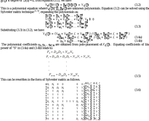
This is a polynomial equation where ( ) ( )are unknown polynomials. Equation (3.2) can be solved using the Sylvester matrix technique [1, 6], expanding the polynomials as;

( ) = + +. . . +

( ) = + +. . . + ; ≠0

( ) = + +. . . +

( ) = + +. . . + (3.3)

Substituting (3.3) in (3.2), we have

( ) = ( + +⋯+ )∗( + +⋯+ )

+( + +⋯+ ∗( + +⋯+ ) (3.4a)

= + +. . . + (3.4b)

The polynomial coefficients , … are obtained from pole-placement of ( ). Equating coefficients of like power of “S" in (3.4a) and (3.4b) leads to:

(3.5) This can be rewritten in the form of Sylvester matrix as follows.

                                                                       n n n n n n N D N D N D N D N D N D N D N D N D 0 0 0 0 0 0 0 0 0 0 0 0 0 0 1 1 0 0 1 1 0 0 1 1 0 0                                        cm cm c c c c N D N D N D 1 1 0 0 =                                           m n F F F 1 0 (3.6)

Equation (3.6) has solution if the matrix of coefficients has full row rank. In other wards the following condition hold true.

To achieve arbitrary pole-placement, the degree of controller Gc(s) in the unity feedback configuration must be m = n-1

or higher. If it is less than n-1, it may be possible to assign some of the poles but not all. The degree of the characteristic equation D₀(s) of transfer function G0(s) is + . The unknowns in (3.2) can be determined by (3.6) so

that for specified performance and coefficients, Gc(s) isexpressed as:

( ) = ( )

( )=

...

... (3.8)

For the stabilization of the system, the closed-loop poles of the transfer function G0(s) must be in the left hand side of

s-plane. The dominant poles of characteristic equation of G0(s) in the complex root plane approximately determine

transient performance and stability of a linear time invariant system. The damping ratio and the natural frequency resulting from the dominant poles of a more than two order system can be used to determine the boundary of a desired region in the complex plane within which all the roots of characteristic equation must be located. Assuming that dominant poles are complex roots and given as:

, =− ± (3.9)

Where is damping ratio

is un-damped natural frequency

= (1− )is damped frequency

We have to design a controller so that the step response of the closed-loop system meets the settling time (TS),delay

time (Td), maximum overshoot (Mp), damping ratio and steady-state error specifications [3]. The settling time and delay

timeare measures of the speed of the system response. Increasing the natural frequency- can increase the speed of the response. In general, the maximum overshoot decreases as the damping ratio increases. However, as damping ratio increases, the delay time increases which causes the response of the system sluggish. Therefore, suitable value of damping ratio should be selected to minimize the overshoot without affecting the speed of response of the system. To calculate dominant poles, let = 0.85 and Ts= 0.80 Sec

=

. = 5 = 5.88 / = 3.10 / = 0.63% <

10%

Using arbitrary pole-placement with unity feedback, the controller to stabilize the broom is designed next. From (2.28), the unstable pant transfer function is

∅( ) =

∅( ) ( )=

.

. =

( )

( ) (3.11a)

The numerator and denominator polynomials of G(s) can be written as:

( ) = 0 + 0 + 0.0579 + 0 (3.11b)

( ) = + 15.67 −60 −1136 (3.11c)

The order of the plant transfer function is n=3, and it needs controller Gc(s) of the order m = n-1 = 2. This shows the

degree of the characteristic equation D0(s) of the overall transfer function G0(s) is + = 5. Based on the

performance specifications setting taken above, the dominant poles are

, = ± = −5 ± 3.1

And the others arbitrary stable poles are selected as , =−16 ± 9 =−2, then polynomial of the

characteristic equation D0(s) is

= ( + 5 + 3.1)( + 5− 3.1)( + 16 + 9)( + 16− 9)( + 2)

= + 44 + 785.75 + 6420.83 + 27122 + 341767

= + +. . . + (3.11d)

Putting equations (3.11b) to (3.11d) in the matrix form to determine the unknown coefficients of polynomials Nc(s) and

                          0 1 0 0 0 0 0 67 . 15 0 1 0 0 058 . 0 60 0 67 . 15 0 1 0 1136 058 . 0 60 0 67 . 15 0 0 0 1136 058 . 0 60 0 0 0 0 0 1136                     2 2 1 1 0 0 c c c c c c N D N D N D =                     1 44 75 . 785 83 . 6420 33 . 27122 76 . 34174 (3.12)

X Y F

The unknown coefficients are determined using matlab command Y = inv(X)*F.

i.e. Y =

                    2 2 1 1 0 0 c c c c c c N D N D N D =                      7460 1 53 . 168013 33 . 28 62 . 993098 08 . 30 (3.13)

Therefore the desired closed loop and controller transfer functions are:

( ) =

. . (3.14)

( ) = . .

. . =

( )

( ) (3.15)

Where U(s) and E(s) are control and error signals as indicated in Fig.8 and (3.15) can be rewritten as: [-30.08s-2 +28.33s-1+1]U(s)

= [993098.63s-2 +168013.53s-1+7460] E(s) (3.16) If like power of s are collected together we get

U(s) = s-2[30.08 U(s) + 993098.63 E(s)] + s-1[-28.33 U(s) +168013.53 E(s)] + 7460 E(s)(3.17)this can be realized as Fig.9. Its synthesized practical circuit is a part of total circuit, which is used to stabilize the broom.

Fig.9Direct form realization of controller Gc(s)

V.RESULT AND DISCUSSION

The simulation result for step response of G0(s) is given by Fig.10. From the plot we get the following result.

The overall system is stabilized.

The control design meets performance specifications

 Maximum (peak) value =1.24 and settling time-Ts= 2.21sec due to arbitrary pole placement.

Using algebraic technique discussed above, the stability of the broom can be satisfactorily achieved by selection of arbitrary stable poles of overall transfer function of the system. And the performance specifications (large peak value and large settling time) of the overall system can be improved by proper selection of the poles.

Fig. 10Stabilized broom angle step response.

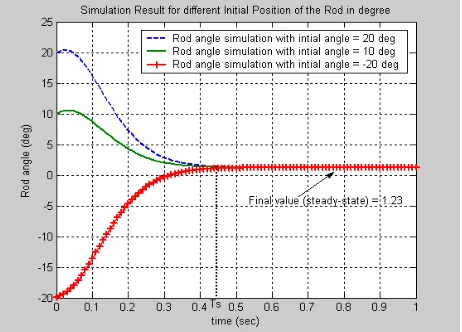
From equation (3.14), the current angular position of the broom is expressed in s-domain in terms of its initial

value-) 0 (

 (from vertical axis)and reference input voltage- Vref(s) and it is used to simulate effect of different values of (0)

on the stabilized system as shown in Fig.11.

∅( ) = ∅( ) ( ) ( )

. . (4.1)

The simulation result of step response of angular position of the broom for different values of initial angle (0)10, 20 and -20 (in degree) introduced between vertical axis and broom is shown below. From this plot, it is observed that the error or initial displacement angle of broom goes to some small final value (1.230) which indicates the broom returns to its balance (upright) position.

Fig.11Step response of broom angular position for different its initial angle

The frequency response simulation result for the combined transfer function of the plant and controller (G(s)Gc(s))is

Fig.12 Frequency response simulation result

Practically the controller is feasible. The controller given in Fig.9, sensor and motor drive parts are practically realized in Fig.13. The controller is ringed from resistances and operational amplifiers. During practical test, the result shows the broom is satisfactorily stabilized; and somewhat amplifier saturation is seen.

Fig.13 Complete circuit (controller, sensor and motor drive) realization

VI.CONCLUSION

that's why proper stabilizer is designed. The controller design methods are based on the transfer function approaches. The controllersatisfies both the stability of the system and design performance specification settings. Also the simulation result shows that for ±200-initial angle of the broom, the system is stabilized by the controllerwith in o.5 second and steady state value of 0.02rad (1.23 deg) for the broom is initially released from near ±200. This is due to for small deviation in broom angle; the sensor output is almost not changed. For the broom is at upright position, the output of controller is zero. In this case the controller does not get biasing signal. Broom Balancing provides a chance of designing a controller for a system that has good dynamic behavior. Hence the consideration for the transient response is emphasized. Another important point is that the broom on the cart provides a means for learning about electromechanical system.

VII. ACKNOWLEDGEMENTS

We thank God for the wisdom and perseverance that He has bestowed during this work and throughout our life.Also wewould like to acknowledge AdamaScience &Technology University, its staffs and our family members for their cooperation.

REFERENCES

1. B. Shawlan and M. Hassul“Control System Design-using Matlab” Prentice-Hall, 1980. 2. Nisit K. De and Parasanta K. Sen, “Electric Drives” Prentice-Hall, New Delhi, 2001.

3. Robert J. Schilling “Fundamentals of Robotics –Analysis and Control”, Prentice-Hall, New Delhi, 2000. 4. Thomas Kailalh , “Linear Systems”, Prentice-Hall, USA, 1980.

5. H. Kwarkernaak and R. Sivan, Wiley, “Linear Optimal Control Systems”,USA, 1972. 6. Chi-Tsong Chen, “Linear Systems Theory and Design”, CBS College, USA, 1984. 7. K. Ogata, Prentice-Hall, “Modern Control Engineering”, USA, 4thed, 2002. 8. Dorf and Bishop, Addison-Wesley, “Modern Control System”, 7thed, 1995. 9. M. Gopal, Wiley, “Modern Control System Theory”, New Delhi, 2nd_{ed, 1993.}

10. Erwin Kreyszig, “Advanced Engineering Mathematics”, Wiley, 8th_{ed, 1999.}

11. Benjamin C. Kuo, “Automatic Control Systems“, Prentice-Hall, 4th_{ed, 1982.}

12. David Pardoe, Michael Ryoo, and RistoMiikkulainen, "Evolving neural network ensembles for control problems," Proceedings of the 2005 conference on Genetic and evolutionary computation, Washington DC, USA, pp. 1379-1384 , 2005.

13. V.V. Tolat and B. Widrow, "An adaptive 'broom balancer' with visual inputs," IEEE International Conference on Neural Networks, pp. 641-647, 1988.

14. Carter, De Rubis, Guiterrez, Schoellig, Stolar. “Gyroscopically Balanced Monorail System Final Report” (2005) Columbia University. 15. ShlomoGeva and Joaquin Sitte, A cartpole experiment benchmark for trainable controllers IEEE Control Systems Magazine, vol. 13, pp. 40-

51, 1993.