Minireview on diffraction

(1)

Minireview on diffraction

Gösta Gustafson1,a

1_{Dept. of Astronomy and Theoretical Physics, Lund University}

Sölvegatan 14A, 22362 Lund, Sweden

Abstract.A short review is presented on diﬀractive excitation in high energy collisions.

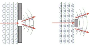
Figure 1.In optics a hole is equivalent to a black absorber.

1 Content

1. Optical analogy and Good–Walker formalism

2. Soft diﬀraction

• Reggeon theory

• QCD and the BFKL pomeron

3. Hard diﬀraction

2 Optical analogy and Good–Walker

In diﬀraction in optics, a hole is equivalent to a black ab-sorber, with a forward peak with an angular width θ ∼

λ/(opening width), see ﬁg. 1. Rescattering is described by a convolution in transverse momentum space, which corresponds to a product in transverse coordinate space. This implies that diﬀraction and rescattering is more eas-ily described in impact parameter space.

The optical theorem says that

ImAel=

1 2{|Ael|

2₊

j

|Aj|2}. (1)

Here the sum runs over all inelastic channelsj. For a struc-tureless projectile (e.g. a photon), diﬀraction corresponds to elastic scattering driven by absorption. If the absorption

a_{e-mail: [email protected]}

probability in Born approximation is given by 2F, then rescattering exponentiates inb-space, giving

dσinel/d2b=1−e−2F, (2)

and the optical theorem in eq. (1) gives:

ImAel =1−e−F (3)

dσel/d2b =(1−e−F)2 (4) dσtot/d2b =2(1−e−F). (5)

Diﬀractive excitation

As an example we can look at a photon in an optically active medium. Here righthanded and lefthanded photons move with different velocities, meaning that they propa-gate as particles with different mass. Study a beam of righthanded photons hitting a polarized target, which ab-sorbes photons polarized in thex-direction. The diff rac-tively scattered beam is then a mixture of right- and left-handed photons. If the rightleft-handed photons have lower mass, this means thatthe diffractive beam contains also photons excited to a state with higher mass.

Good–Walker formalism

For a projectile with a substracture, the mass eigen-states can differ from the eigenstates of diffraction. Call the diffractive eigenstatesΦn, with elastic scattering

am-plitudesTn. The mass eigenstatesΨkare linear

combina-tions of the statesΦn:

Ψk=

n

cknΦn (withΨin= Ψ1). (6)

The elastic scattering amplitude is given by

Ψ1|T|Ψ1=

c2₁_nTn=T, (7)

and the elastic cross section

dσel/d2b=(c2₁_nTn)2=T2. (8)

The amplitude for diﬀractive transition to the mass eigen-stateΨkis given by

Ψk|T|Ψ1=

n

cknTnc1n, (9) C

Owned by the authors, published by EDP Sciences, 2015

(2)

Figure 2.Ladder diagram related to pomeron exchange.

Figure 3.Mueller triple-Regge diagram. (Figure from ref. [1].)

which gives a total diﬀractive cross section (including elastic scattering)

dσdi f f/d2b=

k

Ψ1|T|ΨkΨk|T|Ψ1=T2. (10)

Consequently the cross section for diﬀractive excitation is

given by the ﬂuctuations:

dσdi f f ex/d2b=dσdi f f−dσel=T2 − T2. (11)

3 Soft diffraction

3.1 Reggeon theory

Pomeron exchange is described by a ladder exchanged be-tween the projectile and the target, as illustrated in ﬁg. 2. The elastic and total cross sections are given by

dσel/dt ∼(g2·sα(t)−1)2=g4s2(α(0)−1)e2(lns)α

_t

(12)

σtot ∼g2sα(0)−1 (13)

Note that α(0) > 1 implies thatσel > σtot for large s, which means that multi-pomeron exchange must be im-portant.

Inelastic diﬀraction is described by the Mueller triple-Regge formalism, illustrated in ﬁg. 3. The triple-pomeron contribution to the cross section is given by

σ∼g2

pP(t)gpP(0)g3P

⎛ ⎜⎜⎜⎜⎝ s

M2 X

⎞ ⎟⎟⎟⎟⎠2(α(t)−1)

M2_X(α(0)−1), (14)

whereg3Pdenotes the triple-pomeron coupling.

The triple (and multiple) pomeron couplings give loops, as illustrated in ﬁg. 4, which leads to complicated resummation schemes. The diagrams can also contain multipomeron vertices, see ﬁg. 5.

In particular three groups have studied these prob-lems: Tel Aviv (GLM) [2], Durham (KMR) [3], and Ostapchenko [4] (based on work by Kaidalov and cowork-ers). In this approach low-mass diﬀraction is included with the Good–Walker formalism, approximated by one excited state N∗, while high-mass diﬀraction is treated with the triple-regge formalism. At lower energies or excitations

Figure 4.Examples of pomeron loop diagrams (copied from the Tel-Aviv group).

Figure 5.Multi-pomeron vertices.Left: A cut through an event with diﬀractive excitation. Right: A vertex with coupling be-tweennandmpomerons.

also reggeons with α(0) ≈ 0.5 are included besides the pomeron. The regge intercepts and couplings are fitted to experimental data. We note here that these fits have been significantly modified after the presentation of the Totem data at 7 TeV, withσtot=98.6±2.2 mb andσel=25.4±1.1 mb [5].

• The Tel-Aviv group [2] has a single pomeron, with

αP(0)=1.23 andα≈0. This implies that the pomeron propagator is approximately a delta-function,δ(b), with no diﬀusion in b-space. Only 3-pomeron vertices are included.

• TheDurhamgroup [3] has in its new version from 2014

a single “eﬀective” pomeron with couplings dependent onk_⊥. It interpolates between a “bareIP" withαP(0)≈ 1.3 andαsmall, and a “softIP" withαP(0)≈0.08 and α ₌ ₀_._{25. Multi-pomeron couplings are large, with}

gn,m∝n mγn+m.

• Ostapchenko[4] has a formalism with two pomerons,

withαP(0)so f t =1.14 andαP(0)hard =1.31. The multi-pomeron couplings are ﬁxed by the relationgn,m∝γn+m, and thus not growing withnandmas fast as assumed by the Durham group.

The results obtained for the single diffractive cross sec-tion are presented in fig. 6, reproduced from Cartiglia [6]. The different experiments have different acceptance range inMX, and adjusting for this there is a general agreement between the results. We note in particular that Atlasand CMS have similar results, and also that these high energy results agree with tunes presented after the presentation of cross section data from Totem.

(3)

Figure 6.Single diﬀractive cross sections, compared with mod-els. Figure from ref. [6].

Figure 7. dσ/dηF _∼ _d_σ/_d_ln_M2

X. Data from Atlas[7] and model calculations from ref. [3].

dσ/dηF _∼ _d_σ/_d_ln_M2

X from KMR compared with data from Atlas.

3.2 QCD and the BFKL pomeron

Mueller’s dipole model

As mentioned above, unitarity constraints and satura-tion are much easier to account for in transverse coordi-nate space. Mueller’s dipole model [8, 9] is a formulation of LL BFKL evolution in impact parameter space. A color charge is always screened by an accompanying anticharge. A charge-anticharge pair can emit bremsstrahlung gluons in the same way as an electric dipole. The probability per unit rapidity for a dipole (r0,r1) to emit a gluon in the point

r2, is given by (cfﬁg. 8)

dP

dy =

¯

α

2πd

2_r 2

r2 01 r2

02r 2 12

. (15)

The important diﬀerence from electro-magnetism is that the emitted gluon carries away colour, which implies that the dipole splits in two dipoles. These dipoles can then emit further gluons in a cascade, producing a chain of dipoles as illustrated in ﬁg. 8.

Q

¯

Q

1

0

1

0

r01

2

r12

r02

1

0 2 3

y

x

Figure 8. A colour dipole cascade in transverse coordinate space. A dipole can radiate a gluon. The gluon carries away colour, which implies that the dipole is split in two dipoles, which in the largeNclimit radiate further gluons independently.

i j

2

1 3

4

Figure 9.In a collision between two dipole cascades, two dipoles can interact via gluon exchange. As the exchanged gluon carries colour, the two dipole chains become recoupled.

When two such chains, accelerated in opposite direc-tions, meet, they can interact via gluon exchange. This implies exchange of colour, and thus a reconnection of the chains as shown in ﬁg. 9. The elastic scattering amplitude for gluon exchange is in the Born approximation given by

fi j= α2

s 2 ln

2

r13r24 r14r23

. (16)

BFKL evolution is a stochastic process, and many sub-collisions may occur independently. Summing over all possible pairs gives the total Born amplitude

F=

i j

fi j. (17)

The uniterized amplitude becoms

T =1−e−fi j, ₍₁₈₎

and the cross sections

dσel/d2b=T2, dσtot/d2b=2T (19)

The Lund cascade model DIPSY

The DIPSY model [10–12] is a generalization of Mueller’s cascade, which includes a set of corrections:

• Important non-leading eﬀects in BFKL evolution. Most essential are those related to energy conservation and runningαs.

• Saturation from pomeron loops in the evolution. Dipoles with identical colours form colour quadrupoles, which give pomeron loops in the evolution. These are not included in Mueller’s model or in the BK equation.

(4)

e CMS

2

1 1

1 1 1 2

1 m σ 1 2 3 4 5 1 11 12 13 14

pp total cross sections

tot σ el σ fits tot σ est COM s 2 11. 1.5 ln s .134ln pp DG

DG p p D S

Figure 10.DIPSY results for total and elasticppcross sections, compared to experimental data.

1e-05 0.0001 0.001 0.01 0.1 1 10 100 1000 10000

0 0.5 1 1.5 2

-t (GeV2)

630GeV (x10) 546GeV (x100) 1.8TeV 14TeV (x0.1) UA4 Tevatron MC LHC

Figure 11. DIPSY results for the diﬀerential elasticpp cross section.

Figure 12.The virtual BFKL cascades are assumed to represent eigenstates for diﬀractive scattering. When they interact with a target, it can be absorbed in an inelastic event, give elastic scat-tering or diﬀractive excitation.

• The DIPSY MC gives also ﬂuctuations and correlations.

• It can be applied to collisions between electrons, pro-tons, and nuclei.

Some results forpptotal and elastic cross sections are shown in ﬁgs. 10, 11 [13]. (Here the initial proton wave function is approximated by three dipoles in a triangle.) We note that there is no input structure functions in the model; the gluon distributions are generated within the model.

Good–Walkervstriple–regge

It is natural to assume that the diﬀractive eigenstates for a colliding proton are the BFKL cascades, which can come on shell through interaction with the target, as illus-trated in ﬁg. 12,cfrefs. [14–17].

These diffractive states have a continuous distribution up to high masses, with large fluctuations. As demon-strated in ref. [18], calculating diffractive excitation via

proj.

target

y1

y2

Figure 13. Triple-pomeron diagram, withs=exp(y1+y2) and

M2

X =exp(y1).

the Good–Walker or the triple-regge formalism, is just dif-ferent formulations of the same phenomenon. An essential feature of the BFKL cascade is its stochastic nature. If the probability for a dipole split is given bydP/dy ∼λ, then the average number of dipoles, and the variance grow ac-cording to

n(y) ≈ eλy, (20)

V(y) ≡ n2₋_n2_≈_e2λy₋_eλy

= n2(1−e−λy). (21)

Thus the distribution satisﬁes approximate KNO scaling. For two colliding cascades, evolved to rapiditiesy1and y2respectively, we haves≈exp(y1+y2) =exp(Y), with Y ≡y1+y2. Assuming a dipole-dipole interaction

proba-bility 2f, we get for the bare pomeron exchange (neglect-ing unitarization eﬀects)

σinel∝eλy12f eλy2=2f eλY =2f sλ, (22) σel∝ f2e2λY= f2s2λ. (23)

This corresponds to a pomeron interceptα(0)=1+λ In the triple-reggeformalism, the triple-pomeron di-agram in ﬁg. 13 gives the following result for the inte-grated single diﬀractive cross section withM2

X <Mmax2 ≈ exp(y1):

(M<Mmax) dσS D

dlnM2dy1=f 2_e2λY

(1−e−λy1₎

= f2s2λ(1−1/(M_max2 )λ). (24)

In theGood–Walkerformalism this cross section is de-termined by the ﬂuctuations. For projectile excitation but intact target we obtain

σSD=T2targproj−Ttarg2proj= f

2_e2λY₍₁₋_e−λy1₎. ₍₂₅₎

We see that we get exactly the same expression in the two approaches. Most essential for this result is the approxi-mate KNO scaling.

(5)

10 100 1000

100 1000 10000

σ

(mb)

√s (GeV)

total elastic single diffractive

Figure 14. DIPSY result for cross sections before unitarization [17].

0.2 0.4 0.6 0.8 1 1.2 1.4 1.6

1 10 100 1000 10000

d

σSD

dlog(M

X

)

(mb)

M_X LHC 7 TeV

DISPY

Figure 15.Preliminary results from DIPSY fordσS D/dlnMXat 7 TeV.

as powers ofs, in accordance with a regge ﬁt with a single pomeron pole with parameters

α(0)=1.21, α=0.2 GeV−2 (26)

gpP(t)=(5.6 GeV−1)e1.9t (27) g3P(t)≈1GeV−1 (dep. on def.) (28)

We note also that when unitarization is omitted, the elastic cross section is larger than the total for √s>2 TeV.

Fig. 15 shows preliminary results fordσS D/dlnMXat 7 TeV, which should be compared with the LHC data in fig. 7. (Note that the diffractive mass grows in opposite directions in the two figures.)

4 Hard diffraction

Factorization and factorization breaking

UA8 at the CERN S ppS¯ collider (consisting of the UA2 central detector plus roman pots at 630 GeV) ob-served highp_⊥jets in diffractive events [19]. Jets have also been observed in gap events at HERA and the Tevatron. These events are often analyzed within the Ingelman– Schlein model [20], which assumes that the pomeron has a universal parton substructuref_qP,g(z,Q2). This implies that the diffractive cross section factorizes (cffig. 16):

σdi f f _∼ i

F_Pp(xP)⊗fiP(z=xB j/xP,Q2)⊗σˆγ∗i. (29)

Figure 16. A diagram for hard diﬀraction in the Ingelman– Schlein model.

Figure 17. Pomeron pdf:s determined by Zeus, together with a

comparison with data for the distribution in the observed parton fraction of the pomeron momentum,zobs

P [21].

HerexPis the energy fraction carried by the pomeron, and the sum runs over diﬀerent parton speciesi.

A fit with DGLAP evolution to HeraDIS data for hard and soft diffraction by Zeus[21] is shown in fig. 17, to-gether with a comparison with data for the distribution in the observed parton fraction of the pomeron momentum,

zobs

P . We note in particular that the distributions are gluon dominated. The Ingelman–Schlein model is implemented in a number of MC generators, e.g. POMPYT, Pythia8,

and POMWIG.

Factorization was proved by Collins for hard scatter-ing in DIS [22]. Results from the Tevatron showed, how-ever, that factorization is strongly broken when comparing diffractive two-jet events in DIS and pp collisions [23]. Inppscattering the gaps become frequently filled by soft interactions. Figure 18 shows the ratio between single diffractive and non-diffractive events (R =S D/ND) from CDF, which are a factor 0.1 – 0.2 below the correspond-ing DIS data. Similarly fig. 19 shows a fit to data for

dN/dξ˜ ≈dN/d(M2

X/s), where the pomeron ﬂux is renor-malized in the MC with a gap survival probability≈ 0.2 [24].

Similarities between diﬀractive and non-diﬀractive scattering

(6)

Figure 18.The ratioR=S D/ND. Data from CDF compared to expectation from NLO ﬁt to HERA data, assuming factorization [25].

Figure 19. Data ondN/dξ˜ ≈dN/d(M2

X/s) measured by CMS, compared with expectations with a pomeron ﬂux rescaled by a factor 0.2 [24].

E_⊥, for diffractive and non-diffractive events, which in-dicates that the same hard subprocess is at work. There is a gap survival probabilityS2_{, but}_{no extra suppression} ∼1/Q2_{for di}_ff_{ractive events}_{. This is consistent with}

Gou-lianos’ empirical “renormalized pomeron” [26], and also with the assertion that hard diﬀraction is leading twist by Kopeliovichet al.[27].

The gap survival probability for multiple gaps is diffi -cult to calculate. Some processes with multiple gaps are shown in fig. 21. CDF has studied the ratios 2-gap/ no-gap (SDD/SD) and one-gap/no-gap (DD/tot). The results, reproduced in fig. 22, show thatmultiple gaps are not mul-tiply suppressed. This feature is also consistent with Gou-lianos’ renormalized pomeron [26].

Central exclusive production

Many schemes are proposed for gap survival in central exclusive production (seee.g.refs. [31–34]).

Fig. 23 shows a diagram including eikonal and en-hanced survival factors from the Durham group. Gap

sur-Figure 20. The distribution of diﬀractive and non-diﬀractive two-jet eventsvsmeanE⊥, measured by CDF (from Goulianos, proc. 13th Blois Workshop, 2009 [28].)

Figure 21.Diﬀerent processes with multiple gaps. (Figure from Goulianos, proc. 13th Blois Workshop, 2009 [28].)

Figure 22. Ratios 2-gap/no-gap and one-gap/no-gap, compared to a regge prediction and the prediction from a renormalized pomeron [29].

vival factors have been determined from experimental data forQQ¯and two-jet production. As a rule of thumb they are approximately 0.2 – 0.3 at the Tevatron, reduced to∼0.03 at LHC.

Interesting processes for further studies include:

(7)

Figure 23.Diagram for hard central production from KMR, with eikonal and enhanced survival factors. (Figure from ref. [30].)

• Jet–gap–jet events in double diﬀraction, as a means to study BFKL evolution.

• Studyγγ→γγorγγ→W+W−, which can give infor-mation about possible anomalous weak couplings.

• Higgs search.

5 Conclusions

Soft diﬀraction

Several groups have presented analyses of elastic and diﬀractive cross sections within the Regge formalism. They can contain either one pomeron (GLM), a soft and a hard pomeron (Ostapchenko), or a pomeron interpolating between soft and hard (KMR). Unitarization is taken into account by summation of pomeron loop diagrams, where the results also depend on the assumptions made for multi-pomeron vertices, which vary between the groups. For lower masses,MX, contributions from low-lying reggeon trajectories are also important, and have to be included with extra parameters. The Regge-based formulations also generally include production of low massN∗ resonances within the Good–Walker formalism, approximating it with two or three diﬀractive eigenstates.

High mass diffraction has, however, also been de-scribed using the Good–Walker formalism. The dynam-ics of BFKL evolution implies large fluctuations, where the gluon multiplicity satisfies approximate KNO scal-ing. This implies that Good–Walker reproduces the regge form for diffractive excitation. Thus the triple-pomeron and Good–Walker formalisms actually describe the same

physics. The Good–Walker formalism can here have the

advantage that the results do not depend on new tunable parameters.

(When comparing theory with data, we note that at high energies, low mass diﬀraction is very diﬃcult to mea-sure experimentally, and its behaviour is therefore less well-known.)

Hard diﬀraction

Hard diﬀraction is commonly analyzed by means of the Ingelman–Schlein formalism, assuming a factorized form with a partonic structure for the pomeron. Factor-ization is, however, strongly broken when comparing data for ppandγpscattering, due to soft exchange in pp

re-actions. The survival probability in ppcollisions is esti-mated to∼0.1−0.2 at the Tevatron, and∼0.03 at LHC.

Data from the Tevatron indicate that the same hard subprocess is at work in diﬀractive and non-diﬀractive hard processes, and that multiple gaps are not multiply suppressed. These features are in agreementt with Gou-lianos’ empirical renormalized pomeron.

The LHC detectors have larger acceptance in rapidity than the detectors at Heraor the Tevatron, which implies that we can look forward to many interesting analyses us-ing roman pots at the LHC.

References

[1] E. Luna, V. Khoze, A. Martin, M. Ryskin, Eur.Phys.J.C59, 1 (2009),0807.4115

[2] E. Gotsman, E. Levin, U. Maor (2014),1403.4531 [3] V. Khoze, A. Martin, M. Ryskin (2014),1402.2778 [4] S. Ostapchenko, Phys.Rev. D83, 014018 (2011),

1010.1869

[5] G. Antchev et al. (TOTEM Collaboration), Euro-phys.Lett.101, 21002 (2013)

[6] N. Cartiglia (2013),1305.6131

[7] G. Aad et al. (ATLAS Collaboration), Eur.Phys.J. C72, 1926 (2012),1201.2808

[8] A.H. Mueller, Nucl.Phys.B415, 373 (1994)

[9] A.H. Mueller, B. Patel, Nucl.Phys. B425, 471 (1994),hep-ph/9403256

[10] E. Avsar, G. Gustafson, L. Lonnblad, JHEP 0507, 062 (2005),hep-ph/0503181

[11] E. Avsar, G. Gustafson, L. Lonnblad, JHEP 0701, 012 (2007),hep-ph/0610157

[12] C. Flensburg, G. Gustafson, L. Lonnblad, JHEP 1108, 103 (2011),1103.4321

[13] C. Flensburg, G. Gustafson, L. Lonnblad, Eur.Phys.J. C60, 233 (2009),0807.0325

[14] H.I. Miettinen, J. Pumplin, Phys.Rev. D18, 1696 (1978)

[15] Y. Hatta, E. Iancu, C. Marquet, G. Soyez, D. Triantafyllopoulos, Nucl.Phys.A773, 95 (2006),