A Comparative Analysis of Open Source Software Reliability

(1)

A Comparative Analysis of Open Source

Software Reliability

Cobra Rahmani, Azad Azadmanesh and Lotfollah Najjar College of Information Science & Technology

University of Nebraska-Omaha, U.S. E-mail: {crahmani, azad, lnajjar}@unomaha.edu

Abstract— The purpose of this study is to compare the

fitting (goodness-of-fit) and prediction capabilities of three reliability models using the failure data of five popular open source software (OSS) products. The failure data are modeled by Weibull and two other Non Homogenous Poisson Process (NHPP) models (Yamada S-Shaped and Schneidewind). The OSS products considered are Eclipse,

Apache HTTP Server 2, Firefox, MPlayer OS X, and ClamWin Free Antivirus. Weibull is chosen due to its

popularity in lifetime and its flexibility in modeling various distributions. On the other hand, among many software reliability models, the NHPP models are prevalent. The goodness-of-fit is based on the entire failure data collected. Prediction is accomplished by estimating the models parameters based on partial failure history and then applying the estimates to the entire time span for which failure data is collected. The outcomes show that a reliability model that fits the failure data well may not necessarily be a decent forecaster of future failure patterns.

Index Terms-- Software reliability growth model,

Non-homogeneous poisson process (NHPP), Open source software (OSS), Prequential likelihood ratio (PLR), Weibull distribution.

I. INTRODUCTION

Open Source Software (OSS) in general refers to any software whose source code is freely available for distribution. The success and benefits of OSS can be attributed to many factors such as code modification by any party as the needs arise, promotion of software reliability and quality due to peer review and collaboration among many volunteer programmers from different organizations, and the fact that the knowledge-base is not bound to a particular organization, which allows for faster development and the likelihood of the software to be available for different platforms. Eric Raymond in [1] states that “with enough eye balls, all bugs are shallow”, which suggests that there exists a positive relationship between the number of people involved, bug numbers, and software quality. Some examples of successful OSS products that are used in this paper are Apache HTTP server, Eclipse framework and the Mozilla Firefox internet browser.

For the purpose of this study, five different OSS products are selected: Eclipse, Apache HTTP Server 2,

Firefox, MPlayer OS X, and ClamWin Free Antivirus.

These projects are chosen because of their high number

of downloads, length of project operation, and sufficient number of bug reports. MPlayer OS X and ClamWin Free Antivirus are two projects, which can be found in sourceforge.net [2]. MPlayer OS X, launched in 2002, is a project based on MPlayer, which is a movie player for Linux with more than six million downloads. ClamWin Free Antivirus was launched in 2004 that has had more than 19 million downloads. Both of them use sourceforge.net as their online bug-repository. Eclipse, Apache 2, and Firefox are the other three OSS projects, which use Bugzilla [3] as their bug-repository system. Bugzilla is a popular bug-repository system that allows users to send information about a detected bug such as bug description, severity, and reporting time.

Additionally, these projects are well-known and have been in operation for more than four years. Therefore, there is a sufficient amount of failure data to provide a decent picture of software quality, which may otherwise lead to anomalous reliability estimates [4,5].

This study compares Weibull, S-shaped, and Schneidewind distribution models in terms of goodness-of-fit and reliability prediction based on the failure data collected for the selected OSS products. Weibull distribution is widely utilized in lifetime data analysis because of its flexibility in modeling different phases of bathtub reliability, i.e. decreasing, constant, and increasing failure rates. The function has been particularly valuable for situations for which the data samples are relatively small, such as in maintenance studies [6]. On the other hand, Non-Homogeneous Poisson Process (NHPP) has gained much popularity in the software reliability field. In general NHPP models are grouped into exponential and non-exponential models. To cover both groups, one model from each group is selected. S-shaped model is a non-exponential NHPP model [7]. Additionally, the per-fault distribution of S-shaped model follows the Gamma distribution [8], which is representative of failure patterns whose distributions are skewed. The S-shaped model reflects the fact that the cumulative number of failures is often S-shaped relative to the exponential curve. Among multiple reasons, it is believed that there is a learning curve during the testing phase of the software product. Initially, the testers are becoming familiar with the product and hence there is a slow increasing curvature in removing faults. As testers’ skills improve, the rate of uncovering defects

(2)

increases quickly and then levels off as the residual errors decreases sharply or become more difficult to detect.

On the other hand, if the duration for which the increase in failure intensity reaches a peak is short, before a decreasing pattern of failures is observed, an exponential NHPP might be able to model the failure pattern more accurately. This observation is also supported by [9]. For this reason, Schneidewind’s model which is an exponential model is selected and the failure intensity is assumed to be decreasing exponentially [10]. Schneidewind’s model has been recommended by IEEE Reliability Society [11] and the American Institute of Aeronautics and Astronautics (AIAA) [12] as one of the models to be attempted for initial fitting failure data. As reported by Lyu [13], Schneidewind’s model was used on IBM’s flight control software models with very good success [14].

The rest of the paper is organized as follows. Section II provides some definitions and background information. Section III concentrates on failure data analysis and comparison study of the selected models in terms of reliability estimates and reliability prediction. Section IV concludes the paper with a summary.

II. BACKGROUND

As software products have become increasingly complex, software reliability is a growing concern, which is defined as the probability of failure free operation of a computer program in a specified environment for a specified period of time [8,15]. Reliability growth modeling has been one approach to address software reliability concern, which dates back to early 1970’s [16, 17,18]. Reliability modeling enables the measurement and prediction of software behaviors such as Mean Time to Failure (MTTF), future product reliability, testing period, and planning for product release time.

Different classifications of software reliability models exist. One way is to categorize the models based on the deterministic and probabilistic nature of the parameters used [8]. The deterministic models do not involve random variables. They attempt to obtain performance measures by accounting for some software structure and attribute, such as logical complexity by counting the decision point in a program [19] and program length by the number of distinct operators and operands in the software [20]. On the other hand, a large number of models belong to the probabilistic category, which place probabilistic assumptions on the parameters of the models, such as failure occurrences [7,10,21,22,23]. One subcategory of probabilistic models is Non-Homogeneous Poisson Process (NHPP) models [24], which was originally studied in hardware reliability. These models assume that the failure process varies with time and the cumulative number of failures up to time t is Poisson distributed with a parameter that is the mean value of failures.

Another classification is to divide the software reliability models into time-domain and failure-domain models. The main input parameter to time-domain models is individual times of each failure. Some models

may require the intervals of successful operations, which can be obtained by subtracting each time of failure from the next failure time. As the failures occur and fixed, it is expected that these intervals to increase. Some examples that belong to this class of reliability modeling are Jelinski-Moranda and Littlewood models [17,25].

The failure-domain models labeled as such because the input parameter of study is the number of failures in a specified interval of time rather than successful operation intervals between failures. Normally, the failure intensity is used as the parameter of a Probability Distribution Function (PDF). Like the first class, as the fault counts drop, the reliability is expected to increase [8,26,27]. Examples of this class are Goel-Okumoto, S-shaped, and Musa-Okumoto models [7,15,21]. As it will be seen, the input to the Weibull model is time-domained, whereas S-shaped and Schneidewind models belong to the failure-domain category.

White-box and black-box models are two approaches for predication of software reliability. The white-box models attempt to measure the quality of a software system based on its structure that is normally architected during the specification and design of the product. Relationship of software components and their correlation are thus the focus for software reliability measurement [28,29,30,31]. In the black-box approach, the entire software system is treated as a single entity, thus ignoring software structures and components interdependencies. These models tend to measure and predict software quality in the later phases of software development, such as testing or operation phase. The models rely on the testing data collected over an observed time period. Some popular examples are: Yamada S-Shape, Littlewood-Verrall, Jelinski-Moranda, Musa-Okumoto, and Goel-Okumoto [7,15,21,25,32]. This study is concentrated on the black-box reliability approach to measure and compare the reliability of the selected OSS projects.

A. General Distribution Functions

A fault or bug is a defect in software that has the potential to cause the software to fail. An error is a measured value or condition that deviates from the correct state of software during operation. A failure is the inability of the software product to deliver one of its services. Therefore, a fault is the cause for an error, and software that has a bug may not encounter an error that leads to a failure. Failure behavior can be reflected in various ways such as Probability Density Function (PDF) and Cumulative Distribution Function (CDF). PDF, denoted as f(t), shows the relative concentration of data samples at different points of measurement scale, such that the area under the graph is unity. CDF, denoted as F(t), is another way to present the pattern of observed data under study. CDF describes the probability distribution of the random variable, T, i.e. the probability that the random variable T assumes a value less than or equal to the specified value t. In other words,

) ( ) ( ) ( ) ( ) (t PT t f x dx f t F' t F = ≤ =

∫

t ⇒ = ∞ −

(3)

Therefore, f(t) is the rate of change of F(t). If the random variable T denotes the failure time, F(t), or unreliability, is the probability that the system will fail by time t.

Weibull Distribution – The PDF of Weibull function is

β α β β α β (/ ) 1 ) (t t e t f − − = (1) where α is the scale parameter and β represents the shape parameter of the distribution. The effect of the scale parameter is to squeeze or stretch the distribution. The Weibull PDF is monotone decreasing, if 1. The smaller β, the more rapid the decrease is. It becomes bell shaped when β > 2, and the larger β, the steeper the bell shape will be. Furthermore, it becomes the Rayleigh distribution function when β = 2 and reduces to the exponential distribution function when β = 1. Fig. 1 shows the Weibull PDF for several values of the shape parameter when α = 1 [26].

Figure 1. Weibull PDF for several shape values when α =1. The mean function of Weibull, i.e. the expected number of failures in interval [0, t], is

(2) where N is the total number of failures in the software product. The failure rate at t, denoted as λ(t), which is the rate at which failures occur per interval, is

Schneidewind’s Model – This model assumes that the cumulative number of failures is NHPP. The model is built on the belief that the failure frequency changes over time and that the recent failures are more beneficial to predicting the future behavior than the past failures. Based on this, the model provides for three forms of failure models [11]. For instance, it allows for the early failure counts to be dropped if those failures are believed to contribute little to the future forecasts of failures. This study assumes that all failures are important and thus no failures are discarded.

The model assumes that the failures are independent. The mean value of failures is [11]:

1 (3) where α is the initial failure rate and β is the negative of derivative of failure rate. The model places an upper bound on the number of failures, i.e. lim / . The failure rate, is an exponentially decreasing function,

Therefore, a large (small) implies a small (large) failure rate, and the initial failure rate, i.e. the failure rate at t = 0 is .

S-shaped Model – Experience has shown that the cumulative number of faults is often S-shaped, rather than exponentially shaped. This means that the curve representing the cumulative number of faults shows a dip in the early part of the graph and then follows an exponential growth. The two common S-shaped NHPP models are the inflection and the delayed models. The latter, herein referred to as the S-shaped model is characterized by its S-shaped mean value m(t) [8],

( ) [1 (1 ) ] bt e bt a t m = − + − (4) where a denotes the number of faults in the software product and b is the failure rate in the steady state, also referred to as the constant of proportionality. The model assumes that the faults in the software product are independent of each other, and all detected faults are immediately removed without introducing any new fault.

Since the failure rate, , is the derivative of m(t), (5) If α_andβ are the scale and shape parameters, (5) is representative of the Gamma function with parameters α = 1/b and β = 2. In this function, the shape parameter 2 is indicative of skewed distribution, as shown in Fig. 1.

For each of the three models described, the estimated failure intensity during the time interval ℓ ,

, is

ℓ (6) where is the model’s estimated mean value of failures for the interval [0, ].

B. Prequential Likelihood Ratio (PLR)

The PLR function [33,34] compares predictions from two models based on the same data source in order to determine the model with the most likelihood accurate prediction. Given two models A and B and equal probability of prior belief for both models, the prequential likelihood values and of the models are computed for n predictions. If the ratio /

shows overall growth as n increases with the possibility of some fluctuations, then model A provides better prediction than model B [33].

More precisely, assume the prior observed failure intensities for ℓ, 1 . The prequential likelihood

is defined as follows 0 0 0.5 1 1.5 2 2.5 3 3.5 4 1 2 3 t β = 0.5 β = 1 β = 2 β = 4 β = 10 β = 0.5 β = 10 β = 1 _β_{= 2}β = 4 f(t)

(4)

ℓ

A comparison of predictions for the two models A and B can be found by the ratio of their as follows

.

Dawid in [33] shows that if ∞, as ∞, then model A is favored over model B.

III. EXPERIMENTAL ANALYSIS

Prior to analyzing the performance estimates of the reliability growth models, i.e. Weibull, S-shaped, and Schneidewind, the failure data for the five selected OSS products must first be collected and filtered. Therefore, the reliability estimate process is partitioned into three steps: bug-gathering, bug-filtering, and bug-analysis. In the bug-filtering step, the raw failure data from each software product is collected using an online bug-repository system. The online system is capable of archiving failure information reported by users who experience flaws or failure in the product. The quality of reliability estimation highly depends on sufficient error reports and the accuracy of reports provided by the users. Although, the bug reports may differ among software products, each bug report normally contains the appropriate fields to signify the following: 1) a unique identification value for the report, 2) the time/date the bug is reported, 3) some information about the user reporting the bug, 4) the product name, and 5) the status of the bug-report filled by the organization in charge of the product development, such as whether the bug is fixed, valid, deleted, or fixed. The duration for which the failure data is collected for the five OSS products is listed in Table I. As indicated, the bug-reports are collected from sourceforge.net and bugzilla.

TABLE I.

DURATIONS OF COLLECTED FAILURE DATA1

Project name Start date End date

Firefox 03/19992_10/2006

Eclipse 10/20013_12/2007

Apache 2 03/2002 12/2008

ClamWin Free Antivirus 03/2004 08/2008

MPlayer 09/2002 06/2006

During the bug-filtering step, the reports collected in the first step are filtered out to remove the unwanted reports. For example, some reports might be duplicates, not represent a real defect, or the information provided may not be complete. Among the bug-reports for MPlayer and ClamWin, those reports with status other than “Deleted” (not a valid report) are collected. The

1

The start date of collected bug reports is the earliest date wherein a bug is reported.

2_{The failure data collected prior to the official release date of Firefox} are obtained from Mozilla bug reports.

3_{This date is prior to the official release date.}

reports for the other three products, i.e. Eclipse, Apache, and Firefox, are initially in XML format. A Java program has been developed to gather the relevant data from the XML format of each report. The resultant bug-reports are then filtered out. Those bug-reports with the following status values are accepted and the rest are discarded: FIXED (bug is fixed), WONTFIX (bug will not be fixed), LATER (bug won’t be fixed in the current product version), and REMIND (bug probably won’t be fixed in the current product version).

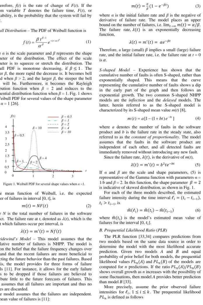
Finally, in the bug-analysis step, the dates of the filtered bug-reports are used to organize the reports into two-week intervals for further analysis. Fig. 2-64 exhibit the failure intensities for the five OSS products. The x-axis and y-x-axis represent each biweekly period and its corresponding failure intensity, respectively. Also, each graph shows the interval for which the failure reports are collected. For instance, x-axis in Fig. 2 contains 115 points, which is equivalent to about 4.4 years of collected failure data for ClamWin operation. The failure patterns of these graphs are used in the next section in terms of goodness-of-fit and failure forecasts (prediction) by the three models, i.e. Weibull, S-shaped, and Schneidewind models.

Figure 2. Filtered bug frequency for ClamWin Free Antivirus product.

Figure 3. Filtered bug frequency for MPlayer OS X product.

4

The intensities of bug reports are connected to form smoother plots. The purpose is to better visualize the pattern of failure reports.

0 4 8 12 16 20 1 21 41 61 81 101 Biweekly Time Failur e Intensity (FI ) 0 5 10 15 20 25 1 7 ₁₃ ₁₉ ₂₅ ₃₁ ₃₇ ₄₃ ₄₉ ₅₅ ₆₁ ₆₇ ₇₃ ₇₉ ₈₅ ₉₁ ₉₇ Biweekly Time Failur e Intensity (FI )

(5)

Figur Figu Figu A. Goodness Weibull Mod projects, i.e. Free Antivir represented b example, Fi superimposed pattern is sup that software by Rayleigh distribution considered a stabilizes at a In closed usually an in software to th 0 10 20 30 40 50 60 1 ₁₁ Failur e Intensity (FI ) 0 200 400 600 800 1000 1200 1400 1600 1800 1 ₁₀ Failur e Intensity (FI ) 0 10 20 30 40 50 60 70 80 90 100 1 6 Failur e Intensity (FI ) re 4. Filtered bug ure 5. Filtered bu ure 6. Filtered bu -of-fit Estima del - The bug Apache 2, M rus, appear to by the Weibu ig. 7 shows d on the bug pported by lar e projects follo h distribution with shape p a desirable pa

a very low lev source softw ndicator of end he field [26]. T 11 21 31 41 51 61 10 19 28 37 46 55 Biwe 6 ₁₁ ₁₆ ₂₁ ₂₆ B g frequency for Ap ug frequency for E ug frequency for F ate g frequencies MPlayer OS o follow a pa ull distribution this pattern frequencies f rge body of em ow a life cycle function, wh parameter β = attern since th vel.

ware, the stabi ding test effor This pattern is 61 71 81 91 101 111 Biweekly Time 64 73 82 91 ₁₀₀ eekly time 31 36 41 46 51 Biweekly Time pache 2 product. Eclipse product. Firefox product. for three of X, and Clam attern that ca n function. A n that is vis for Apache 2. mpirical studi e pattern desc hich is a We 2 = . This is he bug arrival ilizing behavi rt and releasin s also supporte 111 121 131 141 151 161 109 118 127 136 145 51 56 61 66 71 these mWin an be As an sually This ies in ribed eibull also l rate ior is ng the ed by Mus easil bugs exam rate cont F O follo bug the r the p simi Clam frequ in on in Fi R with anal frequ vers beca vers A mult lack repo Ther unif rates hind 161 171 154 76 Frequen cy Intensity (FI ) 1 1 1 1 1 Bu g Fr e q ue n cy sa-Okumoto m ly at the begin s tend to be mple, they are

of undetecte tinues [27]. Figure 7. A curve On a quick gla ow this patter reports includ reports for eac pattern of failu ilar pattern as mWin Free uencies for in ne diagram, in ig. 5. Figure 8. Filtered Rather than de h similar patte lyzed for relia uencies for E ion will be ause of its hi ions. A similar case tiple peaks in k the version n ort contains refore, differe fied version. A s seem not to ders the accura

0 10 20 30 40 50 60 1 ₁₁ ₂₁ ₃₁ 0 200 400 600 800 1000 1200 1400 1600 1800 1 7 _{13 19} ₂₅ _{31 37} ₄₃ model in that t nning of testin more difficu not exercised ed bugs drop

e fitted onto bug f ance at Fig. 5 rn. Further inv de failures abo ch version are ure intensities those of Apa Antivirus. Fi ndividual Ecli nstead of lum d bug frequencies different versio ealing with m erns, one sing ability estimat Eclipse V2.0 e used in relia igh bug repor

e could be tru Fig. 6. Howev numbers. The the phrase “ ent versions of Another observ have stabilize acy of reliabili 31 41 51 61 71 81 Biweekly Tim 43 49 55 61 67 73 79 85 91 97 Biweekly Time the simple bu ng phase and t ult to detect d frequently. T s exponential frequencies for A , Eclipse doe vestigation rev out multiple ve extracted, it i s for each vers ache 2, MPlay ig. 8 illustra ipse releases mping them in s of Eclipse produ ons. multiple versio gle version is tion. Fig. 9 sh extracted from ability analysi rts in compar ue for Firefo ver, the Firefo version field “Trunk” for f Firefox are t vation is that th ed at a low lev ity estimates. 81 91 ₁₀₁ ₁₁₁ ₁₂₁ ₁₃₁ me 97 _{103 109} _{115 121} ₁₂₇ _{133 139} ₁₄₅ ₁₅₁

ugs are caught the remaining because, for Therefore, the lly as testing Apache 2 product. s not seem to veals that the ersions. When is noticed that sion follows a yer OS X, and ates the bug superimposed one graph as

uct for

ons of Eclipse extracted and hows the bug m Fig. 8. This is of Eclipse rison to other ox because of ox bug reports of each bug-all versions. treated as one he bug arrival vel yet, which

131 141 151 161 171 157 Eclipse V2.0 Eclipse V2.1 Eclipse V3.0 Eclipse V3.1 Eclipse V3.2 Eclipse V3.3 t g r e g o e n t a d g d s e d g s e r f s -. e l h

(6)

Figure 9. Filtered bug frequencies for Eclipse V2.0 product. The R Project [35] is a freely available package that is used for a wide variety of statistical computing and graphics techniques. R is able to apply the Maximum Likelihood Estimation (MLE) technique [8] for estimating the parameters of Weibull distribution. Since R requires time-domain data, the relative frequency of bug reports needs to be converted to occurrence times of failure. Therefore, each bug report is mapped to its corresponding biweekly period. For example, 4 bugs reported in the 1st biweekly and 3 bugs reported in the 2nd biweekly periods are converted to: 1,1,1,1,2,2,2. This further illustrates that the total number of failures at the kth position in the list is k, which implies that the input provided to R is cumulative.

The computed shape and scale values for all filtered failure reports for each OSS product are listed in Table II. As indicated previously, the effect of the scale parameter is to squeeze or stretch the PDF graphs. The larger the scale value, the greater the stretching will be. In addition, using SPSS 17 [36], the coefficient of determination is computed in order to approximate the linear relationship between the estimated and the actual bug frequency pattern. The coefficient of determination provides a measure of the goodness-of-fit for the approximated linearship, which takes a value between zero and one. The closer the coefficient value is to one, the stronger the relationship is.

TABLE II.

PARAMETER ESTIMATES FOR ALL FAILURE REPORTS

Product Scale Shape

ClamWin Free Antivirus 31.36 1.23 0.55 MPlayer OS X 31.50 1.33 0.28 Apache 2 67.93 1.77 0.08 Eclipse V2.0 49.88 0.94 0.34

Firefox 52.35 3.06 0.43

Among these graphs, Apache has the lowest coefficient value. After some experimental analysis, the reason is due to a sharp increase of bug reports over a few periods of time in comparison to the measurement scale, which is about 170 biweekly periods. Since the increase and span of failures are correspondent to the shape and scale parameters, respectively, Weibull has attempted to fit the first few periods, which causes the shape to lean toward the Rayleigh distribution instead of exponential distribution.

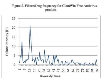
In Fig. 10, the “Fitted FI” graphs are obtained using (6). The expected cumulative failures at each biweekly period are calculated by inserting the scale and shape values from Table II in (2). The corresponding estimated failure for each biweekly period is then obtained from (6). The figure also shows other graphs, which will be explained in the next section when failure forecasting is discussed. These graphs are included in this section to lessen the number of figures.

Figure 10a. Estimated FI for ClamWin Free Antivirus product.

Figure 10b. Estimated FI for MPlayer OS X product.

Figure 10c. Estimated FI for Apache 2 product.

0 200 400 600 800 1000 1200 1400 1600 1800 1 7 ₁₃ _{19 25} _{31 37} _{43 49} ₅₅ ₆₁ ₆₇ ₇₃ ₇₉ ₈₅ ₉₁ ₉₇ 10 3 10 9 11 5 12 1 12 7 13 3 13 9 14 5 15 1 15 7 Biweekly Time Bu g Fr e q u e n cy 0 2 4 6 8 10 12 14 16 18 1 9 17 25 33 41 49 57 65 73 81 89 97 105 113 Failure Intensity (FI) Biweekly Time

Filtered Bug Pattern Fitted FI Fitted 1-Year FI Fitted 2-Year FI 0 5 10 15 20 25 1 9 17 25 33 41 49 57 65 73 81 89 97 Failure Intensity (FI) Biweekly Time

Filtered Bug Pattern Fitted FI Fitted 1-Year FI Fitted 2-Year FI 0 10 20 30 40 50 60 1 13 25 37 49 61 73 85 97 109 121 133 145 157 169 Failure Intensity (FI) Biweekly Time

Filtered Bug Pattern Fitted FI

Fitted 2-Year FI Fitted 4-Year FI

(7)

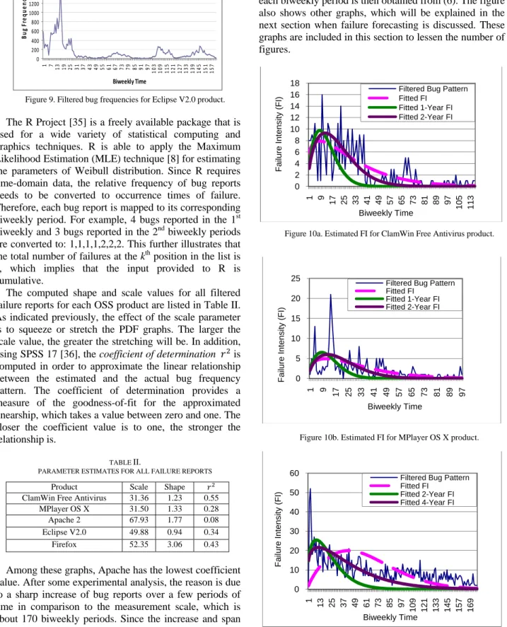
Figure 10d. Estimated FI for Eclipse V2.0 product.

Figure 10e. Estimated FI for Firefox product.

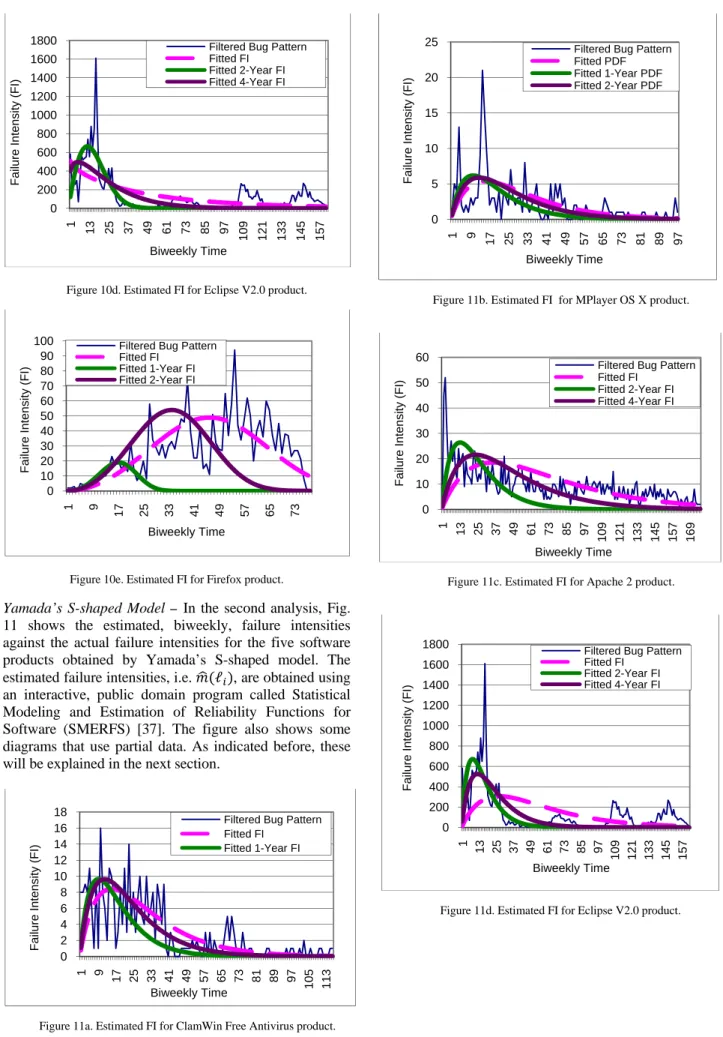
Yamada’s S-shaped Model – In the second analysis, Fig. 11 shows the estimated, biweekly, failure intensities against the actual failure intensities for the five software products obtained by Yamada’s S-shaped model. The estimated failure intensities, i.e. ℓ , are obtained using an interactive, public domain program called Statistical Modeling and Estimation of Reliability Functions for Software (SMERFS) [37]. The figure also shows some diagrams that use partial data. As indicated before, these will be explained in the next section.

Figure 11d. Estimated FI for Eclipse V2.0 product.

0 200 400 600 800 1000 1200 1400 1600 1800 1 13 25 37 49 61 73 85 97 ₁₀₉ ₁₂₁ ₁₃₃ ₁₄₅ ₁₅₇ Failure Intensity (FI) Biweekly Time

Filtered Bug Pattern Fitted FI Fitted 2-Year FI Fitted 4-Year FI 0 10 20 30 40 50 60 70 80 90 100 1 9 ₁₇ ₂₅ ₃₃ ₄₁ ₄₉ ₅₇ ₆₅ ₇₃ Failure Intensity (FI) Biweekly Time

Filtered Bug Pattern Fitted FI Fitted 1-Year FI Fitted 2-Year FI 0 2 4 6 8 10 12 14 16 18 1 9 17 25 33 41 49 57 65 73 81 89 97 105 113 Failure Intensity (FI) Biweekly Time

Filtered Bug Pattern Fitted FI Fitted 1-Year FI 0 5 10 15 20 25 1 9 17 25 33 41 49 57 65 73 81 89 97 Failure Intensity (FI) Biweekly Time

Filtered Bug Pattern Fitted PDF Fitted 1-Year PDF Fitted 2-Year PDF 0 10 20 30 40 50 60 1 13 25 37 49 61 73 85 97 109 121 133 145 157 169 Failure Intensity (FI) Biweekly Time

Filtered Bug Pattern Fitted FI Fitted 2-Year FI Fitted 4-Year FI 0 200 400 600 800 1000 1200 1400 1600 1800 1 13 25 37 49 61 73 85 97 109 121 133 145 157 Failure Intensity (FI) Biweekly Time

(8)

Figure 11e. Estimated FI for Firefox product.

Table III shows the estimated parameters and the coefficient values for the S-shaped model. Similar to the Weibull distribution, the model exhibits a similar pattern of graph estimates among the products.

TABLE III.

ESTIMATED PARAMTERS AND COEFFICEINT VALUES FOR THE OSS

PRODUCTS BASED ON S-SHAPED MODEL

Product

ClamWin Free Antivirus 334 0.07 0.44 MPlayer 214 0.07 0.26 Apache 2 1770 0.03 0.08 Eclipse V.2 22200 0.04 0.07

Firefox 6230 0.02 0.38 Schneidewind’s Model - This model is a concave shaped NHPP, an IEEE standard model for software reliability analysis. The diagrams for the real and estimated failure intensities are presented in Fig. 12. Similar to the S-shaped model, the estimated failure intensities are obtained using SMERFS.

Figure 12d. Estimated FI for Eclipse V2.0 product. Schneidewind’s model could not fit the Firefox failure data. As mentioned previously, one possible reason can be related to the fact that failure data has not stabilized yet and thus the available data is not sufficient for fitting. Table IV lists the estimated parameters and the coefficient values for the other products.

0 10 20 30 40 50 60 70 80 90 100 1 9 17 25 33 41 49 57 65 73 Failure Intensity (FI) Biweekly Time

Filtered Bug Pattern Fitted FI Fitted 1-Year FI Fitted 2-Year FI 0 2 4 6 8 10 12 14 16 18 1 9 17 25 33 41 49 57 65 73 81 89 97 ₁₀₅ ₁₁₃ Failure Intensity (FI) Biweekly Time

Filtered Bug Pattern Fitted FI Fitted 1-Year FI Fitted 2-Year FI 0 5 10 15 20 25 1 9 17 25 33 41 49 57 65 73 81 89 97 Failure Intensity (FI) Biweekly Time

Filtered Bug Pattern Fitted FI Fitted 1-Year FI Fitted 2-Year FI 0 10 20 30 40 50 60 1 13 25 37 49 61 73 85 97 109 121 133 145 157 169 Failure Intensity (FI) Biweekly Time

Filtered Bug Pattern Fitted FI Fitted 2-Year FI Fitted 4-Year FI 0 200 400 600 800 1000 1200 1400 1600 1800 1 ₁₃ ₂₅ ₃₇ ₄₉ ₆₁ ₇₃ ₈₅ ₉₇ 109 121 133 145 157 169 Failure Intensity (FI) Biweekly Time

(9)

TABLE IV.

ESTIMATED PARAMTERS AND COEEFICIENTS VALUES OF THE OSS

PRODUCTS BASED ON SCHNEIDEWID’S MODEL

Product

ClamWin Free Antivirus 10 0.03 0.52

MPlayer 6 0.03 0.24

Apache 2 20 0.01 0.50 Eclipse V.2 360 0.02 0.30

Using Tables II, III, and IV, Table V presents the overall best and worst fits for the five products when the entire failure data is used. Visual comparison of the graphs in Fig. 10-12 supports the results in Table V. For the Apache product, since the beginning failure intervals before reaching a peak is very short and the rest of failure data forms a decreasing exponential graph, Schneidewind’s model, which is an exponential model, was able to obtain a much better fitting compared to Weibull.

TABLE V.

BEST AND WORST FITTING MODELS FOR THE SELECTED OSS

PRODUCTS

Product Best model Worst model ClamWin Free

Antivirus

Weibull Schneidewind MPlayer Weibull Schneidewind Apache 2 Schneidewind S-Shape, Weibull Eclipse V.2 Weibull S-shaped

Firefox Weibull S-shaped

(Schneidewind not able to model)

B. Reliability Prediction

In general, software reliability prediction attempts to forecast the quality of the software system based on the current knowledge such as the failure history. One of the main goals of software reliability prediction is not necessarily determining the future reliability of the product, but rather what needs to be done to achieve a particular level of reliability at a future point of time or whether that level of reliability would be feasible to reach. Since no metric parameter other than the failure history of the selected products is available, the goal of this section is to decide which of the three reliability models predict the future behavior of failures that is closer to the truth based on the partial failure history of the products. Among all reliability models, there is no reliability model to be always superior over the other models. But the failure pattern can be used as a simple way to decide on some models believed to provide a decent prediction. The three models, i.e. Weibull, S-shaped, and Schneidewind are chosen based on this understanding.

Other than the graph estimates for the entire failure data, Fig. 10 also shows the forecasts of failure intensities by Weibull based on partial failure reports. Depending on the interval of collected reports, the prediction length might be different for each product. For example, in Fig. 10a, there are 116 biweekly periods, which is divided into two prediction periods. The first prediction uses the failure data for the first year that is fed into R to arrive at the estimated parameters, i.e. shape and scale. To obtain

the estimated predicted values for the rest of the biweekly periods, the values of these parameters are then used in (6) with the time periods ranging between 1 and 116. Similarly, to predict the future failure for the second prediction period, the failure data for the first two years are used in estimating the parameters. Therefore, the partial failure data for predicting a longer period is lower than that of predicting future failure pattern for a shorter time. For a product like Apache, for which the number of failure reports stretches over a much longer time, i.e. 176 biweekly periods in Fig. 10c, the partial failure data is based on two and four years. So, the first and the second prediction intervals use the partial data for the first two years and the first four years of failure data, respectively. The same approach is used in Fig. 11-12 for the S-shaped and Schneidewind models. From Fig. 10-12, there exists the consistent observation that the prediction accuracy worsens as the prediction intervals are increased. For example, for the ClamWin product, the future failure prediction based on one year of failure data is less accurate in comparison to using two years of failure data. In either case of prediction, i.e. one and two years or two and four years of partial failure data, the remaining interval for predicting the failure pattern is at least one and two years or two and four years, respectively.

One general way to compare the models is to determine which one provides the least difference between the predicted and the actual number of failures. This can be presented in the predicted relative error form (PRE). PRE is the ratio between the difference of failures (observed versus predicted) and the predicted number of failures. Specifically,

.

Table VI shows the PRE values using the cumulative number of failures at the final biweekly period. To produce the observed and predicted values, the early portion of failure data of actual and estimated failures are subtracted from the total number of actual and estimated failures, respectively. The early portion of failures removed from the total number of failures for ClamWin, MPlayer, and Firefox is one year and for Apache and Eclipse is two years. Table VII is similar to Table VI except the early number of failures removed is based on two years (ClamWin, MPlayer, Firefox) and four years (Apache, Eclipse). As the tables show, Schneidewind’s model consistently shows superiority. The next best model is S-shaped.

TABLE VI.

PRE VALUES BASED ON 1(CLAMWIN, MPLAYER, FIREFOX) AND 2 (APACHE, ECLIPSE) YEARS OF FAILURE DATA

Product S-shaped Weibull Schneidewind ClamWin Free Antivirus 2.51 12.54 0.57 MPlayer 1.36 11.12 0.70 Apache 2 10.94 19.29 1.26 Eclipse V.2 56.47 1542.03 7.90

(10)

TABLE VII.

PRE VALUES BASED ON 2(CLAMWIN, MPLAYER, FIREFOX) AND 4 (APACHE, ECLIPSE) YEARS OF FAILURE DATA

Product S-shaped Weibull Schneidewind ClamWin Free Antivirus 2.15 6.96 0.29 MPlayer 1.345 6.49 0.37 Apache 2 4.45 5.53 0.55 Eclipse V.2 364.06 125.59 32.06

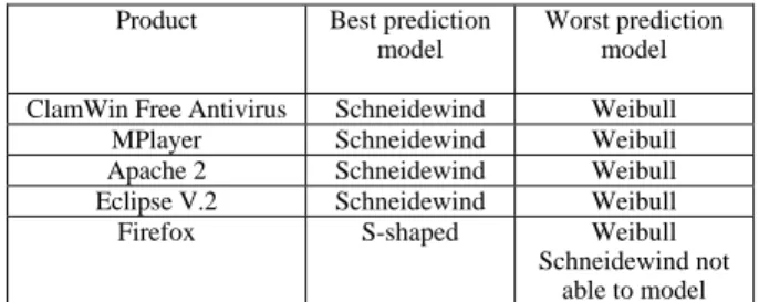
Firefox 0.21 9.03 Not able to model Although the PRE approach is a decent way to realize which model offers a better prediction, it does not capture the trend of prediction over time. PLR is a valuable tool that exhibits the relative trend of prediction of one model versus another, instead of depending on singular values. When comparing two models, as indicated in the Background section, the numerator model is favored over the denominator model if the graph of the PLR values is ascending. Otherwise, the denominator model is favored. Although there might be fluctuations in predictions, the overall trend of the graph will show which model is favored. Fig. 13 presents the PLR graphs for MPlayer when comparing the three models. Between S-shaped and Weibull, the ascending graphs ascertain that the S-shaped model provides better prediction. However, when comparing S-shaped and Schneidewind models, the Schneidewind’s model is favored. This implies that the Schneidewind’s model provides the best prediction. When using PLR for the other products, Schneidewind’s model again exhibits the best accuracy of prediction among the three models. The PLR graphs for the other products are not shown because the trend of graphs is similar and in some instances the denominator values are very small, so that the PLR ratios become undefined. The undefined PLR is the indication that the numerator model is favored.

Figure 13. Comparing failure prediction of Weibull, S-shaped, and Schneidewind models for MPlayer using PLR.

Based on the PLR graphs of all products, Table VIII displays the best and worst prediction models.

IV. CONCLUSION

This study has attempted to compare three prominent reliability models with respect to estimates of failures intensities and failure forecasts against the actual failure data. For the sake of accuracy, rather than depending on a

single failure data source, the bug reports of five popular OSS products are collected and used as input to the three models. The quality of bug analysis heavily depends on comprehensive and accurate recording of bug reports. Also, the lack of a commonly accepted data format for archiving bug reports and efficient algorithms for data filtering have added to the complexity of failure data analysis.

TABLE VIII.

BEST AND WORST PREDICTION MODES FOR THE SELECTED OSS

PRODUCTS

Product Best prediction model

Worst prediction model ClamWin Free Antivirus Schneidewind Weibull MPlayer Schneidewind Weibull Apache 2 Schneidewind Weibull Eclipse V.2 Schneidewind Weibull

Firefox S-shaped Weibull

Schneidewind not able to model The study has further used three metrics for comparison purposes among the models. The determination coefficient is an easy metric for initial understanding of goodness-of-it. The coefficient values are used to compare the accuracy estimates of the three models based on the entire failure data of each selected OSS product. The second metric, i.e. PRE value, is used to determine which model predicts the best, accurate estimation of accumulative failures at the final biweekly report. As the third metric, PLR has been adopted to compare the prediction accuracy of the three selected models over time.

For the selected products, Weibull has shown to be the best model overall for goodness-of-fit among the three models. This can be visually observed when comparing the Fig. 10–12. But Weibull prediction capability fell below that of S-shaped and Schneidewind models. Specifically, Schneidewind’s model provided the best prediction model for future failures followed by the S-shaped model. Therefore, a model that is able to provide a good fit may not be a good predictor of future failures.

Although there are many reliability growth models, no single model is believed to be a feasible choice for all forms of bug-failure patterns. The selected OSS products all show similar patterns when analyzing their failure data, in that a trend of increasing failure, once reached a peak, is followed by a long, continuous decreasing tail. Therefore, the three models chosen shown to be viable candidates for this study5.

The knowledge gained from this research can be expanded in different directions. One avenue of research is to include other potential statistical models such as Bayesian and Lognormal [8]. Furthermore, it is reasonable to believe that some failure intensities can be considered as outliers [38] that may have tangible effect on the estimated values of model parameters. Hence, an

5_{The reader is referred to [9] for further information on deciding a} possible reliability model for a specific failure pattern.

-150 -100 -50 0 50 100 150 200 250 27 35 43 51 59 67 75 83 91 Log (PLR) Biweekly Time

2 Years FI, S-shape/Weibull 1 Year FI, S-shape/Weibull 2 Years FI, S-shape/Schneidewind 1 Year FI, S-shape/Schneidewind

(11)

interesting research direction is to analyze the impact of outliers on goodness-of-fit and prediction of failures. Finally it is worth to investigate the recalibration of some reliability models, as some studies have shown that model recalibration can be an effective approach to better accuracy of prediction [39].

ACKNOWLEDGMENT

This research is funded in part by Department of Defense (DoD)/Air Force Office of Scientific Research (AFOSR), NSF Award Number FA9550-07-1-0499, under the title “High Assurance Software”.

REFERENES

[1] E.S. Raymond, “The cathedral and the bazaar: musings on linux and open source by an accidental revolutionary”, 2nd Ed., O’Reilly, 2001.

[2] SourceForge, http://sourceforge.net.. [3] Bugzilla, http://www.bugzilla.org.

[4] A. Mockus, T.R. Fielding, and J.D. Herbsleb, “Two case studies of open source software development: Apache and Mozilla”, ACM Transactions on Software Engineering and Methodology, vol. 11, no. 3, July 2002, pp. 309-346. [5] Y. Zhou and J. Davis, “Open source software reliability

model: an empirical approach”, The 5th Workshop on Open Source Software Engineering, May 2005, pp. 1-6.

[6] T.R. Moss, The Reliability Data Handbook, ASME 2005. [7] S. Yamada, M. Ohba, and S. Osaki, “S-shaped reliability

growth modeling for software error detection”, IEEE Transactions on Reliability, vol. R-32, 1983, pp. 475-478. [8] H. Pham, “System Software Reliability”, Springer, 2006. [9] P. Lakey, A. Neufelder, “System and Software Reliability

Assurance Notebook”, Rome Laboratory, 1997.

[10]N.F. Schneidewind, "Analysis of Error Processes in Computer Software”, Sigplan Note, vol. 10, no. 6, 1975, pp. 337-346.

[11]IEEE Reliability Society, “IEEE recommended practice on software reliability”, IEEE Std 1633-2008, June 2008. [12]American Institute of Aeronautics and Astronautics,

Recommended Practice for Software Reliability, ANSI/AIAA R-013-1992, Feb 1993.

[13]M.R. Lyu, Handbook of Software ReliabilityEengineering, McGraw Hills, 1996.

[14]N.F. Schneidewind, T.W. Keller, "Application of Reliability Models to the Space Shuttle," IEEE Software, July 1992, pp. 28-33.

[15]J.D. Musa and K. Okumoto, “A logarithmic poisson execution time model for software reliability measurement”, 7th Int’l Conference on Software Engineering(ICSE), 1984, pp. 230-238.

[16]J.De.S. Coutinho, “Software reliability growth”. IEEE Symp. Computer Software Reliability, 1973, pp. 58-64. [17]Z. Jelinski and P.B. Moranda,”Software reliability

research”, in Statistical Computer Performance Evaluation, W. Freiberger, Ed., Academic Press, 1972, pp. 465-484. [18]M.L. Shooman, “Probabilistic models for software

reliability prediction”, in Statistical Computer Performance Evaluation, W. Freidberger, Ed., New York: Academic Press, 1972, pp. 485-502.

[19]McCabe, T.J, “A Complexity Measure”, IEEE Trans Soft Engineering, vol. SE-2, no. 4, 1976.

[20]M.H. Halstead, “Elements of Software Science”, Elsevier, New York, 1977.

[21]A.L. Goel and K. Okumoto, “A time-dependent error-detection rate model for software reliability and other

performance measure”, IEEE Transactions on Reliability, vol. R-28, 1979, pp. 206-211.

[22]M. Ohba, “Software reliability analysis models”, IBM. J. Research Development, vol. 21, no. 4, 1984.

[23]H. Pham, L. Nordmann, “A generalized NHPP software reliability model”, 3rd Int’l Conference on Reliability and Quality in Design, 1997.

[24]K.S. Trivedi, Probability and Statistics with Reliability, Queuing and Computer Science Applications, 2nd Ed., John Wiley, 2002.

[25]B. Littlewood and J.L. Verrall, “A bayesian reliability model with a stochastically monotone failure rate”, IEEE Trans on Reliability, vol. R-23, June 1974, pp. 108-114. [26]H.S. Kan, Metrics and Models in Software Quality

Engineering, 2nd Ed., Addison-Wesley, 2003.

[27]I. Koren and C.M. Krishna, Fault-Tolerant Systems, Morgan Kaufmann, 2007.

[28]R.C. Cheung, “A user-oriented software reliability model”, IEEE Trans Software Eng., vol. 6, no. 2,1980, pp. 118-125. [29]S.S. Gokhale, M.R. Lyu, and K.S. Trivedi, “Reliability

simulation of component-based software systems”, Proceedings of 9th Int’l Symposium on Software Reliability Engineering, 1998.

[30]W.L. Wang, Y. Wu and M.H. Chen, “An architecture-based software reliability model”, Proceedings of Pacific Rim Int’l Symposium on Dependable Computing, 1999. [31]S. Yacoub, B. Cukic and H.H. Ammar, “A software-based

reliability analysis approach for component-based software”, IEEE Trans on Reliability, vol. 53, no. 4, 2004. [32]B. Littlewood and J.L. Verrall, “A bayesian reliability

growth model for computer software”, Applied Statistics, vol. 22, 1973, pp. 332-346.

[33]A.P. Dawid, "Present position and potential developments: Some personal views: Statistical theory: The prequential approach",Journal of the Royal Statistical Society, vol. 147, no. 2, 1984, pp. 278-292.

[34]B. Littlewood, A. Ghaly, P.Y. Chan, “Tools for the Analysis of the Accuracy of Software Reliability Predictions”, in Soft. Sys. Design Methods, J.K. Skwirznski, Ed., NATO ASI Series, vol. F22, 1986, pp. 299-335.

[35]R Project, http://www.r-project.org/. [36]SPSS, http://www.spss.com/statistics. [37]SMERFS, http://www.slingcode.com/smerfs/.

[38]W.J. Conover, Practical Nonparametric Statistics, 3rd Ed., John Wiley, 1999.

[39]S. Brocklehurst, B. Littlewood, “New ways to get accurate reliability measures”, IEEE Soft., 1992, pp. 34-42.

Cobra Rahmani received her MS degree in Software Engineering from Iran University of Science and Technology. She is a PhD student in Information Technology at University of Nebraska-Omaha, USA. Her research interests are Software Architecture, Reliability, and Requirement Formalization. Azad Azadmanesh received the PhD degree in Computer Science from University of Nebraska-Lincoln, USA. He is a professor at University of Nebraska-Omaha. His research interests include Network Survivability, Fault-Tolerance, Reliability Modeling, and Distributed Agreement.

Lotfi Najjar holds a PhD in Industrial Engineering with minor in MIS from University of Nebraska-Lincoln. He is currently with the Information Systems and Quantitative Analysis Department at University of Nebraska-Omaha. His research interests are in the areas of Quality Information Systems, Software Quality, Systems Reliability, BPR, and Data Mining.