Brownian motion: a random walk approximation

(1)

Title:

Author:

Advisor:

Department:

Academic year:

Degree in Mathematics

Sergio Gutiérrez Moya Oriol Serra Albó Mathematics

2017-2018

(2)

Universitat Politècnica de Catalunya

Facultat de Matemàtiques i Estadística

Degree in Mathematics

Bachelor’s Degree Thesis

Brownian motion: a random walk

approximation

Sergio Gutiérrez Moya

Supervised by Oriol Serra Albó

June, 2018

(3)

(4)

Thanks to my family and friends, who have supported me along this amazing venture. I wish to express my sincere thanks and indebtedness to Dr. Oriol Serra for supervising and leading me throughout this work. I also place on record my gratitude to all Faculty professors for providing me with valuable guidance and encouragement.

(5)

(6)

Abstract

Brownian motion is one of the most used stochastic models in applications to financial mathematics, communications, engineeering, physics and other areas. Many of the central results in the theory are obtained directly from its definition as a continuous process. As a mathematical object, Brownian motion also have some special and important properties that make it fundamental to understand related mathematical fields and state-of-the-art concepts.

The purpose of this work is to review a relatively recent approach which allows to reobtain these results via a random walks approximation. Brownian motion is the stochastic limit of suitably nested random walks, but some technical details are need to be checked in order to guarantee the conver-gence. The applications of this particular approach include the local time of Brownian motion and the Black-Scholes model in financial mathematics.

Keywords

Brownian motion, Wiener process, Random Walk, local time, Black-Scholes model, stochastic pro-cess, Markov chain, probability theory.

(7)

1. Introduction

Universe is sorrounded by a wide range of phenomena to which mathematical models provide a valu-able tool of analysis and description. A mathematical model, in order to be useful, must satisfy two basic principles: accuracyandsimplicity. It is clear that any model should be precise when describing a certain event, otherwise conclusions coming from it would be worthless. Simplicity is more subtile. Recalling Occam’s razor principle, models should not make unnecessary assumptions. Provided a model is accurate, it comes useful to choose the less sophisticated, so that analyzing it in depth results into an easier procedure.

This work is devoted to the study of Brownian motion, the most globally spread stochastic model in the study of random phenomena. Its strength comes from the two features mentioned above, which Brownian motion widely satisfies. The simplicity of the Brownian motion arises from its back-ground discrete model of random walks, based on simple random independent binary inputs. On the other hand, Brownian motion is based on the normal distribution, which through the Central Limit Theorem, enjoys a universal character describing the addition of a large number of independent random inputs.

This establishes the main motivation of this work. What is the essence that makes Brownian motion so special? Which are the components in its core that transform it into ’the model’ for ran-domness? These questions will serve us as a starting point with the objective of cracking Brownian motion. After that, we will have a better understanding of the general ideas hidden behind it, which are fundamental to use in those models which are of our interest. However, Brownian motion itself would not be that relevant if it were not for its numerous applications in many fields. We also include a discussion on some of these applications.

From a global scale, this work intends to give a general view of Brownian motion. Firstly, a solid background is set: definitions, properties and results about regularity and its ordered random struc-ture. Next, a construction of the Brownian motion through random walks will be given. Brownian motion is often described as a stochastic limit of random walks. Actually, it is so, but it is not that simple. Just a sequence of random walks is not enough to obtain a Brownian motion, but a suitably nested sequence of random walks that inherit its correlation along the sequence has to be defined in a delicate construction. This is a hard task that is completely detailed in this work. With little details left, an exhaustive proof of the convergence to Brownian motion is given. Our milestone is to produce a mathematically robust work, hence it is essential to add all details of the construction. We come up with the desired conclusion, which is the result used in the forthcoming applications.

The relevance of Brownian motion becomes aparent when looking at any text on random pro-cesses. Probably, when it was firstly introduced by the botanist Robert Brown in 1824, nobody was conscious about the impact it was going to have on the coming decades and centuries as a model in Statistical Physics, Mathematical Finances, Electrical Engineering and as a central object in Prob-ability Theory, Statistics, Geometry among many other areas in mathematics and applications. It was one of the topics treated by Albert Einstein which eventually laid empirical foundations of the corpuscular nature of matter in Theoretical Physics, and as ealrly as 1900 it was already considered by Louis Bachelier as a model for the stock market evolution. Both directions have given substantial developments up to our days.

(9)

1 Introduction

This work is organized as follows. We begin by giving a short general description and classifi-cation of stochastic processes, so that we can see fundamental properties of Brownian motion that also apply to other stochastic processes. This is the object of chapter 2. Following this chapter, special emphasis is given to Markov chains for two reasons: the particular vocabulary that appears recurrently throughout this thesis with which we need to be familiar with, and the crucial fact that Brownian motion and random walks are Markov processes, thus we need a good understanding of them.

After this introductory material, we are ready to thrive to the most classical view of Brownian motion: the probability approach. In chapter 4 the abstract probabilistic definition of Brownian motion is presented and some basic properties are proved. The existence of Brownian motion from its formal definition is backed up by the Wiener’s theorem. The proof of this theorem uses an im-portant technique which appears recurrently in this work. Surprisingly, some other imim-portant results are straightforward, such as the scaling invariance and the non-differentiability. As a Markov chain, Brownian motion has some special properties that makes it even more particular. They are studied in chapter 5. The most breathtaking is the reflection principle, not only by its own interest, but also because of its direct consequences.

Since its introduction at the beginning of the19th century, the feature which has given Brownian motion a greater entity is its several applications in science. From pure mathematics to natural sciences, Brownian motion has been a key piece in research throughout the time, allowing ground-breaking advances that make science progress. In this thesis two applications will be visited: Brownian local time and the Black-Scholes model.

We aim at replicating these results not only through a classical approach, but also using embed-ded random walks. To do so, thetwist and shrinkconstruction of Tamas Tsabados will be followed. Actually, chapter 6 is devoted to check that there is convergence to Brownian motion of random walks defined in this particular way. It contains the core of this work, the way Brownian motion can be approached through nested random walks. More precisely, some accurate bounds will be given as illustration. These inequalties will be instrumental to discuss later approximations of this approach. Many technical details are necessary to give an accurate proof. The lemmas stated lead to the a final theorem that asserts the desired convergence.

As an almost surely, nondifferentiable stochastic process, Brownian motion produces very irregu-lar paths, in the sense that changes of value happen suddenly as the result of a random law. Thus, it could be of interest to analyze the time distribution that the process spends at a given level, from a probability point of view. This gives rise to Brownian local time. We approximate it via the classical results, the Trotter’s theorem, and also by using the twist and shrink construction. The later is followed from the article [10], but some details are ommited due to its technical complexity and extension. The classical proof is based on the idea that underpins the proof of the Ray-Knight

(10)

1 Introduction

Lastly, chapter 8 turns around the Black-Scholes model. It was a significant breakthrough in financial mathematics, as finally there was a unique formula to price some financial claims, and even for some of them, explicit formulas exist. First, a brief introduction on changes of measure is given, for reasons concerning risk-neutral pricing, in which much of financial options theory is based. Also, we state the fundamentals of the model in order to set a framework of reference. The approach used to retrieve the results is based on [11]. It is relatively straight to find these formulas using simple probability arguments and thetwist and shrink embedding of random walks.

This work is based on the recent monography by Peters Morter and Yuval Peres entitledBrownian motion[8] and on a series of papers by Tamás Szabados and his collaborators [9,10,11], which were on the background motivation of this work. On one side, a thorough understanding of Brownian motion in the probabilsitic framework, and on the other side the detailed description of Brownian motion from the perspective of Random Walks for a better understanding of its nature and some of its applications.

(11)

2. Overview of Stochastic Processes

Consider a probability space (Ω,A,P), and a random variable X :Ω−→ R. Ω, the set of possible successes, which a probability of occurrence is determined on R and A is a σ-algebra. Stochastic processes are the most general extension on A of random variables. Instead of a random distribu-tion for the variable, an addidistribu-tional index set I is introduced, so that the distribution evolves over time. Another level of difficulty are random vectors. Now, events are not identified by numbers but a vector. Probability distributions (joint, marginals, conditionals) play a more important role when we try to describe randomness. Stochastic processes appear to give a infiniteness version of vectors extended to the whole real line, or a subset of it I depending on the case. They can be seen from two different perspectives, as they have two arguments: the state-space elements ω ∈Ω

and a temporal parameter t. Hence two rather different interpretations can be done: fixt0, observe

how the state-space in configured at that time, or fixed ω ∈Ω, a path is generatedpath along the time. The latter interpretation will be of essential importance for us in some sections, as we will be interested in the analysis of continuity and differentiation of Brownian paths. But, it is possible to find a connection of this two visions of a stochastic process in some cases, which is given by

Ergodic theorems. They are a series of theorems, with applications in many mathematicals branches, in particular in probability theory that allow us to study the assymptotic properties of some random processes, such as Makov chains.

Also, it will be fundamental to decide or argue if a given process actually can exist and is well-defined. In the case of Brownian motiontwo different approaches will be detailed in this work. One of them is underpinned by the so-called Wiener’s theorem, which definitely states that Brownian motion exists. The proof of this theorem was vital for the historical development of theory and applications that followed.

A first clear classification of processes is determined by the index parameter T. IfT = (0,1...)

then the process Xt is said to be adiscrete-timestochastic process. IfT = [0,∞), thenXt is called

a continuous timestochastic process.

Some general properties identify important classes of random processes. They not only describe natural features of random processes, but also allow mathemtical analysis in greater depth. These are the different stochastic processes:

a) Processes with stationary independent increments

If the random variables

Xt2 −Xt1,Xt3 −Xt2, ... ,Xtn−Xtn−1

are independent for all t1<t2 <· · ·<tnthenXt is a process with independent increments (also

allowing a first time t0). Even if restrictive, this condition is satisfied by a wide class of random

processes. It allows to obtain all joint distributions from the knowledge of the one for Xt and

every t.

If the distribution of incrementsX(t+h)−X(t)depends only on the length ofh and not on the time t, then process is said to havestationary increments.

(12)

2 Overview of Stochastic Processes

b) Markov Processes

These processes generalize the idea of Markov chains (see Section 3) for a wider range of state-space. The idea of these processes is that what happens in the future is only determined by the present of not the past, that cannot alter the future whatsoever, given the present. This leads to the Markov propertyof the process. In fact, conditional to an initial distribution of the state-space, the process is uniquely determined by a transition probability matrixbetween states that provides how states evolve in the Markov process. More formally, for eacht1 <t2 <...tk

Pr(Xt =x|Xt1 =x2,Xt2 =x2...Xtk =xk) =Pr(Xt=x|Xtk =xk)

The two main stochastic process that are considered in this work, random walks and Brownian motion are Markov processes.

c) Martingales

The idea of martigales is similar to the one of Markov processes but in this case, instead of a probability idistribution and a transition matrix, the expectation of the process is the defining property for martingales. In other words, let {Xt}a real-valued stochastic process. We say that

{Xt}is a martingale if E(|Xt|)<∞ for all t, and for anyt1 <t2 <· · ·<tk <tk+1

E(Xtk+1|Xt1 =x1,Xt2 =x2, ...Xtk =xk) =xk

This model is used in gambling games where fair games need to be defined, and after a game the player expects to have the same amount of money of the beggining of the game. They are also used in finance for events forecasting. Again, this property holds for Brownian motion and random walks.

d) Stationary processes

The concept of stationarity has very widely meanings, but in stochastic processes’ context, we say that a process Xt is stricly stationaryif the joint distributions

(Xt1+h, ...Xtn+h) and(Xt1, ...Xtn)

are equal for all h > 0 and for any choice of t1, ... ,tn. A stochastic process Xt is said to be

widely sense stationary if the process has finite second order moments and if Cov(Xt,Xt+h) =

E(XtXt+h)−E(Xt)E(Xt+h) depends only on h for all t. A stationary process is stationary in

wide sense, but the converse is not necessary so, it is a wider assumption (only at expectation level).

In addition to this processes, there are also renewal processes and point processes. They do concern the contents of this work, therefore no details about them are given. In interested, more information can be found in [6]. These are the main types of stochastic processes. As radom walks and Brownian motion are included in some types of the processes described, it is easier to extract information about them, or conversely, some properties of them can be generalised.

(13)

3. Markov chains

Markov chains are probably, together with Brownian motion, one of the most broadly studied stochas-tic processes. In this section, some of its most outstanding properties will be studied: from recurrent or transient states of discrete-time Markov chains to the connection of random walks to them through an assymptotic approxiamtion.

Despite this wide range of basic properties, the defining property that all Markov chains share is known asMarkov property. Getting straight to it, it can be interpreted as a past independence given the present, in other words, for chains only matters the very last step. More formally, consider a sequence of random variables X0,X1, ...Xn, the property states that:

Pr(Xn+1 =xn+1|Xn=xn,Xn−1=xn−1...X0 =x0) =Pr(Xn+1=xn+1|Xn=xn)

Markov chains and Markov processes are used in several applications, such as, weather forecast, simulation, game theory, birth-death processes (Galton-Watson )..., and, more importantly for us, in finance, in order to examine possible situations in which an arbitrage operation can be executed or to determine the volatitlity of prices of an underlying asset.

Although it is not proved in this chapter, Brownian motion is a continuous-time Markov chain, which in fact is also a martingale. Thus, in order to approximate it, we need a discrete process that taken to the limit converges to a Brownian motion. Here random walks appear to be exactly what fills the gap. It will be the tool used to approach Brownian motion through a discrete process. This joining process is detailed in chapter 6, where it will be seen that the embedding should be done suitably, so that we get a convergent process.

Markov chains are the vast majority of Markov processes. However, apart from Markov chains, there exist other Markov processes, which have more general state spaces, such as nonnumerable, which are not possible for Markov chains. TheMarkov propertystill holds for them. In this work, we will only work with discrete time Markov chains, as they will be our interest to see some properties of Brownian motion and random walks. Another type of Markov chains are continuous-time Markov chains. They have very similar properties to the discrete time chains, with some modifications. However, the general theory would be too extense to develop in deepth, and we will focus on the Markov property of Brownian motion in chapter 5, where important consequences will be deduced.

3.1 Discrete-time Markov Chains

Let I be a countable set. We calli ∈I the set of all possible states of the Markov chain. Then,I is known as the state-space. Consider a probability space(Ω,A,P) and adistribution of probabilityλ

in this space. For a random variableX :Ω→I, set:

λi =P(X =i) =P(ω:X(ω) =i)

Definition 3.1. We say that a matrixP = (pij,i,j ∈ I) is stochastic if every row (pij,j ∈ I) is a

probability distribution.

This condition on matrices representing the states transition is natural, as for a given state, a probability distribution will be established among all states, including itself. In this case, the transition to the next step is well-defined.

(14)

3 Markov chains

Definition 3.2. We say that (Xn)n≥0 taking values in I is a Markov chain with initial distribution λ= (λi)i∈I and trasition matrixP if

(1) X0 has a distributionλ;

(2) for n ≥ 0, conditional on Xn = i, Xn+1 has a distribution (Pij :j ∈ I) and is independent of

X0,X1, ... ,Xn−1.

If the previous conditions are satisfied, for simplicity, we say that(Xn)n≥0isMarkov(λ,P). Moreover,

it is time-homogeneous, since P does not change with time. From the definition of Markov chains

it is clear that:

Theorem 3.3. A discrete-time random process (Xn)0≤n≤N isMarkov(λ,P)if and only if

∀i0,i1, ...iN ∈I P(X0=i,X1 =i1, ... ,XN =iN) =λi0pi0i1pi1i2· · ·piN−1iN (3.1)

A first-stage result on Markov chains is theweak Markov property. It is weak because later we will see a generalisation of it.

Theorem 3.4. (Weak Markov property). Let (Xn)n≥0 be Markov(λ,P). Then, conditional on

Xm =i,(Xm+n)n≥0 is Markov(δi,P) and it is independent of the random variablesX0,X1, ... ,Xm.

A Markov chain can be very difficult to understand globally, but sometimes it is possible to split it in differents parts, so that its structure becomes easier to interpret and analize.

Definition 3.5. We say thati leads to j (and write i →j) if

Pi(Xn=j for somen ≥0) :=Pi(Xn=j for somen≥0|X0=i)>0

Ifi →j andj →i, then we say thati communicatesj (write i ↔j).

From definition and some basic properties, it is easy to check that ↔ satisfies the conditions of an equivalence relation, whence it partitionsI intocommunicating classes. We say thatC is aclosed classif

i ∈C i →j, implyj ∈C

In other words, a closed class is a class from where it is not possible to scape. Particularly, if {i}is a closed class, the state is said to be absorbing. A chain that has one unique communicating class is called irreducible.

3.2 Hitting times, recurrence and transience

Consider a Markov chain (Xn)n≥0, with state-spaceI and a subset A⊂I.

Definition 3.6. Thehitting timeof a random variable: HA(ω) :Ω→ {0,1, ...} ∪ {∞}is defined as:

HA(ω) =inf{n≥0 :Xn(ω)∈A}

The probability of hitting A starting fromi is:

hA_i =_Pi(HA<∞)

(15)

3 Markov chains

Definition 3.7. A random variable T :Ω→ {0,1, ...} ∪ {∞} is called astopping time if the event

{T =n} denpends only on X0,X1, ... ,Xn.

The most plausible interpretation of this definition is that just by observing the past of the process, it is known when a certain event is going to happen. There are many types of random variables that involve stopping times, but the following will be object of study in this project.

Example 3.8. Thefirst passage timerandom variable:

Tj =inf{n≥1 :Xn=j}

is a stopping time. only has to be checked that:

{Tj =n}={X16=j, ... ,Xn−1 6=j,Xn=j}

Now, we provide a stroger form of Theorem 3.4, using stopping times and its properties.

Theorem 3.9. (Strong Markov property)Let(Xn)n≥0 be aMarkov(λ,P)and let beT a stopping time of (Xn)n≥0. Then conditional on T < ∞ and XT = i, (XT+n)n≥0 is Markov(δi,P) and

independent of X0,X1, ...XT.

Actually, we are more interested in a generalisation of Example 3.8, considering the r-th passage time T_i(r) to statei

T_i(0)(ω) = 0, T_i(r+1)(ω) =inf{n ≥T_i(r)(ω) + 1 :Xn=i}.

Definition 3.10. The length of the r-th excursion to i is:

S_i(r)= (

T_i(r)−T_i(r−1) ifT_i(r−1)<∞

0 otherwise

We denote the number of visits Vi to i by:

Vi = ∞ X n=0 1_{_X_n₌_i_} Then, Ei(Vi) :=E(Vi|X0 =i) =Ei _X∞ n=0 1{Xn=i} = ∞ X n=0 Ei(1{Xn=i}) = ∞ X n=0 Pi(Xn=i) = ∞ X n=0 p(_iin),

where the index i denotes the initial statei, and therefore, we are describing the probability (or the mean) of returning to the state i ∈I, respectively.

We compute the distribution of Vi under Pi in terms of the return probability:

(16)

3 Markov chains

Lemma 3.11. Forr = 0,1..., we haveP(Vi >r) =fir

Proof. We prove the result by induction over r. Forr = 0 it is clearly true. For r ≥1 it hold the

{Vi >r}={Ti(r)<∞}. If it is true forr, then:

Pi(Vi >r+ 1) =Pi(Ti(r+1) <∞) =Pi(Ti(r)<∞ andS

(r+1)

i <∞)

=_P_i(S_i(r+1)<∞|T_i(r)<∞)_P_i(T_i(r)<∞) =fifir =fir+1

Definition 3.12. We say that a statei is recurrentif:

Pi(Xn=i for infinitely many n) = 1

Alternatively, we say that a state istransientif:

Pi(Xn=i for infinitely many n) = 0

Theorem 3.13. The following dichotomy holds:

(1) IfPi(Ti <∞) = 1, then i is recurrent and P∞i=0p (n)

ii =∞

(2) IfPi(Ti <∞)<1, then i is transient andP∞i=0p (n)

ii <∞

Proof. IfPi(Ti <∞) = 1, then by Lemma 3.11,

Pi(Vi =∞) = lim_r_→∞Pi(Vi >r) = 1.

Thus, i is recurrent and

∞ X n=0 p_ii(n) =Ei(Vi) =∞. Conversely, if fi =Pi(Ti <∞)<1, ∞ X n=0 p_ii(n) =_E_i(Vi) = ∞ X r=0 Pi(Vi >r) = ∞ X r=0 f_ir = 1 1−fi <∞.

But for more generalisation in terms of the state-space, the preceding dichotomy can be extended to a class property. In other words:

Lemma 3.14. LetC be a communicating class. Then either all states inC are recurrent or transient. Proof. Take any pair of statesi,j such thati is transient. Then, there existm,n≥0such thatp(_ijn)

and p_ji(m), then, for allr≥0,

p_ii(n+r+m)≥p_ij(n)p_jj(r)p(_jim). Thus, if i is transient, ∞ X r=0 p_jj(n)≤ 1 p_ij(n)p_ji(m) ∞ X r=0 p(_iin+r+m)<∞.

(17)

3 Markov chains

3.3 Random Walks

Random walks are one type of Markov chains that require especial attention in this work due to their close connection to Brownian motion. They are also used in many applications in science and tech-nology, embracing the model of a particle moving in a gas or to study the dynamic of a population, entre others. The first example for instance, is surprising as the reader could think of the movement of a particle as a continuous motion. Actually, it is, but in models and simulations continuous data and time intervals are impossible to get and there random walks appear as a good approximation to brownian motion. In principle, the motion could be modelled using other ideas and approximations, but as we will see later, brownian motion can be retrieved from a random walk taken to the limit of the discretization of Zn grid with an appropiate scale.

A particular reason why they shoud be carefully studied is because random walks have a non-finite state space, what means that though its is irreducible and closed, it may be nonrecurrent. However, combinatorail arguments will be given to solve the problem of recurrence of random walks in low dimensions.

Remark 3.15. (Stirling’s formula) For n sufficiently large, n! ≈ √2πn(n_e)n, where ≈ denotes an assymptotic equivalence of both expressions.

For example, if a one-dimensional random walk is considered, the probability of return after an odd number of steps is zero. For even number of steps, the probability of return is:

p₀₀(2n)= 2n n ! pnqn≈ (4pq) n √ nπ .

In the symetric case, p=q= 1₂,pq= 1₄ and thus, for someN and all n≥N:

p₀₀(2n)≥ 1 2√2πn ≈ 1 √ nπ. In consequence, we have: ∞ X n=N p(2₀₀n)≥ √1 π ∞ X n=N 1 √ n =∞

So the symetric one-dimensional random walk is recurrent. In the non-symetric case, 4pq =r <1, and for someN: _∞

X n=N p(2₀₀n) ≤ √1 2π ∞ X n=N rn<∞,

what shows that the one-dimensional random walk is transient, and by symmetry it also holds for

P∞

n=Np

(2n)

ii for any state i. In dimension two, this property still holds, due to the fact that the

harmonic series is divergent, but from dimension three on, the series analysed are convergent and hence, the random walk comes back to the origin infinitely many times with zero probability. In oder to connect random walks with discrte time Markov chains it is useful to introduce the so-called

Chapman-Kolmogorov equations. These equations describe the relation between states in a Markov chain via the transition probabilities that uniquely determine the chain, up to an initial distribution.

Chapman-Kolmogorov equations are:

pij =

X

k∈I

pikpkj

These equations are not of interest in this work, but for example, they are useful to derive the partial differential equation that a Brownian satisfies.

(18)

4. Introduction to Brownian motion

Brownian motion has its origins in the19th. century, when the british scientist R. Brown discovered it by studying the erratic movement of particles on the surface of a liquid. The way he described the motion of particles was named after R. Brown, and was called Brownian motion. However, the concept today has been devolvoped and many generalizations and variations have been introduced. Actually, Brownian motion is widely used in many fields, and its construction and definition gives it some particular properties that make it appropiate for some applications. Usually it appears when in the process handled some uncertainty takes place. Its utility comes from the fact that it has no bias and, therefore, it faithfully simulates nature phenomena that happen in real life.

Suppose the motion of a particle is to be analysed. On the macroscopic level it is not clear at all which will be the path described by the particle at all. But, some inferences can be done when microscopic level is studied. At this level, we see that at any step of it, the particle undergoes a dis-cretepath which is modeled by a random walk. Say Snis the random walk started atX0. Every step

is a random variable that takes the valueXk =±1with equal probability, and thenSn=S0+Pni=1Xi.

However, some results are surprising, because not all features of the microscopic view will have an effect on the macroscopic view. In other words, it is possible to obtain similar path for random walks that share mean and covariance matrices. That makes Brownian motion a very general object, which will link different processes.

Physical interpretation aside, the objective of this section will be making a first approach to its most famous construction and visiting basic properties that will be the seed for the following devel-opments, where more specific topics will be discussed. This will be a fist overlook of the macroscopic figure generated by the process.

4.1 A joint probabilities approach. The Wiener process

Brownian motion is usually defined by a process that must satisfy some conditions. This definition is very versatile, as it allows to study it using arguments underpinned by the normal distribution. Since this distribution is well-known, it requires a softer introduction to acquire a first idea of the nature of this particular process. However, it must be ensured that the definition gives raise to the process desired. This is given by the Wiener’s theorem. After this is done, the random walk approach is more sensitive, provided the local behaviour of the process.

Definition 4.1. A stochastic process{X(t) :t ≥0} is a Brownian motionif:

i) Paths are almost surely continuous for all t≥0.

ii) Every increment X(t+s)−X(s) is normally distributed with mean0 and variancet.

iii) for any t1 <t2 <t3 <t4, the increments: X(t2)−X(t1) andX(t4)−X(t3) are independent

with the distributions specified in ii).

(19)

4 Introduction to Brownian motion

This definition has many important consequences that are followed almost inmediately from it. The first remarkable fact is that Brownian motion satisfies the Markov property, as the distribution of the increments only depends on the time elapsed independently of the values taken by the random variable. More formally,

Pr(X(t)≤x|X(tk)≤xk, ...X(t0)≤x0) =Pr(X(t)≤x|X(tk)≤xk).

It is particularly interesting to compute easily the previous probability and the joint probability of the increments from the definition of Brownian motion.

p(x−x0,t−t0) :=Pr(X(t)≤x|X(t0)≤x0) =Pr(X(t)−X(0)≤x−x0) = _p 1 2π(t−t0) Z x−x0 −∞ e− y2 2(t−t₀₎_dy

Now recall that, from a very basic convolution product, the sum of normal random variables is also normal, so the last part of the definition as, for anyt1 <t2 <t3:

X(t3)−X(t1) = (X(t3)−X(t2)) + (X(t2)−X(t1))

Applying recurrently the Markov property and the independence assumed by hypothesis, using the same notation it holds that the joint probability distribution of increments in terms of the normal density function is:

f(x1, ...xn) =p(x1,t1)p(x2−x1,t2−t1)· · ·p(xn−xn−1,tn−tn−1)

4.2 Wiener’s theorem

The next step is to show that a process defined as above exists, that is, the conditions given are compatible and define a unique process. Previously it is convinient to proof this result:

Lemma 4.2. LetX ≥0 be a non-negative random variable andp>0, then:

E(Xp) =

Z ∞

0

pxp−1P(X >x)dx

Proof. This is a generalization of the result already known for p = 1 and the proof is mainly the same, with some modifications using the Fubini’s theorem.

E(Xp) = Z ∞ 0 xpf(x)dx = Z ∞ 0 Z x 0 ptp−1f(x)dtdx = Z ∞ 0 Z ∞ t ptp−1f(x)dxdt = Z ∞ 0 ptp−1P(X >t)dt

Reviewing again the definiton of the process, it seems that the conditions imposed to marginals densities of the process can lead to a contradiction or may generate discontinuous paths. This is the main concern of the following theorem. In order to prove it, we will construct Brownian motion as a uniform limit of continuous functions, producing a continuous limit process. Mainly, dyadic intervals will be used to generate the distributions imposed, and then this properties will be extended to any interval.

(20)

Theorem 4.3. (Wiener’s theorem)Brownian motion exists.

Proof. Consider the set of D = ∪DN, with DN defined as the set of integer multiples of 2−N in

[0,∞)forN = 0,1,2, .... The steps to follow to complete this proof are delicate, from point of view of mathematical analysis. First we will construct a Brownian motion for some set of indeces and then the difficult task will be how to extend it to the semi-real line continuously and see that, the extension is a Brownian motion.

For any t ∈D, consider an independent Gaussian random variable Yt with mean0 and varaince 1.

For t ∈D0=Z+ set: Bt = t X i=0 Yi

then,Bt is a Brownian motion indexed byD0. Now, by induction we should see that this process can

be extended for all other indexesDN as a Brownian motion. Suppose that(Bt :t∈D0)is brownian

motion for DN−1. Fort ∈DN\DN−1 set r =t−2−N ands =t+ 2−N ⇒r,s ∈DN−1

Consider Zt = 2− N+1 2 Y_t Bt = 1 2(Br +Bs) +Zt

The new increments obtained are:

Bt−Bs = 1 2(Bs−Br) +Zt Bt−Bs = 1 2(Bs−Br)−Zt

Then with a little compututation we get:

E[(Bt−Br)2] =E[(Bs−Bt)2] = 1 42 −(N−1)_{+ 2}−(N+1) _{= 2}−N E[(Bt−Br)(Bs−Bt)] = 1 42 −(N−1)₋₂−(N+1) _{= 0}

Thus, the increments are independent and they have the variance required for a Brownian motion. Hence, (Bt :t ∈ DN) is a Brownian motion for all N, and in consequence, (Bt :t ∈ D) is also a

Brownian motion.

Now, for each N, denote by (B_t(N))_t≥0 the continuous process obtained by linear interpolation of (Bt : t ∈ DN). Also, Z (N) t = B (N) t −B (N−1)

t . It is clear, by construction that Z

(N) t = 0 for t ∈DN\DN−1 and Zt(N)=Bt− 1 2(Bt−2−N +Bt+2−N) =Zt= 2 −(N+1) 2 Y_t Set Mt = sup t∈[0,1] |Z_t(N)|= sup t∈DN\DN−1∩[0,1] 2−(N+1)2 |Y_t|

Note that there are 2N−1 _{points in}₍_D

N\DN−1∩[0,1]), so forλ >0we have:

P(MN > λ2−

(N+1)

2 ≤2N−1_P(|Y₁|> λ)

Now, using Lemma 4.2 for the random variable 2pN+12 _E(Mp

N), we have: 2pN+12 _E(Mp N) = Z ∞ 0 pxp−1P(2 (N+1) 2 M_N >x)dx ≤2N−1 Z ∞ 0 pxp−1P(|Y1|>x) = 2N−1E(|Y1|p).

(21)

Thus, for any p>2, recalling Hölder’s inequalty: E X∞ N=0 MN = ∞ X N=0 E(MN)≤ ∞ X N=0 E(MNp) 1 p ≤_E₍|_Y 1|p) 1 p ∞ X N=0 (2 p−2 2p ₎−N _<∞_.

Using this result, it follows fromBorel-Cantelli’s lemmas that with probability1, as N→ ∞,

B_t(N) =B_t(0)+Z_t(1)+· · ·+Z_t(N)

converges uniformly in t ∈ [0,1], and by extension, for any bounded closed interval. Therefore,

(Bt:t ∈D)has a continuous extension(Bt)t≥0.

The last thing that remains to be proved is that the increments of the random variables built for the process are also independent. As we are in a compact set, for any0<t1 <· · ·<tn, we can define

sequences (t_km)_m∈N such that tkm → tk for all k. Then, by continuity of the covariance function of

these random variables (it is zero since they are Gaussian), it holds that

Bt1−Bt0, ...Btn−Btn−1

are independent, and normally distributed, as required.

This Theorem shows that Gaussian processes with continuous paths do exist, although nothing else can be said about regularity of the paths, so far. The next step is to study differentiability of Brownian motion. Before, we need some auxiliar results and properties. This will be a direct approach using up and down derivatives. However, in chapter 5 a more straight proof of non-differentiability will be given using the reflection principle.

4.3 Time scaling and time inversion

Before getting deeper in regularity issues of Brownian motion, from the definition it is straightforward to deduce two key properties that will be recurrently used. They can be summerized in the following results:

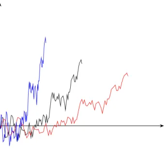
Lemma 4.4. (Scaling invariance) Suppose{B(t) :t ≥0} is a standard Brownian motion and let

a > 0. Then the (scaled) process {X(t) : t ≥ 0} defined by X(t) = 1_aB(a2t) is also a standard Brownian motion.

Proof. The only property that is not obvious to hold is that the distribution of increments is normally distributed and with the right parameters. Observe that:

X(t)−X(s) = 1

a(B(a

2_t₎₋_B₍_a2_s₎₎_,

which is a normal distribution with the parameters required for a standard Brownian motion, since it has expectation 0and variance _a12(a2t−a2s) =t−s.

This principle will be retrieved in the next chapter. To anticipate it, just consider T(a,b) =

inf{t ≥0 :B(t) =a orB(t) = b}, that is, T(a,b) is the first exit time of the interval [a,b] for a one-dimensional Brownian motion . Then, with the scaled Brownian motion X(t) = _a12B(a2t):

E(T(a,b)) =a2E infnt ≥0 :X(t) = 1 or X(t) =b a o =a2E T(1,b a) .

(22)

Figure 4.1: Brownian motion and scaled processes with parameters a=1.25anda=0.75

Lemma 4.5. Let{Bt :t ≥0} a standard Brownian motion. Then for all s <t:

Cov(Bs,Bt) =s

Proof. WriteBsBt =Bs2+Bs(Bt−Bs), then, using that their mean is 0:

Cov(Bs,Bt) =E(BsBt)−E(Bs)E(Bt) =E(Bs2)−E(Bs)E(Bt)

=_E(B_s2) =Var(Bs) +E(Bs)2 =s

since Bs ∼N(0,s) for anys ≤t and increments of non-overlapping intervals are independent.

Theorem 4.6. (Time inversion)Suppose{B(t) :t ≥0} is a standard Brownian motion, then the process {X(t) :t≥0} defined by:

X(t) = (

0 for t= 0

tB(1_t) for t6= 0 is also a standard Brownian motion.

Proof. {X(t) : t ≥ 0} is also a Gaussian process and the random vectors (X(t1), ... ,X(tn)) have

expectation 0. Using the previous lemma, covariance for h>0 is:

Cov(X(t+h),X(t)) = (t+h)CovB 1 t+h ,B1 t =t

Then, the covariance is also the one of a Brownian motion. Now, it only remains to see that paths are continuous. Away from the origin, they are clearly continuous. At t = 0, on the rationalsX is almost surely continuous on(0,∞), so:

lim

t→0X(t) = 0 almost surely

(23)

The inversion will be a very useful in the analysis of assymptotic properties of Brownian motion as it will suffice to study it in a neighbourhood oft = 0.

Corollary 4.7. Almost surely,

lim

t→∞

B(t)

t = 0.

Proof. Let{X(t) :t ≥0} be defined as in Theorem 4.6, then by continuity ofX(t):

lim t→∞ B(t) t = limt→∞X 1 t =X(0) = 0.

4.4 Nondifferentiability

The natural questions that arise at this point are mainly two:

i) How strong is the continuity of Brownian motion?

ii) Is Brownian motion more regular than continuous, i.e., it can be diferenciated at some points or almost surely every point is nondifferentiable?

This two question will be answered in this section. The second one will be answered in brief, whereas the first one will be quantified by the notion of α-Hölder continuity.

Definition 4.8. A function f : [0,∞)→R is said to belocally α-Hölder continuous atx ≥0, if there exists >0 andc >0such that

|f(x)−f(y)| ≤c|x−y|α, for all y≥0with |y−x|<

We refer to α >0 as theHölder exponent andc >0 as theHölder constant.

This is a measure on the strength of continuity of a function: as αincreases the continuity gets stronger. For the particular case of Brownian motion, α = 1₂ is the critical value, as the following result states. We do not give a formal proof of it, since it requires a previous theorem, but it can be found in detail in [8], when Brownian motion continuity is extensively discussed.

Proposition 4.9. If α < 1₂, then, almost surely, Brownian motion is everywhere locally α-Hölder continuous.

It is important to recall that α < 1₂ is the optimal result meaning that for larger values of

α > 1₂ the property does not holds, and there exist points where Brownian motion is not α-Hölder continuous, almost surely.

Next point to discuss is the differentiability of Brownian motion. Firstly, some local properties will be given, and then the nondifferentiability property will be extended to any compact set. Here, it will be fundamental to retrieve the inversion property of Brownian motion together with two new notions of derivatives.

(24)

Proposition 4.10. Almost surely, for all 0<a<b <∞, Brownian motion is not monotone on the interval [a,b].

Proof. Suppose[a,b]is an interval of monotonicity, i.e., B(s)<B(t) for alla <s <t <b. Then we can split the interval in a =a1 < a2 < · · · <an = b which are n subintervals of [a,b]. Then,

every incrementB(ai+1)−B(ai)has to have the same sign, as Brownian motion is monotone on the

interval. Also, increments are independent, hence the probability for all them to have the same sign is 2·2−n. Takingn → ∞, the probability of[a,b]of being an interval of monotonicity is 0. Taking countable unions gives us that there are no such intervals with rational endpoints, but any interval must contain rational numbers, so we have the result required.

Now, to continue studying the differentiability of Brownian motion, we are interested in its assymptotic behaviour, and then applying time inversion property, we will be able to deduce new properties for times neart = 0.

Proposition 4.11. Almost surely, lim sup n→∞ B(n) √ n = +∞ lim infn→∞ B(n) √ n =−∞

In order to prove this proposition, we need an auxiliary result: the Hewitt-Savage0−1 law for exchangeable events.

Definition 4.12. LetX1, ... ,Xn be a sequence of random variables in a probability space (Ω,F,P), and consider a set Asuch that:

{X1, ...Xn∈A} ∈ F

The event {X1, ...Xn∈A}is called exchangeable if

{X1, ...Xn∈A} ⊂ {Xσ1, ...Xσn ∈A}

for all finite permutations of N, i.e., permutations with a finite number of nonfixed elements (Note that the inclusion can eventually become an equalty, in some cases).

Plainly, an event is exchangeable if it is closed under permutations of random variables. For instance, in the exmaple below, if Brownian motion is condidered in the discrete version, i.e., as a random walk, it is clear that many paths lead to the same event at the n-th step, the only condition that they must share is that the number of up/down moves is equal. All events that share this condition are exhangeable. The following law was firstly introduced in [5]:

Lemma 4.13. (Hewitt-Savage 0−1 law)

Let be(Xn) a sequence of independent identically distributed random variables. Then theσ-field of

exchangable eventsE is trivial.

Proof. We need to prove that for any A ∈ E, P(A) is either 0 or 1. Take A ∈ E. Given a partition of the σ-field E =∪Fn, approximate A by An ∈ Fn such that P(A4An) → 0. We write

An ={(X1, ...Xn) ∈Bn} and A˜n={(Xn+1, ...X2n)∈Bn} and condider the permutation the sends

An to A˜n.

By exchangeability, P(˜An4A) = P(An4A) ⇒ P(An∩A˜n) → P(A). Since the sequence (Xn) is

(25)

Now, we have everything necessary to proof the non-differentiability, applying the Hewitt-Savage

0−1 law:

Proof. (Proposition 4.11) By Fatou’s lemma, we have:

P(B(n)>c

√

n infinitely often)≥lim sup

n→∞ P

(B(n)>c√n)>0

Taking Xn=B(n+ 1)−B(n), note that:

{B(n)>c√n infinitely often}={ n X j=1 Xj >c √ n infinitely often}

is an exhangeable event. Hence, by lemma 4.13 with probability1,B(n)>c√n infinitely often. As the constant c can be taken as large as desired, we deduce the first equalty of the proposition. The other part is proved analogously.

In Corollary 4.7 it has been proved that the local growth of Brownian motion is slower than a linear function. The Proposition 4.11 shows that the growth is larger than the square root, so it is natural to try to find an intermediate function that expresses the assymptotic growth of Brownian motion more accurately. The answer to this question will be given by the law of iterated logartihm, which will not be stated in this work, although more details can be found in [8].

Definition 4.14. Given function f, theupper derivative is defined by:

D∗f(t) = lim sup

h↓0

f(t+h)−f(t)

h

Analogously, the lower derivative:

D∗f(t) = lim inf

h↓0

f(t+h)−f(t)

h

Theorem 4.15. Fix t ≥ 0. Then, almost surely, Brownian motion B(t) is not differentiable at t. Furthermore,

D∗B(t) = +∞ andD∗B(t) =−∞

Proof. Given a standard Brownian motionB(t), we construct another by time inversion that satisfies:

D∗X(0)≥lim sup n→∞ X(1_n)−X(0) 1 n ≥lim sup n→∞ √ nX(1 n) = lim supn→∞ B(n) √ n = +∞.

Thus, X(t) is not differentiable at t = 0. Now, consider B(t) = X(t +s)−X(s), and given the non-differentiability ofX(t)att = 0, now it is equivalent to the nondifferentiability ofB(t)att.

From the theorem above we cannot still deduce the desired property, it is a weaker form of it. We know that for a given t, Brownian motion will be nondifferentiable, almost surely, but it is not equivalent that almost surely every point is a nondiferentiability point. There exists a subtile but important difference between both statements, due to quatificator orders. However, the second statement is proved in the next theorem.

(26)

Theorem 4.16. Almost surely, Brownian motion is nowhere differentiable. In addition, almost surely, for all t, either D∗B(t) = +∞ or D∗B(t) =−∞ or both.

Proof. Suppose there is t0 ∈[0,1]such that−∞<D∗B(t)<D∗B(t)<∞, then

lim sup

h↓0

|B(t+h)−B(t)|

h <∞.

By continuity of Brownian motion in the interval[0,T], we would have that:

sup

h∈[0,1]

|B(t+h)−B(t)|

h <M.

Whence it suffices to prove that this happens with zero probability. Take t0 ∈[k₂−n1,₂kn], for n >2

and 1≤j ≤2n−k, by the triangle inequalty:

B k+j 2n −Bk+j−1 2n ≤ B k+j 2n −B(t0) + B(t0)−B k+j −1 2n ≤M j 2n +M j −1 2n =M 2j + 1 2n .

Define the events

Ωn,k = n B k+j 2n −Bk+j −1 2n ≤M 2j + 1 2n forj = 1,2,3, ...l o .

Then by independence of marginal distributions of increments in a Brownian motion and properly scaling of the process:

P(Ωn,k) = l Y j=1 P n B k+j 2n −Bk+j−1 2n ≤M 2j+ 1 2n o ≤_P{|B(1)| ≤ √7M 2n} l_.

Now, we have to think accurately of the distribution of B(1). Note that we are considering a discrete approach of Brownian motion, i.e., a random walk. Then,B(1)con only take a finite number of values, following a binomial distribution. Thus, when n → ∞ by the central limit theorem A.12 the distribution tends to a N(0,1₄), thus:

P(|B(1)| ≤ 7M √ 2n) = Z √7M 2n −_√7M 2n 2 √ 2πe −x2 dx ≤ √7M 2n = 7M2 −n 2.

Hence, given n, we have:

P( 2n₋_l [ k=1 Ωn,k)≤2n(7M2− n 2)l <(7M)32− n 2,

given, l ≥3, which is necessary for this events to form a convergent sum for all n. Now, using the Borel-Cantelli lemma: P n there is t0∈[0,1] : sup h∈[0,1] |B(t0+h)−B(t0)| h ≤M o ≤_P 2n₋_l [ k=1

Ωn,k for infinitely many n

= 0,

where the inequalty holds as a consequence of the more restrictive condition, as for the latter case the condition must be satisfied infinitely many cases.

(27)

5. The Markov property of Brownian

mo-tion

The introduction made in chapter 3 will now be contextualized with Brownian motion. Some results seen there will be revisited, may be with some modifications, adapted to this particular process. It aims at stablishing the Markov property (weak and strong versions) using the notion of stopping times that holds for Brownian motion, and also some consequences will be included, such as the reflection principle.

5.1 Markov property and Blumenthal’s

0 −

1 law

In this chapter our mission is to state in which sense Markov property holds for the case of Brownian motion, even in multidimensional cases, and from here deduce some interesting properties and laws. In a more general property, we will see that some processes that proceed from Brownian motion are also Markov processes. This will lead to the reflection principle, which will be dicussed in the next section, whose consequences are surprinsing and interesting from a mathematical point of view.

Definition 5.1. IfB1, ...Bdare independent Brownian motions started in(x1, ... ,xd)T, the stochastic

process {B(t) :t ≥0} given by

B(t) = (B1(t), ... ,Bd(t))

is a d-dimensional Brownian motion started in(x1, ... ,xd)T.

If we recall the Markov property for a stochastic process, we have that a process{B(t) :t ≥0}

with such property is only determined by the distribution at some s, and information in the interval

[0,s]can be disregarded, and it will have no influence in the future of the process.

Also note that two stochastic processes{X(t) :t ≥0}and {Y(t) :t ≥0}are said to be inde-pendentis for any set oft1,t2,· · ·,tnands1,s2,· · · ,snthe random vectors(X(t1),X(t2), ... ,X(tn))

and (Y(s1),Y(s2), ... ,Y(sn))are independent vectors.

Theorem 5.2. (Markov property) Suppose that {B(t) : t ≥ 0} is a d-dimensional Brownian motion started in x ∈ _Rd_{. Let} _s _> ₀_{, then the process} _{_B₍_t₊_s₎₋_B₍_s_{) :} _t _≥ ₀_} _{is a standard}

Brownian motion independent of the process {B(t) : 0≤t≤s}.

Proof. It is clear that{B(t+s)−B(s) :t ≥0}satisfies the definition of ad-dimensional Brownian motion, and the independence of {B(t) : 0 ≤ t ≤ s} is a consequence of the independence of increments that characterizes the Brownian motion, by definition.

In this context, information that a random process gives us can be gathered in afiltration, which abstractly will come to express exactly this. More formally:

Definition 5.3. Afiltrationon a probability space(Ω,F,P)is a family(F(t) :t ≥0)ofσ-algebras such thatF(s)⊂ F(t)⊂ F ∀s <t. A prrbability space with a filtration defined, is called afiltered probability space. A stochastic process {X(t) : t ≥0} defined on (Ω,F,P) is called adapted if

X(t) isF(t)-measurable for anyt ≥0.

Remark 5.4. A filtrationF(t)can also be denoted byFt, which is generally used, but we will denote

it in the first way because the latter notation can result ambiguous for the next steps that we are going to consider in this chapter.

(28)

5 The Markov property of Brownian motion

Given a random process, such as Brownian motion{B(t) :t ≥0}, it is easy to build an adpated filtration. We just need to take the filtration(F0₍_t₎₎_{, where}_F0₍_t₎_{is the}_σ_{-algebra generated by the}

random variables {B(s) : 0≤s ≤t}. Obviously, Brownian motion is adpated to this filtration, that contains the information of the process observed up to t. From theorem 5.2 we can easily deduce that the process{B(t+s)−B(s) :t ≥0}is independent ofF0₍_s₎_{, but can this be extended? What}

if we know the information up to an infinitessimal time instant afters? Consider the filtration

F+(s) =∩t>sF0(t)

Then, clearly F0₍_s₎_{⊂ F}+₍_s₎

Theorem 5.5. For s ≥0, the process{B(t+s)−B(s) :t ≥0}is independent of F+₍_s₎_.

This theorem is just a consequence of the continuity of Brownian paths. It is necessary to take a decreasing sequence {sn}n≥0 convergent tos, and by continuity, the theorem holds.

From all σ-algebras, there is one, the so-called germ σ-algebra, defined as F+₍₀₎_{, which contains}

information known at an infinitessimal time after the start of the process. So, the following result was found and named after its discoverer in [3]:

Theorem 5.6. (Blumenthal’s 0−1 law) Let A∈ F+₍₀₎_{, then}

P(A)∈ {0,1}

Proof. Apply Theorem 5.5 for s = 0, which implies that for any A ∈ σ{B(t) : t ≥ 0}, A is independent of F+₍₀₎_{. In particular applies if} _A_{∈ F}+₍₀₎_{, whence}_A _{is independent of itself, thus}

P(A)∈ {0,1}

Remark 5.7. The previous proof is interesting from the point of view of the idea used. 0−1 laws have appeared in this work, and all of them are proved using the same idea. If an event A has probability either 0 or1, then it suffices to prove that this event is independent of itself.

Theorem 5.8. Suppose {B(t) :t ≥0}a standard Brownian motion. Defineτ =inf{t >0 :B(τ)>0} andσ=inf{t>0 :B(τ) = 0}. Then,

P{τ = 0}=P{σ = 0}= 1 Proof. {τ = 0}= ∞ \ n=1 n there is0< < 1 n :B()>0 o

Obviously, the event is in F+₍₀₎_{, and in addition,}

P(τ < t)>P(B(t) >0) = 1₂, which proves the first part, as a consequence of theorem 5.6. The same argument is valid for the case B(t) < 0, thus, by continuity of Brownian motion, using the mean-value theorem, we have that the property for σ holds.

5.2 The strong Markov property

As in chapter 3, to introduce the idea of the strong Markov property, it is necessary to use stop-ping times, which intuitively are related with the Markov property of only near-present dependence. Roughly, a stopping time is a random variable whose value at time t can be deduced from the information of the past values of itself. More formally,

Definition 5.9. A random variable T with values in [0,∞], defined in a probability space with an associated filtration (F(t) : t ≥0) is called astopping time if {T <t} ∈ F(t), for every t ≥0. Additionally, if {T ≤t} ∈ F(t) for everyt ≥0, then T is a strict stopping time.

(29)

From the definition is is clear that every strict stopping time is also a stopping time, just observing the following: {T <t}= ∞ [ n=1 {T ≤t+1 n} ∈ F(t).

The main problem is to indentify in which cases the converse in also true. Fortunately, there are nice enough filtrations where this happens. To overcome this problem in case of Brownian motion it is appropiate to work with the filtration (F+₍_t_{) :} _t _≥ ₀₎_{. Recall that this filtration satisfies} F0₍_s₎ _{⊂ F}+₍_s₎_{, what results in a larger filtration, and hence more stopping times accepted by}

the process. The key point why we consider this filtration instead of the natural one is due to the

right-continuity ofF+₍_t₎_.

Theorem 5.10. Every stopping timeT with respect to the filtration(F+₍_t_{) :}_t_≥₀₎_{is also a strict} stopping time.

For every stopping timeT, we define:

F+(T) ={A∈ A:A∪ {T <t} ∈ F+(t) for all t≥0}

This introduces a slightly different notion, as now we are only considering the events that are com-pletely known or determined up to a stopping time T.

Theorem 5.11. (Strong Markov property) For every almost surely finite stopping time T, the process {B(t+T)−B(T) :t≥0}is a standard Brownian motion independent of F+₍_T₎_.

Proof. We start by an upper discrete approximation of the stopping time T by Tn = (m₂+1)n if

m

2n ≤T <

(m+1)

2n . Also, consider the following processes:

Bk(t) =B t+ k 2n −Bk 2n

and, fixingn, consider:

Bn(t) =B(t+Tn)−B(Tn)

Suppose we have an event E ∈ F+₍_T

n). Then, for every event {Bn∈A}, we have:

P({Bn∈A} ∪E) = ∞ X k=0 P({Bk ∈A} ∩E∩ {Tn=k2−n}) (∗) = = ∞ X k=0 P({Bk ∈A})∩P(E ∩ {Tn=k2−n}) (∗∗) = =_P({B ∈A} ∞ X k=0 P(E ∩ {Tn=k2−n}) =P{B∈A}P(E)

which shows that Bnis a Brownian motion independent ofE, hence of F+(Tn). In the proof it has

been used that:

(*) {Bk ∈A} is independent of {E∩Tn=k2−n} ∈ F+(k2−n).

(*) P(Bk ∈A) =P(B ∈A) is independent of k.

The generalisation to stopping times T follows from the continuity of Brownian motion for any sequenceTn such thatTn↓T.

(30)

5.3 The reflection principle

The first and most important consequence of the Markov property of Brownian motion is thereflection principle. It is almost a raw application of it. We consider a stopping timeT, which can be arbitrary, and the process:

B∗(t) =B(t)1_{_t_≤_T_}+ (2B(T)−B(t))1_{_t_>_T_} (5.1) t B(t) B∗(t) a=B(T) T

Theorem 5.12. (Reflection principle) IfT is a stopping time and {B∗(t) :t ≥0} is a standard Brownian motion, then the process defined in ( 5.1), called Brownian motion reflected at T is also a standard Brownian motion.

Proof. IfT is finite, then using the strong Markov property,

{B(t+T)−B(T) :t ≥0} and {−(B(t+T)−B(T)) :t≥0}

are Brownian motion independent of the original {B(t) : t ≥ 0}. Hence the process B∗(t) is a standard Brownian motion, as the first part and the second one have the same distirbution and both are standard Brownian motions.

Leta=B(T), that is, the level at the stopping time. This level clearly exhibits a symmetry for those Brownian motions that att ∈[T,T0]are above or belowa, as for any path that is above there is a relfected path that is below and conversely.

Let M(t) = max

0≤s≤tB(s). This random variable has unknown distribution, a priori, but in application

of the reflection principle, we can determine it:

Corollary 5.13. Ifa>0, thenP{M(t)>a}= 2P{B(t)>a}

Proof. LetT =inf{t ≥0 :B(t) =a}and{B∗(t) :t ≥0}is the refelected Brownian motion, then:

P(M(t)>a) =P(M(t)>a,B(t)≥a) +P(M(t)>a,B(t)<a) =

P(B(t)>a) +P(B∗(t)>a) = 2P(B(t)>a)

since both are Brownian motions.

In chapter 4 the regularity of Brownian motion have been studied with a direct approach. Now, also as a consequence of the reflection principle, the non-differentiation results is retrieved.

(31)

Corollary 5.14. If{B(t) : 0≤t ≤T} is a standard Brownian motion, then, almost surely, ∀t ≥0

B(t) is nondifferentiable.

Proof. We argue by contradiction. Suppose that at somet, the derivative exists. Then:

|B(t+0)−B(t)| ≤A Let M() =max 0 |Bt+ 0 −B_t| ≤A. By Corollary 5.13, we have P(M(t)> A) = 2P(B()> A) = 2P(N(0,)> A) = 2P(N(0,1)>√A)−→ →0 1

where N denotes a normal distribution.

Thus, there is a contradiction, since the maximum is not bounded for any with probability1, and therefore,B(t) is nondifferentiable at any point.

(32)

6. From random walks to Brownian

mo-tion

6.1 Preliminaries

Throughout this chapter, there will be a permanent idea overflying theorems and arguments: how to approximate a Brownian motion through a random walk. There are many constructions possible, but the approach given in the proof of the Ray-Knight theorem has the advantadge that it is natural and elementary. Sometimes, the embedding process is called twist and shrink for obvious reasons. The key point is to construct a sequence of random walks uniformly convergent to Brownian motion.

Firstly, imagine that we observe the motion of a particle when it hits to coordinates {j,j ∈_Z}. Then, we observe the particle exclusively when coordinates {₂j,j ∈ _Z} are hit. And so on. This generates a sequence of random walks, which suitably managed, converge appropiately.

We consider a sequence of independent identically distributed random variablesXm(k)in a probability

space (Ω,F,P) such that P(Xm(k) = ±1) = 1₂, for m ≥ 0 and k ≥ 1. Then the random walk

considered is: Sm(0) = 0 and Sm(n) = Pnk=1Xm. Thus, E(Xm(k)) = 0 and Var(Xm(k)) = 1.

Hence:

E(Sm(n)) = 0 Var(Sm(n)) =n. (6.1)

This expression suggests that time and space scaling can not be done arbitrarely. The question is: if the space is halved, what should be time reduction in order to converge to a Brownian motion? From (6.1), we know that the square root of the average squared distance of a random walks from the origin at timen is√n, so an appropiate shrink aftern would require a lenght of √1

n.

So far, the construction of the random walks is independent ofm, but this does not give a convengence to a limit as desired. We need to find a link, which will be a successive refinement of them, that joins them correctly. With this construction in mind, we define thestopping times Tm(0) = 0, and:

Tm(k+ 1) =inf{n>Tm(k) :|Sm(n)−Sm(Tm(k))|= 2} (6.2)

These are random (stopping) times when the random walk visits even integers different from the provious one. A key point is that the distribution of Tm(k) is known, and it is given by the following

Lemma:

Lemma 6.1. LetTm(k)be random variables defined as in (6.2). ThenTm(k)follows the distribution

of the double negative binomial random variable with parameters k and p= 1₂.

Proof. Consider the random variables τj = inf{n > τj−1 : |Sm(n)−Sm(τj−1)| = 2} −τj−1, with τ0 = 0. These random variables have a known distribution. Imagine the random walks as a sequence

of independent pairs of steps: returnsor change of magnitud ±2. Then, P{τk+1 = 2j}= ₂1j, what

implies thatτk+1= 2Yk+1, whereYk+1 is a geometric random variable with paraemterp = 1₂. This

results follow from the fact that Tm(k)can be seen as the sum of k independent geometric random

variables τj: Tm(k) = k X j=0 τj = 2 k X j=0 Yj,

that leads to a negative binomial distribution, and also, E(Tm(k)) = 4k and Var(Tm(k)) =

4 p

(33)

6 From random walks to Brownian motion

As a consequence the Central Limit Theorem 6.1 and A.12, we have that for any real fixed x and

k → ∞:

PnTk√−4k 8k

o

→Φ(x) (6.3)

where Φ(x) denote the cummulative distribution of a standard normal random variable. Now, we can define recursively twisted random variables forTm(k)<n<Tm(k+ 1):

˜ Xm(n) = ( Xm(n) if Sm(Tm(k+ 1))−Sm(Tm(k)) = 2 ˜Xm−1(k+ 1) −Xm(n) otherwise (6.4) and then S˜m(n) =Pjn=1X˜m(j). 1 2 1 2 3 u u u u Figure 6.1: S0(t,ω) −2 2 1 5 10 15 u u u u Figure 6.2: S1(t;ω) −2 2 4 6 T1(1)T1(2) T1(3) u u u u Figure 6.3: S˜1(t;ω)

The figures below illustrate thetwistintroduced to the random walks that correlate two consec-utive terms of the sequence. However, this correlation must satisfy some restrictions, commented above, and next Lemma is going to give us certainty that the construction respects the random walk structure.

Lemma 6.2. For eachm≥0,S˜(t),(t ≥0)is a random walk, that is,X˜m(1),X˜m(2), ... is a sequence

of independent random variables indentically distributed such that:

P{X˜m(n) = 1}=P{X˜m(n) =−1}=

1

2 (6.5)

The proof of this lemma is ommited, since its very extense. The difficult point of it is to prove the independence of the random walks defined. For more detials, see [9, Lemma 1].

(34)

6 From random walks to Brownian motion

6.2 Twist and shrink embedding

The main consequence of Lemma 6.2 is the twistproperty that implies the correlation between two consecutive random walks in the following way:

˜ Sm(Tm(k)) = k X j=1 (˜Sm(Tm(j))−S˜m(Tm(j −1))) = k X j=1 ˜ Xm−1(j) = ˜Sm−1(k) (6.6)

The next step is the shrink of the random walk. We know that time steps must be the square of spatial steps. Therefore, we define them-th approximation to the Wiener process by:

˜ Bm t 22m = 1 2mS˜m(t) (t≥0,m≥0) (6.7)

Rewriting it with a change of variable:

˜

Bm(t) = 2−mS˜m(22mt)

These expressions for (m ≥ 0) give an approximation to the Wiener process on the coordinates

x = ₂jm j ∈ Z. Thus, for the case of Brownian motion, (6.6) becomes the following refinement

property: ˜ Bm T_m(k) 22m = 1 2mS˜m(Tm(k)) = 1 2mS˜m−1(k) = ˜Bm−1 k 22(m−1) (6.8) for anym≥1 andk ≥0.

The main objective of this chapter is to see how, from the refinement property proved above, the times Tm(k)

22m and ₂2(mk−1) get arbitrarely close, so that, Bm(t) converges to the Wiener process,

donoted byW(t), hereinafter. Firstly, we establish a technical lemma, which will be useful for other auxiliar results.

Lemma 6.3. Suppose that forj ≥0, we haveE(Zj) = 0 andVar(Zj) =j and with somea>0and

b >0,

P({|Zj| ≥t})≤2aje−bt (t ≥0)

(exponential-Chebyshev inequalty).

Assume as well that there exists j0 >0 such that for anyj >j0,

Pn|√Zj|

j >xj

o ≤e−xj2

whenever Xj → ∞ andxj =o(j1/6) (large deviation type inequalty).

Then, for any C >1,

Pn max 0≤j≤N|Zj| ≥(2CNlog(N)) 1 2 o ≤ 2 N1−C (6.9) if N is large enough,N ≥N0(C).

Proof. Firstly we introduce a bound for the maximum, which, although is not accurate, can be very useful in this lemma. For any random variable Zj, it holds that:

P( max 1≤j≤NZj >t) =P(∪ N j=1{Zj >t})≤ N X j=1 P{Zj >t} (6.10)

Brownian motion: a random walk approximation

Title:

Author:

Advisor:

Department:

Academic year:

Degree in Mathematics

Universitat Politècnica de Catalunya

Facultat de Matemàtiques i Estadística

Degree in Mathematics

Bachelor’s Degree Thesis

Brownian motion: a random walk

approximation

Sergio Gutiérrez Moya

Supervised by Oriol Serra Albó

June, 2018

Abstract

Contents

1. Introduction

2. Overview of Stochastic Processes

3. Markov chains

3.1 Discrete-time Markov Chains

3.2 Hitting times, recurrence and transience

3.3 Random Walks

4. Introduction to Brownian motion

4.1 A joint probabilities approach. The Wiener process

4.2 Wiener’s theorem

4.3 Time scaling and time inversion

4.4 Nondifferentiability

5. The Markov property of Brownian

mo-tion

5.1 Markov property and Blumenthal’s

0

−

1

law

5.2 The strong Markov property

5.3 The reflection principle

6. From random walks to Brownian

mo-tion

6.1 Preliminaries

6.2 Twist and shrink embedding