Application of Modern Fortran to Spacecraft Trajectory Design
and Optimization
Jacob Williams∗ ERC Inc., Houston, TX, 77058
Robert D. Falck†
NASA Glenn Research Center, Cleveland, OH, 44135
Izaak B. Beekman‡
ParaTools Inc., Baltimore, MD, 21228
In this paper, applications of the modern Fortran programming language to the field of spacecraft trajectory optimization and design are examined. Modern Fortran (the latest stan-dard is Fortran 2008, and the newer Fortran 2018 stanstan-dard is due to be published next year) is a significant enhancement to the classical Fortran 77 language. Modern object-oriented Fortran has many advantages for scientific programming, although many legacy Fortran aerospace codes have not been upgraded to use the newer standards (or have been rewritten in other languages perceived to be more modern). NASA’s Copernicus spacecraft trajectory optimiza-tion program, originally a combinaoptimiza-tion of Fortran 77 and Fortran 95, has attempted to keep up with modern standards and makes significant use of the new language features. Various algorithms and methods are presented from trajectory tools such as Copernicus, as well as modern Fortran open source libraries and other projects.
I. Introduction
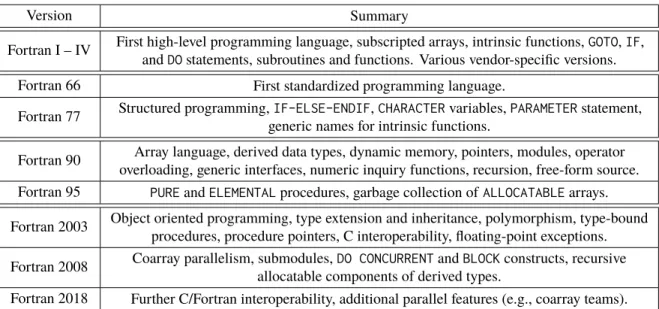
The original version of Fortran, developed by IBM in the late 1950s, was the first high-level programming language. It has continued to be updated regularly up to the present day. A brief overview of the Fortran language evolution is summarized in Table 1. For more details, see References [1–3]. The “classical” version of the language was first standardized in Fortran 66 and updated in Fortran 77. Significant expansions of the language were implemented in Fortran 90 and Fortran 2003. Fortran 2003 [4] was a very significant update that made Fortran an object-oriented language (the difference between Fortran 2003 and Fortran 77 is akin to the difference between C++ and C). The latest standard is Fortran 2008 [5], the upcoming Fortran 2018 standard (formerly known as Fortran 2015) [6] is due to be published next year, and planning has begun for the next standard (Fortran 202x). Fortran has maintained a high degree of backward compatibility, with each revision being mostly a superset of the previous revision (so older code can still be compiled with a modern compiler). The term “modern Fortran”, as used in this paper, is intended to mean Fortran 2003 (and later), and implies free-form source, thread-safety, object-oriented (where appropriate), clearly written and well-documented code.
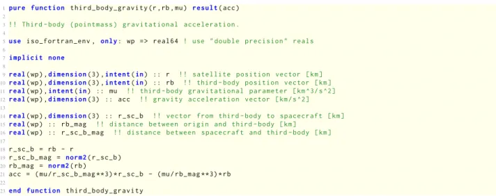
Fortran is a high-level general purpose programming language very well suited for scientific, technical and high performance computing (HPC) [7–10]. The syntax is fairly intuitive and includes built-in vector and matrix handling features, with less necessity than C-based languages to use potentially unsafe pointers, which lends itself to vectorization and parallelization. As an example, a basic Fortran function for computing third-body gravitational acceleration [11] is shown in Fig. 1. This function highlights the straightforward “close to the math” syntax of the language, including operations involving vectors, without the need for external libraries. The language also includes advanced high-level object-oriented features which are critical for the development of very complex codes. A standardized interoperability with the C programming language also allows Fortran to call C and for C to call Fortran, opening up the language to other libraries not written in Fortran (note that interoperability with C also means interoperability with any language that is also interoperable with C, such as C++ and Python).
∗Senior Astrodynamics Engineer, JETS Engineering Department, AIAA Senior Member †Aerospace Engineer, Mission Analysis and Architecture Branch, AIAA Member ‡HPC Scientist, AIAA Member
1pure f u n c t i o n third_body_gravity (r,rb ,mu) r e s u l t(acc)
2
3!! Third - body ( pointmass ) gravitational acceleration . 4
5use iso_fortran_env , only: wp => real64 ! use " double precision " reals
6
7i m p l i c i t none
8
9real(wp),d i m e n s i o n(3) ,i nt e n t(in) :: r !! satellite position vector [km]
10 real(wp),d i m e n s i o n(3) ,i nt e n t(in) :: rb !! third -body position vector [km]
11 real(wp),i n t e n t(in) :: mu !! third - body gravitational parameter [km ^3/s^2]
12 real(wp),d i m e n s i o n(3) :: acc !! gravity acceleration vector [km/s^2]
13
14 real(wp),d i m e n s i o n(3) :: r_sc_b !! vector from third - body to spacecraft [km]
15 real(wp) :: rb_mag !! distance between origin and third - body [km]
16 real(wp) :: r_sc_b_mag !! distance between spacecraft and third -body [km]
17
18 r_sc_b = rb - r
19 r_sc_b_mag = norm2( r_sc_b )
20 rb_mag = norm2(rb)
21 acc = (mu/ r_sc_b_mag **3) * r_sc_b - (mu/ rb_mag **3)*rb 22
23 end f u n c t i o n third_body_gravity
Fig. 1 Example Fortran Function to Compute Third-Body Gravity (from the Fortran Astrodynamics Toolkit).
This function highlights the “close to the math” syntax of Fortran, without the need to use external libraries. It has vector inputs and returns a vector output. The function is “pure” meaning that it has no side effects, which can allow the compiler greater possibilities for code optimization.
While there is a great deal of very high-quality freely available or open source Fortran 77 legacy code in existence (e.g., MINPACK, SLATEC, and MATH77 at Netlib∗), it is not in a form that is very appealing to modern programmers. For well documented third-party libraries that do not need to be changed, this obsolescence is not really an issue, but it can present severe impediments if the legacy code needs to be modified. Sometimes, refactoring is quite straightforward and enables many improvements to the original code. Recent activities including the development of new open source modern Fortran libraries hosted on sites such as GitHub, are a cause for optimism for the future of the language. In the aerospace field, for example, the Fortran Astrodynamics Toolkit (a work in progress) is intended to be a modern open source library for the foundational algorithms of orbital mechanics†.
The Copernicus spacecraft trajectory optimization program [12], developed at the Johnson Space Center (JSC) and distributed under a government use license‡, is an example of an actively-developed modern Fortran application. Copernicus is capable of solving a wide range of trajectory design and optimization problems, including trajectories centered about any planet or moon in the solar system, trajectories influenced by two or more celestial bodies such as halo orbits or distant retrograde orbits, Earth-Moon and interplanetary transfers, asteroid and comet missions, and more. One of the core elements of the program is the “segment”, which is the fundamental building block of mission design in Copernicus. Copernicus includes a full-featured Graphical User Interface (GUI) with interactive 3D graphics. The system is very flexible and has been used extensively at JSC (and other NASA centers) for a wide range of projects.
At NASA in general, many spacecraft trajectory optimization problems are solved using Fortran tools such as SORT [13], OTIS [14], MALTO [15], Mystic [16], and Copernicus. Other historic Fortran 77 tools have been replaced or rewritten in other programming languages. Examples include POST [17] (converted to C in the 1990s) and DPTRAJ/ODP (replaced with the C++/Python MONTE [18]). The JPL tool CATO [19] uses an “object-based” approach with Fortran 95, which is similar in some ways to how Copernicus was originally coded in the early-2000s. Unlike many of the legacy tools, the Copernicus code base (originally a combination of Fortran 77 and Fortran 95) has been kept up to date using modern Fortran features, including the incorporation of object-oriented design patterns [20]. This paper describes some of these modern Fortran concepts and their usefulness in trajectory design tools such as Copernicus.
∗Netlib Repository.http://www.netlib.org
†A Modern Fortran Library for Astrodynamics.https://github.com/jacobwilliams/Fortran-Astrodynamics-Toolkit ‡Copernicus Trajectory Design and Optimization System (Version 4.x).https://software.nasa.gov/software/MSC-25863-1
Table 1 Major Fortran Language Milestones.
Version Summary
Fortran I – IV First high-level programming language, subscripted arrays, intrinsic functions,GOTO,IF, andDOstatements, subroutines and functions. Various vendor-specific versions.
Fortran 66 First standardized programming language.
Fortran 77 Structured programming,IF-ELSE-ENDIF,CHARACTERvariables,PARAMETERstatement, generic names for intrinsic functions.
Fortran 90 Array language, derived data types, dynamic memory, pointers, modules, operator overloading, generic interfaces, numeric inquiry functions, recursion, free-form source. Fortran 95 PUREandELEMENTALprocedures, garbage collection ofALLOCATABLEarrays. Fortran 2003 Object oriented programming, type extension and inheritance, polymorphism, type-bound
procedures, procedure pointers, C interoperability, floating-point exceptions. Fortran 2008 Coarray parallelism, submodules,DO CONCURRENTandBLOCKconstructs, recursive
allocatable components of derived types.
Fortran 2018 Further C/Fortran interoperability, additional parallel features (e.g., coarray teams).
II. Survey of Algorithms
In the following sections, various algorithms and codes are discussed, along with examples of how they are implemented and used in modern Fortran. The focus is on high-level, object-oriented algorithms that are used in trajectory design tools such as Copernicus. Many of the codes discussed here are open source, and the links are given in footnotes for reference.
A. JSON
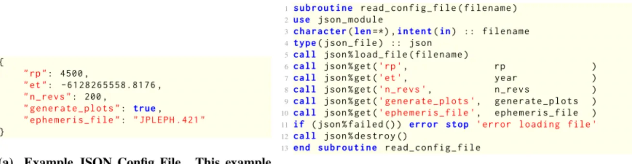
While the Fortran language does include facilities for reading and writing text and binary files, the only high-level text file format built into the language is known as a “namelist”. Many legacy codes use this format for input configuration files. Namelists are simple to read and write from Fortran code but have very severe limitations (such as limited error checking ability and strict variable type requirements). For modern applications, it is preferable to use a more standardized and flexible format with a high-level interface. JavaScript Object Notation (JSON) is a lightweight human-readable data exchange format that has a modern Fortran open source interface known as JSON-Fortran§. JSON can be used for configuration input files and data output files, as well as for communication between tools. Recent versions of Copernicus use JSON-Fortran for interfacing with user-defined plugins using a JSON-based application programming interface (API). An example of reading a JSON input file is shown in Fig. 2 using the high-level
json_fileclass. Methods exits in the class for retrieving data from a file, inquiring about the contents of the file or the types and sizes of individual variables, and error checking. In the example shown in Fig. 2b, theget()method, which is overloaded for integer, real, character, and logical scalar and vector variables, is used to retrieve values from the file. Other methods are also included for creating and modifying a JSON file.
In a future release, the main Copernicus input file format will transition from namelists to JSON. The JSON format allows for portable storage of arbitrary data, and the flexibility of the JSON-Fortran API will eliminate various limitations in the program that exist due to the rigidity of the namelist format. The ubiquity of JSON also provides opportunities for scripting Copernicus (and interfacing with plugins) in a variety of programming languages (such as Python). The JSON-Fortran API can also be used for general-purpose collection of data internally that can then be transformed into a variety of other formats. Copernicus employs this strategy to generate data output files in a variety of different formats (e.g., CSV, HDF5, and SPK).
A variety of other file formats is also available for use in modern Fortran codes via other third-party libraries, including INI¶, CSV‖, and HDF5∗∗.
§JSON-Fortran: A Fortran 2008 JSON API.https://github.com/jacobwilliams/json-fortran ¶Fortran INI ParseR and Generator.https://github.com/szaghi/FiNeR
‖Read and Write CSV Files Using Modern Fortran.https://github.com/jacobwilliams/fortran-csv-module ∗∗Object Oriented Fortran HDF5 Module.https://github.com/rjgtorres/oo_hdf
1{ 2 "rp": 4500 , 3 "et": -6128265558.8176 , 4 " n_revs ": 200 , 5 " generate_plots ": true, 6 " ephemeris_file ": " JPLEPH .421 " 7}
(a) Example JSON Config File. This example contains a hypothetical set of input parameters.
1s u b r o u t i n e read_config_file ( filename )
2use json_module
3c h a r a c t e r(len=*) ,i nt e n t(in) :: filename
4type( json_file ) :: json
5call json% load_file ( filename )
6call json%get('rp ', rp )
7call json%get('et ', year )
8call json%get('n_revs ', n_revs )
9call json%get('generate_plots ', generate_plots )
10 call json%get('ephemeris_file ', ephemeris_file )
11 if ( json % failed ()) error stop 'error loading file '
12 call json% destroy ()
13 end s u b r o u t i n e read_config_file
(b) The Code to Read the Example JSON File.
Fig. 2 Reading a config file using the JSON library is fairly straightforward. Additional error checking can be
done to check if each variable is found in the file and to verify the variable type (two features that are not easily done using Fortran namelists).
B. Dynamic Structures & Linked Lists
One of the limitations of Fortran 77 was the lack of any facility for creating and manipulating dynamic data structures. This was a significant impediment to the creation of very complicated interactive applications. Modern Fortran includes two components to facilitate dynamic data: allocatableandpointervariable attributes [2]. Both have their uses. Allocatable arrays are generally more efficient since they are guaranteed to be contiguous in memory, whereas pointers are allowed to point to non-contiguous array slices. Improper use of pointers can also lead to memory leaks, whereas allocatables will always be automatically “garbage collected” by the compiler when they go out of scope. A derived type can include an allocatable or pointer instance of the same type, thus allowing for the creation of many kinds of dynamic and recursive structures.
There are many example use cases for dynamic data structures in complex trajectory design software such as Copernicus. A primary example is the construction of the mission segments when reading the input file. A very simple example JSON snippet is shown in Fig. 3a, which could represent the initial conditions of a Copernicus segment (in this case, the initial timet0of the “coast” segment is inheriting the final timetf from segment 1, whereas other variables∆t
andx0are specified as real values). Data of this sort can be represented as a dictionary type structure containing integers,
reals, booleans, strings, and other dictionary instances, as shown in Fig. 3b. In an interactive tool like Copernicus, the data layout of the mission can change during run time (for example, when a new segment is inserted, or if the selected gravity model is changed in a segment). Lists of different types of complex objects have many other applications in trajectory software (including frames, celestial bodies, and gravity models).
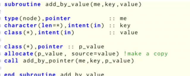
One of the basic building blocks of dynamic data structures is a linked list [21]. In earlier versions of Fortran, various workarounds were necessary to enable the creation of code to handle “generic” linked lists (i.e., a structure that can contain data ofanytype) [22]. The “unlimited polymorphic” variables introduced in Fortran 2003 make the creation of such structures much more straightforward (as shown in Fig. 4). Fig. 4a shows an example of a type that can be used to construct a polymorphic dictionary type structure using linked lists††. Here, the node content (value) is an unlimited polymorphic (class(*)) pointer variable, which can be allocated at run time to any variable type. Thekeyis also polymorphic (e.g, to allow for integer, string, or other types of keys). Using these concepts, the data structure shown in Fig. 3 can be built as a polymorphic linked list using the code shown in Fig. 4d. There are a variety of flavors of this technique that can be used to build and manipulate various dynamics structures such as lists, stacks, and queues. It is important to note that a linked list constructed using pointer allocations in this manner must be properly destroyed in order to avoid memory leaks (the structure must be traversed and the pointers deallocated). The compiler will not do this automatically. Typically, a linked list could be encapsulated into alistderived type that includes all the public methods for creating and manipulating the data, which may not require the caller to use pointer variables (this is done in the JSON-Fortran library). Thelisttype could also include a finalizer (a destructor-like type bound procedure called automatically when the variable goes out of scope) to clean up the memory. Dynamic structures using recursive allocatable variables are also possible (starting in Fortran 2008), which would be more memory safe, but perhaps less flexible depending on the use case [2].
1{ 2 " name ": " coast ", 3 "t0": { 4 " inherit ": { 5 " segment ": 1, 6 " node ": "TF" 7 } 8 }, 9 "dt": 1.0 , 10 "x0": 1000.0 11 }
(a) JSON Representation of Input Data. This is the type of data that could be read from a config-uration input file.
'name' → 'coast'
'dt' → 1.0
'x0' → 1000.0
't0' → 'inherit' → 'segment' → 1
'node' → 'TF'
(b) Linked List Representation of the Same Data.
Fig. 3 Example of Dictionary Type Structure. Using pointers, a variety of data structures can be created in
Fortran. The example here is similar to the type of information read from a Copernicus input file.
1type :: node
2 p r i v a t e
3 class(*) ,a l l o c a t a b l e :: key
4 class(*) ,p o i n t e r :: value => null()
5 type( node ),p o i n t e r :: next => null()
6 type( node ),p o i n t e r :: previous => null()
7 type( node ),p o i n t e r :: parent => null()
8 type( node ),p o i n t e r :: head => null()
9 type( node ),p o i n t e r :: tail => null()
10 end type node
(a) A Node in a Linked List. This type can be used to build tree structures. Both thekey andvalueare unlimited polymorphic variables.
1s u b r o u t i n e add_by_value (me ,key , value )
2 3type( node),p o i n t e r :: me 4c h a r a c t e r(len=*) ,i n t e n t(in) :: key 5class(*) ,i n t e n t(in) :: value 6 7class(*) ,p o i n t e r :: p_value
8a l l o c a t e(p_value , source = value ) !make a copy
9call add_by_pointer (me ,key , p_value )
10
11 end s u b r o u t i n e add_by_value
(b) Procedure for Adding a Node to a Linked List (by Value). In this method, the value is cloned using an
allocatestatement, which makes a copy to store in the list.
1s u b r o u t i n e add_by_pointer (me ,key , value )
2 3type( node),p o i n t e r :: me 4c h a r a c t e r(len=*) ,i nt e n t(in) :: key 5class(*) ,p o i n t e r :: value 6 7type( node),p o i n t e r :: p 8
9if (a s s o c i a t e d(me%tail )) then ! insert at end
10 a l l o c a t e(me%tail% next )
11 p => me% tail %next 12 p% previous => me%tail 13 else ! first item in the list
14 a l l o c a t e(me%head)
15 p => me% head 16 end if
17 me%tail => p 18 p% parent => me
19 a l l o c a t e(p%key , source =key) ! the key
20 p% value => value ! the value 21
22 end s u b r o u t i n e add_by_pointer
(c) Procedure for Adding a Node to a Linked List (by Pointer). In this case, the pointer is directly added to the list and no copy is made.
1p r o g r a m example 2 3use linked_list_module 4 5i m p l i c i t none 6
7type(node),p o i n t e r :: list
8type(node),p o i n t e r :: inherit
9class(*) ,p o i n t e r :: p_inherit
10
11 a l l o c a t e(list)
12 call add_by_value (list ,'name ','coast ')
13 call add_by_value (list ,'dt ',1.0 _wp)
14 call add_by_value (list ,'x0 ',1000.0 _wp)
15
16 a l l o c a t e( inherit )
17 call add_by_value (inherit ,'segment ',1)
18 call add_by_value (inherit ,'node ','TF ')
19 p_inherit => inherit
20 call add_by_pointer (list ,'t0 ',p_inherit )
21
22 end p r o g r a m example
(d) Constructing a Linked List. This is the data from Fig. 3, constructed as a linked list ofnodepointers.
Fig. 4 Linked List Example. A data type that contains pointers to instances of the same type can be used to
construct a variety of different types of data structures using linked lists. Thenextandpreviouspointers can
be used to build doubly-linked lists, while theparent,head, andtailpointers can be used for trees. See the
Mission Attribute Segment Plugin Internal Parser External DLL Script
Fig. 5 Class Hierarchy of Copernicus Mission Attributes. Abstract types are italicized, which exist only to be
extended. A mission consists of segments and plugins (either parser, DLL, or script).
1type,abstract,p u b l i c :: mission_attribute
2c o n t a i n s
3p r o c e d u r e( prop_func ),d e f e r r e d :: propagate
4end type mission_attribute
5
6type,e x t e n d s( mission_attribute ),p u b l i c :: segment
7c o n t a i n s
8p r o c e d u r e :: propagate => propagate_segment
9end type segment
10
11 type,e x t e n d s( mission_attribute ),abstract,p u b l i c ::
plugin 12 end type plugin
13
14 type,e x t e n d s( plugin ),abstract,p u b l i c ::
internal_plugin 15 end type internal_plugin
16
17type,e x t e n d s( plugin ),abstract,p u b l i c ::
external_plugin 18end type external_plugin
19
20type,e x t e n d s( internal_plugin ),p u b l i c :: parser_plugin
21c o n t a i n s
22p r o c e d u r e :: propagate => propagate_parser_plugin
23end type parser_plugin
24
25type,e x t e n d s( external_plugin ),p u b l i c :: script_plugin
26c o n t a i n s
27p r o c e d u r e :: propagate => propagate_script_plugin
28end type script_plugin
29
30type,e x t e n d s( external_plugin ),p u b l i c :: dll_plugin
31c o n t a i n s
32p r o c e d u r e :: propagate => propagate_dll_plugin
33end type dll_plugin
Fig. 6 High-Level Mission Attribute Definitions. All concrete mission attribute types (which are all derived
from the rootmission_attributestype) must define apropagate()method. For segments, this will integrate
the segment fromt0totf. For plugins, this could be as simple as evaluating one user-defined equation. See also
Fig. 5.
C. Copernicus Mission Attributes
A spacecraft trajectory optimization problem in Copernicus is constructed using two types of mission attributes:
segmentsandplugins(see Fig. 5). Segments are the original built-in mission components, which can represent a thrusting or coasting period, can include impulsive∆v maneuvers, and can represent any number of different vehicles [12]. Plugins are a recent addition to Copernicus, and allow for user-defined algorithms to be included in the mission and optimization problem [23]. Various types of plugins are available, as shown in Fig. 5. Copernicus also includes the concept ofgroups, which are collections of segments and/or plugins that define a specific optimization problem (a mission can include any number of groups). An outline of the basic code definitions for segments and plugins is shown in Fig. 6. The mission attributes use various object-oriented concepts including polymorphism, inheritance, encapsulation, and data hiding. Anabstractmission_attributetype exists only to be extended (variables cannot be declared of an abstract type). An abstract type may contain procedures that must be defined in the extended types (for example the
segmentstype). In the case of Copernicus mission attributes, each mission component defines apropagate()method (among others). Simulating the entire mission involves calling thepropagate()method of each mission attribute. D. Topological Sorting
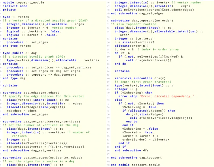
A Copernicus mission composed of many segments and plugins can contain complex interdependencies. The diagram in Fig. 7 shows a representation of the dependencies among the numerous segments and plugins of the Orion EM-1 [24] mission, which was designed in Copernicus. A complex mission can include hundreds or even thousands of segments. To avoid forcing the user to define the segments in a specific order, Copernicus employs a topological sorting algorithm to determine the order in which they must be propagated (for example, when computing the gradients). Topological sorting is a recursive algorithm used to determine the order in which a series of interdependent tasks must be completed [21]. A simple example of this algorithm is shown in Fig. 8, and an example use case is shown in Fig. 9. In this example, elements of a mission are numbered[1,2, . . .]. Their dependencies are known (for example,
S1 S2 S3 P1 S4 S5 S6 S7 S8 S9 S10 S11 S12 S13 S14 S15 S16 S17 S18 S19 S20 S21 S22 S54 P3 S23 S55 S24 S25 P4 S26 S27 S28 S29 S30 S31 S32 S33 S34 S35 S36 S37 S38 S39 S40 S41 S42 S43 S44 S45 S46 S47 S48 S49 S50 S51 S52 S53 S56 S57 S58 S59 S60 S61 S62 S63 S64 S65 S66 S67 S68 S69 S70 S71 S72 S73 S74 S75 S76 S77 S78 S79 S80 S81 S82 S83 S84 P2
Fig. 7 Copernicus Mission Dependency Diagram. The dependencies of the attributes of a mission can be
represented as a Directed Acyclic Graph (DAG). Copernicus dependencies arise, for example, when a segment inherits data from other segments. Before a segment (or plugin) can be propagated, all of its dependencies must be met (i.e., the segments it depends on must already have been propagated).
element 3 depends on elements 1 and 5). Thedag%toposort()method produces the order: [1,2,5,3,4], which is a valid propagation order that ensures that no segment is propagated before its dependencies are met. Another use of topological sorting in Copernicus is to ensure that a set of interdependent parser equations is evaluated in the correct order [23].
E. Calculation Expression Parser
General trajectory optimization tools such as OTIS and Copernicus allow users a great degree of freedom in defining their optimization problems. Much of this freedom comes from allowing the user to form their own objective functions and constraints as mathematical expressions based on an internal data dictionary of common variables and some available set of mathematical functions. Allowing the user to define these routines at run-time in infix notation extends the capability of such programs without the need to recompile the source code.
In this section, the implementation of a calculation expression parser is discussed. This parser converts mathematical expressions from infix notation into binary syntax trees. This parsing of mathematical expressions is a recursive operation, since expressions may be embedded in other mathematical expressions by wrapping them in parentheses. The parser uses several capabilities of modern Fortran to construct binary trees, which may then be efficiently evaluated.
1. Binary Syntax Trees
Binary syntax trees provide a data structure that can be used to represent complex mathematical expressions. As the name implies, a binary tree can have up to two children. Each node can represent a mathematical operator, function, literal numeric value, or variable value. The children represent arguments of operators or functions. Despite being limited to only two arguments, this framework accommodates most functions and operators commonly used. The algorithm presented here can be extended to a logicalif function withandandoroperators by allowing for a third
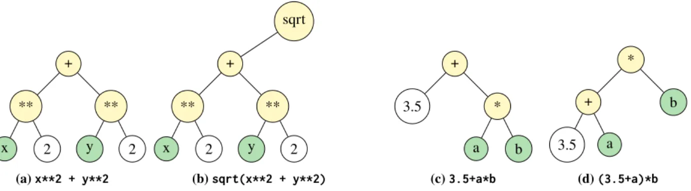
conditionchild of each node, and by treating specific floating point values as booleans (1.0 = True, 0.0 = False, for instance). Fig. 10 depicts a few sample binary syntax trees. Note that the parsing algorithm must observe both the precedence rules and associativity of operators. All nodes in the tree are binary. In the case of unary functions, such as
sqrt, the “right” child is an unassociated pointer. With the polymorphism supported by modern Fortran, the four types of node can each be a subclass derived from the base class,cpNode(shown in Fig. 11).
2. The Parsing Algorithm
The parsing algorithm is the most complex portion of the overall calculation expression capability. The algorithm must account for nested calculations embedded in parentheses, operator precedence and associativity, as well as some “corner cases” such as unary negation and redundant parentheses. In general, the calculation parsing algorithm involves
the following steps:
1) If the string begins with “(” and ends with “)”, strip them and recursively call the parsing algorithm on the remaining string.
1m od u l e toposort_module
2i m p l i c i t none
3p r i v a t e
4
5type :: vertex
6!! a vertex of a directed acyclic graph (DAG) 7 integer,d i m e n s i o n(:) ,a l l o c a t a b l e :: edges
8 i n t e g e r :: ivertex = 0 ! vertex number
9 l o g i c a l :: checking = .false.
10 l o g i c a l :: marked = .false.
11 c o n t a i n s
12 p r o c e d u r e :: set_edges
13 end type vertex
14
15 type,p u b l i c :: dag
16 !! a directed acyclic graph (DAG)
17 type( vertex ),d i m e n s i o n(:) ,a l l o c a t a b l e :: vertices
18 c o n t a i n s
19 p r o c e d u r e :: set_vertices => dag_set_vertices
20 p r o c e d u r e :: set_edges => dag_set_edges
21 p r o c e d u r e :: toposort => dag_toposort
22 end type dag
23
24 c o n t a i n s
25
26 s u b r o u t i n e set_edges (me , edges )
27 !! specify the edge indices for this vertex 28 class( vertex ),i n t e n t(inout) :: me
29 integer,d i m e n s i o n(:) ,i n t e n t(in) :: edges
30 a l l o c a t e(me% edges (size( edges )))
31 me% edges = edges 32 end s u b r o u t i n e set_edges
33
34 s u b r o u t i n e dag_set_vertices (me , nvertices )
35 !! set the number of vertices in the dag 36 class(dag),i nt e n t(inout) :: me
37 integer,i nt e n t(in) :: nvertices !! number of vertices
38 i n t e g e r :: i
39 a l l o c a t e(me% vertices ( nvertices ))
40 me% vertices % ivertex = [(i,i=1, nvertices )] 41 end s u b r o u t i n e dag_set_vertices
42
43 s u b r o u t i n e dag_set_edges (me ,ivertex , edges )
44 !! set the edges for a vertex in a dag 45 class(dag),i nt e n t(inout) :: me
46 integer,i n t e n t(in) :: ivertex !! vertex number
47 integer,d i m e n s i o n(:) ,i n t e n t(in) :: edges
48 call me% vertices ( ivertex )% set_edges ( edges )
49end s u b r o u t i n e dag_set_edges
50
51s u b r o u t i n e dag_toposort (me , order )
52!! main toposort routine
53 class(dag),i n t e n t(inout) :: me
54 integer,d i m e n s i o n(:) ,a ll oca ta ble,i n te n t(out) ::
order
55 i n t e g e r :: i,n, iorder
56 n = size(me% vertices )
57 a l l o c a t e( order (n))
58 iorder = 0 ! index in order array 59 do i=1,n
60 if (.not. me% vertices (i)% marked ) &
61 call dfs(me% vertices (i))
62 end do
63
64 c o n t a i n s
65
66 r e c u r s i v e s u b r o u t i n e dfs(v)
67 !! depth - first graph traversal 68 type( vertex ),i n te n t(inout) :: v
69 i n t e g e r :: j
70 if (v% checking ) then
71 error stop 'Error : circular dependency .'
72 else
73 if (.not. v% marked ) then
74 v% checking = .true.
75 if (a l l o c a t e d(v% edges )) then
76 do j=1,size(v% edges )
77 call dfs(me% vertices (v% edges (j)))
78 end do
79 end if
80 v% checking = .false.
81 v% marked = .true.
82 iorder = iorder + 1 83 order ( iorder ) = v% ivertex 84 end if 85 end if 86 end s u b r o u t i n e dfs 87 88end s u b r o u t i n e dag_toposort 89 90end m o d u le toposort_module
Fig. 8 Topological Sorting Module. This code can be used to determine the order in which to serially propagate
a set of segments whose dependencies are specified. The main routine isdag_toposort(), which contains an
internal recursive procedure that performs a depth-first traversal of the graph.
1p r o g r a m main 2use toposort_module 3i m p l i c i t none 4type(dag) :: d 5integer,d i m e n s i o n(:) ,a l l o c a t a b l e :: order 6call d% set_vertices (5)
7call d% set_edges (2 ,[1]) !2 depends on 1
8call d% set_edges (3 ,[5 ,1]) !3 depends on 5 and 1
9call d% set_edges (4 ,[5]) !4 depends on 5
10call d% set_edges (5 ,[2]) !5 depends on 2
11call d% toposort ( order )
12write(* ,*) order ! prints 1,2,5,3,4
13end p r o g r a m main
(a) Topological Sorting Example. The module from Fig. 8 is used to compute the propagation order of a list of segments (in this case represented as integers) whose dependencies are known in advance. S1 S2 S3 S5 S4
(b) DAG Diagram for Segment Dependencies. Here, S2→S1 indicates that segment 2 depends on segment 1 (i.e., segment 2 is inheriting some data from segment 1).
+ ** x 2 ** y 2 (a)x**2 + y**2 sqrt + ** x 2 ** y 2 (b)sqrt(x**2 + y**2) + 3.5 * a b (c)3.5+a*b * + 3.5 a b (d)(3.5+a)*b
Fig. 10 Binary Syntax Trees Associated with Various Infix Expressions.
1type, p u b l i c :: cpnode
2 !! represents a single cpnode of a binary
calculator tree .
3 !! in general type ( cpnode ) variables should always
be pointers .
4 i n t e g e r :: id = 0
5 !! id tag for this cpnode , used for debugging 6 class( cpnode ), p o i n t e r :: left
7 !! pointer to the left child cpnode 8 class( cpnode ), p o i n t e r :: right
9 !! pointer to the right child cpnode 10 class( cpnode ), p o i n t e r :: parent
11 !! points to the parent cpnode ( null for root) 12 c o n t a i n s
13 p r o c e d u r e :: eval => eval_node
14 !! returns the scalar floating point value for
this node.
15 p r o c e d u r e :: set_left => set_left
16 !! sets the left child node 17 p r o c e d u r e :: set_right => set_right
18 !! sets the right child node
19 p r o c e d u r e :: set_parent => set_parent
20 !! sets the parent node
21 p r o c e d u r e :: print => print_node
22 !! set the print bound method for debugging 23 end type cpnode
24
25 type, public, e x t e n d s( cpnode ) :: literal_node
26 !! implementation of cpnode that represents
literal numeric values
27 real(wp) :: value = 0.0 _wp
28 !! the value represented by this node 29 c o n t a i n s
30 procedure, p u bl i c :: eval => eval_literal_node
31 !! evaluation bound method specific to literal
nodes
32end type literal_node
33
34type, public, e x t e n d s( cpnode ) :: variable_node
35 !! implementation of cpnode that represents a
variable value
36 i n t e g e r :: varindex = 0
37 !! index in the array of variable values for this
node
38c o n t a i n s
39 procedure, p u bl i c :: eval => eval_variable_node
40 !! evaluation bound procedure specific to variable
nodes
41end type variable_node
42
43type, public, e x t e n d s( cpnode ) :: func_node
44 !! implementation of cpnode that represents a
function or operator
45 c h a r a c t e r(len= op_len ) :: func = r ep e a t(' ',op_len )
46 !! function or operator name for this node 47 p r o c e d u r e( cpFunc ), nopass , p o i n t e r :: f
48 !! the function represented by this node 49c o n t a i n s
50 procedure, p u bl i c :: set_function
51 !! bound procedure to set the function represented
by this node
52 procedure, p u bl i c :: eval => eval_func_node
53 !! evaluation bound procedure specific to function
nodes
54end type func_node
Fig. 11 Base Class and Derived Classes of Nodes for a Binary Syntax Tree.
• Proceed through the string, keeping track of parentheses “depth”. • If an operator is found and the parentheses depth is zero, store it.
• If we find an operator with lower precedence, it becomes the “splitting operator”
• If the operator found has the same precedence as the current splitting operator but it associates left-to-right, override the current splitting operator.
• If a splitting operator is found then return the following: the operator, the portion of the string left of the operator, and the portion of the string right of the operator.
3) Ifsplit_equation()returns a splitting operator, then
• Form a newFunctionNodeassociated with the splitting operator • Recursively callparse_calc()on the left and right substrings.
– The nodes associated with the left and right substrings become the left and right children of the
FunctionNode.
4) Ifsplit_equation()finds no splitting operator, then test for one of the following conditions:
• Attempt to read the contents of the calculator string into a floating point variable. If no error is raised, the text represents a literal numeric value andparse_calc()returns aLiteralNodeobject.
• Attempt to match the text to the known function names. If it matches, return aFunctionNodeassociated with the function and recursively callparse_calc()on the arguments to the function, setting them to the left and right children of theFunctionNode.
• Attempt to match the text to the known variable names. If it matches,parse_calc()returns aVariableNode
object.
3. Evaluation of Syntax Trees
Once an expression has been parsed and stored as a tree structure, it can be evaluated with a relatively simple algorithm. The polymorphism available in modern Fortran simplifies the logic by allowing evaluation functions that are specific to each class of node:
• Nodes that represent literal numeric values simply return the floating point value which they represent. • Nodes that represent variables,VariableNodes, return the floating point value of their associated variable. • Nodes that represent functions or operators first evaluate their child nodes and then pass those return values as
arguments to the function with which they are associated.
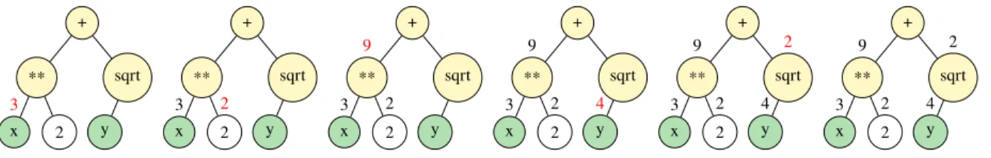
The evaluation algorithm is a recursive, depth-first traversal of the tree in pre-order. If a given node has child nodes, they are evaluated first before evaluating the node itself. Figure 12 demonstrates the evaluation algorithm on a sample tree. + ** x 3 2 sqrt y + ** x 3 2 2 sqrt y + ** 9 x 3 2 2 sqrt y + ** 9 x 3 2 2 sqrt y 4 + ** 9 x 3 2 2 sqrt 2 y 4 + 11 ** 9 x 3 2 2 sqrt 2 y 4
Fig. 12 Example of a recursive evaluation of a tree for the expression"x**2 + sqrt(y)"where x =3and
y=4.
F. Gravity Models
Often, a significant computational component of a high-fidelity spacecraft simulation is the evaluation of the spherical harmonic gravitational field. In Copernicus, the nonsingular algorithm of Pines is used [25], which has been refined by various others over the years [26]. The original published Fortran 77 code [27] is fairly straightforward and does not require much effort to modernize (see, for example, thegeopotential_modulein the Fortran Astrodynamics Toolkit). For small, irregularly-shaped bodies such as asteroids, a polyhedral gravity model may also be used, where the accelerationais computed by the following equation (see Reference [28] for details):
a=∇U=Gσ© « Õ f ∈faces Ff ·rf ·ωf − Õ e∈edges Ee·re·Leª® ¬ (1)
For a very complex polyhedron with many faces, computation of the acceleration is very computationally intensive, but fortunately, the sums are easily parallelizable with OpenMP [29] as shown in Fig. 14, where Eq. (1) is evaluated in a set of two loops (one for the edge terms and another for the face terms).
In Copernicus, the various types of central-body gravity models are extensions of an abstractgravity_model class, part of a general force model for trajectory segments (which can include other gravitating bodies, solar radiation pressure, and atmospheric drag) when they are propagated. Fig. 13 shows the basic concept, where the polyhedral model is an extension of the abstract type, and contains the acceleration routine (get_acc_polyhedral()) shown in Fig. 14). Thepolyhedral_modelclass also contains all the various variables and methods required to compute the acceleration.
1type,abstract,p u b l i c :: gravity_model
2 !! The base abstract class for the various models 3 c o n t a i n s
4 ! each has to define this method :
5 p r o c e d u r e( acc_function ),deferred,p ub l i c :: get_acc
6end type gravity_model
7
8type,e x t e n d s( gravity_model ),p u b l i c :: polyhedral_model
9 !! Polyhedral gravity model 10 c o n t a i n s
11 procedure,p u b l i c :: get_acc => get_acc_polyhedral
12end type polyhedral_model
13
14a b s t r a c t i n t e r f a c e
15 s u b r o u t i n e acc_function (me ,r,a)
16 i m p o r t :: wp , gravity_model
17 class( gravity_model ),i n t e n t(inout) :: me
18 real(wp),d i m e n s i o n(3) ,i n t e n t(in) :: r
19 real(wp),d i m e n s i o n(3) ,i n t e n t(out) :: a
20 end s u b r o u t i n e acc_function
21end i n t e r f a c e
(a) Abstract Gravity Model and Extension.
Gravity Model
Pointmass Polyhedral Geopotential
Pines
(b) General Gravity Model Class Hierarchy
Fig. 13 Thepolyhedral_modelis an extension of the abstractgravity_modelclass. The extended class also
includes an initialization method, and any other methods and data that are needed for the model (not shown here). It inherits all the data and other methods in the base class. For example, while the pointmass model only
contains the gravitational parameter µ, the polyhedral model contains the polyhedral mesh coordinates and
other ancillary data.
G. ODE IVP Solvers
Copernicus includes a large collection of numerical methods for segment propagation, from fixed-step Runge-Kutta and Nyström methods of various orders, to variable-step variable-order Adams methods. There are numerous publicly-available Fortran 77 variable-step variable-order Adams-type codes that work well for the orbit problem (e.g., DLSODE [30], DVODE [31], DDEABM [32], and DIVA‡‡). Very few of these have been updated by the original authors in
decades (CVODE, the C++ successor to DVODE, continues to be developed at LLNL). However, many of the original Fortran 77 codes are fairly easy to improve using modern Fortran concepts. Copernicus includes modernized versions of some of these codes. An open source modernized update to DDEABM is also available§§, which includes new features not available in the original version made possible by the modern language features. The refactored version is object-oriented and thread safe. It also includes a new event finding capability (which incorporates the well-known ZEROIN algorithm for finding a root on a bracketed interval [33]), and the ability to export intermediate points via a user-defined method. Use of the algorithm is via a single class, which can be extended to include the data to be passed into the derivative function.
H. Ephemeris
A celestial body ephemeris is another necessary component of a spacecraft trajectory design and optimization program. Copernicus uses the ephemeris system provided by the Fortran 77 SPICELIB from JPL/NAIF [34], but also allows for pre-splining the ephemeris using various order interpolating B-Splines¶¶. This technique eliminates the
SPICELIB overhead and can result in much faster execution time [35], and also provides a workaround for the fact that SPICELIB is not thread safe. Unfortunately, many classic Fortran codes such as SPICELIB have never moved beyond Fortran 77 and contain all the limitations of a programming language that was superseded almost thirty years ago. SPICELIB is severely restricted by the constraints of Fortran 77 (e.g., maximum number of kernels that can be loaded, maximum number of pool variables, lack of thread safety, impossible to have more than one SPICELIB instance at a time, and a coding style that usesENTRYstatements that were made obsolete by modules in Fortran 90). This is unfortunate since SPICELIB is exceptionally well-written and well-documented code. A modern object-oriented and thread safe SPICELIB could be produced by refactoring the code using modern Fortran techniques, and C-interoperability could be
‡‡JPL MATH77 Library.http://netlib.org/math/
§§Modern Fortran implementation of the DDEABM Adams-Bashforth algorithm.https://github.com/jacobwilliams/ddeabm ¶¶Multidimensional B-Spline Interpolation of Data on a Regular Grid.https://github.com/jacobwilliams/bspline-fortran
1pure s u b r o u t i n e get_acc_polyhedral (me ,r,a)
2
3use iso_fortran_env , only: wp => real64 ! using double precision reals
4
5i m p l i c i t none
6
7class( polyhedral_model ),i n t e n t(in) :: me
8real(wp),d i m e n s i o n(3) ,i nt e n t(in) :: r !! Spacecraft position vector (in body - fixed model frame ) [km]
9real(wp),d i m e n s i o n(3) ,i nt e n t(out) :: a !! Acceleration vector in body - fixed model frame [\( km/s^2 \)]
10
11 real(wp),d i m e n s i o n(3) :: a_sumedge , a_sumface
12 real(wp),d i m e n s i o n(3) :: r1vec ,r2vec , r3vec
13 real(wp),d i m e n s i o n(3) :: temp_vec
14 real(wp) :: l_e ,r1mag ,r2mag ,r3mag ,wf ,numer ,denom ,term
15 i n t e g e r :: i
16
17 a_sumedge = 0.0 _wp; a_sumface = 0.0 _wp ! initialize 18
19 !$omp parallel do default(shared) private(i,r1vec,r2vec,r1mag,r2mag,numer,denom,term,l_e) reduction(+:a_sumedge) 20 do i = 1, me% n_edges ! Edge loop
21
22 r1vec = me%v(:,me% edges (1,i)) - r ! vectors from the field point to the edge endpoints 23 r2vec = me%v(:,me% edges (2,i)) - r
24 r1mag = norm2( r1vec )
25 r2mag = norm2( r2vec )
26 term = r1mag + r2mag ! calculate the logarithm expression , l_e 27 numer = term + me%en(i)
28 denom = term - me%en(i) 29 l_e = log( numer / denom )
30
31 !sum the edge contributions :
32 a_sumedge = a_sumedge + m at m u l(me%ee(i)% matrix *l_e , r1vec ) ! acceleration
33 34 end do
35 !$omp end parallel do 36
37 !$omp parallel do default(shared) private(i,r1vec,r2vec,r3vec,r1mag,r2mag,r3mag,numer,denom,term,wf,temp_vec) reduction(+:a_sumface) 38 do i = 1, me% n_plates ! Face loop
39
40 r1vec = me%v(:,me%p(1,i)) - r ! vectors from field point to face vertices 41 r2vec = me%v(:,me%p(2,i)) - r
42 r3vec = me%v(:,me%p(3,i)) - r 43 r1mag = norm2( r1vec )
44 r2mag = norm2( r2vec )
45 r3mag = norm2( r3vec )
46 numer = d o t _ p r o d u c t(r1vec , cross (r2vec , r3vec ))
47 denom = r1mag * r2mag * r3mag + &
48 r1mag *d o t _ p r o d u c t(r2vec , r3vec ) + &
49 r2mag *d o t _ p r o d u c t(r3vec , r1vec ) + &
50 r3mag *d o t _ p r o d u c t(r1vec , r2vec )
51 wf = 2.0 _wp * atan2( numer , denom ) ! calculate the solid angle term , wf
52
53 !sum the face contributions
54 temp_vec = m a tm u l(me%ff(i)% matrix *wf , r1vec )
55 a_sumface = a_sumface + temp_vec ! acceleration 56
57 end do
58 !$omp end parallel do 59
60 a = me% gdensity *( a_sumface - a_sumedge ) ! acceleration (see Equation 1) 61
62 end s u b r o u t i n e get_acc_polyhedral
Fig. 14 Polyhedral Gravity Acceleration Core Routine. This is a method in thepolyhedral_modelclass (an
extension of the abstractgravity_modelclass shown in Fig. 13). The class contains all the necessary data such as the vertex coordinates (me%v), plate indices (me%p), edge indices (me%edges), edge lengths (me%en), edge matrices (me%ee), and the face normal outer products (me%ff). All of these quantities are computed when the class is initialized. See [29] for a detailed description of this code.
1s u b r o u t i n e ballistic_derivs (me ,et ,x, xdot )
2
3class( segment ),i n t e n t(inout) :: me
4real(wp),i n t e n t(in) :: et !! ephemeris time [sec]
5real(wp),d i m e n s i o n(:) ,i nt e n t(in) :: x !! state [r,v] in inertial frame (moon - centered )
6real(wp),d i m e n s i o n(:) ,i nt e n t(out) :: xdot !! derivative of state [dx/dt]
7
8reaL(wp),d i m e n s i o n(6) :: rv_earth_wrt_moon , rv_sun_wrt_moon
9real(wp),d i m e n s i o n(3 ,3) :: rotmat
10 real(wp),d i m e n s i o n(3) :: r,rb ,v, a_geopot ,a_earth , a_sun
11 l o g i c a l :: status_ok
12
13 r = x (1:3) ; v = x (4:6) ! get state
14 rotmat = icrf_to_iau_moon (et) ! rotation matrix from inertial to body - fixed Moon frame 15 rb = m a t m u l(rotmat ,r) ! r in body - fixed frame
16
17 call me% grav % get_acc (rb , a_geopot ) ! get the acc due to the geopotential
18 a_geopot = m a t m u l(t r a n s p o s e( rotmat ),a_geopot ) ! convert acc back to inertial frame
19
20 call me%eph% get_rv (et , body_earth , body_moon , rv_earth_wrt_moon , status_ok ) ! 3rd body vecs ( inertial wrt moon)
21 call me%eph% get_rv (et , body_sun , body_moon , rv_sun_wrt_moon , status_ok )
22
23 a_earth = third_body_gravity (r, rv_earth_wrt_moon (1:3) ,mu_earth ) ! 3rd body perturbations 24 a_sun = third_body_gravity (r, rv_sun_wrt_moon (1:3) ,mu_sun )
25
26 xdot = [v, a_geopot + a_earth + a_sun ] ! total derivative vector 27
28 end s u b r o u t i n e ballistic_derivs
Fig. 15 Ballistic Equations of Motion for a Spacecraft in the Vicinity of the Moon. In this example Fortran
Astrodynamics Toolkit usage, asegmentclass contains an instance of a ephemeris (eph) as well as a geopotential
gravity model (grav) for the Moon. The ephemeris is used to compute the perturbations from the Earth and
Sun.
used to provide interfaces to other programming languages. Virtually none of the mathematical code would need to be modified. Be that as it may, NAIF has recently announced that a modern edition of SPICELIB will be produced by rewriting the entire library in C++.
A modern Fortran object-oriented celestial body ephemeris system has been created that is based on the legacy Fortran 77 JPLEPH code [36]. This system is included in the Fortran Astrodynamics Toolkit, and is a fairly light refactoring of the original code (as none of the mathematics have changed). The ephemeris is a class, and it allows for thread-safe use and multiple instantiations, neither of which are possible in either the original code or SPICELIB. The ephemeris class can be employed for the trajectory segment propagation problem by having a segment include an instance of an ephemeris. An example use case for this is shown in Fig. 15, where the equations of motion of a spacecraft at the Moon include the third-body perturbations from the Earth and Sun. An ephemeris is also necessary for certain state transformations (for example conversion between an inertial frame and an Earth-Moon rotating frame), so a general-purpose state transformation class also requires an instance of the ephemeris to be input to the transformation method.
I. Optimizers & Nonlinear Equation Solvers
Historically, much of spacecraft trajectory optimization at NASA has been done using Fortran 77 solvers such as VF13AD [37], SLSQP [38], NPSOL, SNOPT [39], and IPOPT [40] (IPOPT originally was written in Fortran, and though eventually converted to C++, still includes many third-party Fortran components). These general solvers can be used to solve nonlinear programming problems to minimize a scalar objective function subject to general equality and inequality constraints and to lower and upper bounds on the variables. Most complex problems in Copernicus are solved using SNOPT, which has proven very effective for very large and sparse trajectory problems. A new modern Fortran version of SNOPT has been under development for some time. SLSQP (suitable only for smaller problems) is also available in Copernicus and OTIS (as well as the Python SciPy package), and a new open source modern Fortran refactoring is also available∗∗∗.
For some problems not requiring optimization, a very simple differential corrector solver can often be used [41].
1s u b r o u t i n e nle_solver (me ,x)
2
3class( nle_solver_class ),i n t e n t(inout) :: me
4real(wp),d i m e n s i o n(:) ,i nt e n t(inout) :: x !! control variable vector
5
6i n t e g e r :: iter
7real(wp),d i m e n s i o n(me%m,me%n) :: fjac !! jacobian matrix
8real(wp),d i m e n s i o n(me%n) :: p !! search direction
9real(wp),d i m e n s i o n(me%m) :: fvec !! function vector
10
11 fvec = me% func (x) ! evaluate the function at the initial point 12 do iter = 1,me% max_iter
13 fjac = me% grad (x) ! compute the jacobian matrix
14 p = linear_solver (fjac ,- fvec ) ! compute the search direction p by solving linear system
15 ! [ this is just a wrapper for DGELS ]
16 x = x + me% alpha * p ! compute new x
17 fvec = me% func (x) ! evaluate the function at the new point 18 if (m a x v a l(abs( fvec )) <= me% ftol ) exit ! check for convergence in f
19 end do
20
21 end s u b r o u t i n e nle_solver
Fig. 16 Overview of a Differential Corrector Solver. Thefunc()andgrad()functions in thenle_solver_class
are user-supplied functions defined when the base class is extended (all the data necessary to compute the functions is contained in the class, thus the solver code can be very generic).
Solvers of this sort use a Newton-style iteration step from a previous control vectorxk to the next onexk+1, using:
xk+1=xk−αJ−1f(xk) (2)
wherexis then×1 vector of control variables,fis them×1 vector of constraint violations, andJis them×nJacobian matrix. Ifn>mthenJ−1is the minimum norm pseudoinverse of the underdetermined linear system, which can be computed, for example, using the LAPACKdgels()subroutine. See Fig. 16 for a very basic overview of this type of code. A robust, general purpose solver is much more complex than the example shown here, and includes error checking, other types of convergence and singularity checks, as well as various options for computing the step sizeα (for example, by using a line search). For square systems (n×n) there are many publicly available high-quality Fortran 77 solvers, such as HYBRJ from MINPACK, an implementation of the Powell hybrid method [42].
J. Gradients
Gradient-based solvers and optimizers (such as SNOPT) require computation of the derivatives of the objective function and the constraints with respect to the control variables (i.e., the Jacobian). Some solvers (such as IPOPT) also allow or require the input of second derivative information as well (i.e., the Hessian). Computing the gradients can be the most time-consuming part of the optimization problem, and accurate gradients are critical to successful convergence.
The classical method to compute gradients is via finite differences. Finite differences have the advantage of being simple to compute, and they can be used if the function contains third-party or “black-box” components. Copernicus primarily uses finite differences to compute gradients (although other methods are also available such as differentiation of interpolating polynomials such as cubic splines). Iffn = f(x+nh)is a function evaluation given a control variablexand
a perturbationh, then the set of three-point finite differences approximating the derivative atxare(−3f0+4f1−f2)/(2h), (−f−1+f1)/(2h), and(f−2−4f−1+3f0)/(2h). In practice, the second one (the classical central difference method)
is often used, but the others are useful if the central difference would violate the variable bounds (for example, if the function is undefined beyond a certain bound). Copernicus includes a full set of formulas from two to eight points [43], as well as algorithms for tuning the step sizeh(which is critical when using finite differences) [44]. A new open source object-oriented finite-difference library (NumDiff) is also available with a variety of user-selectable methods††† including from two to six point formulas as well as Neville’s algorithm [45]. NumDiff also includes an implementation of a graph coloring algorithm for efficient computation of the Jacobian by taking advantage of the sparsity pattern [46]. Another Fortran numerical differentiation library also exists that employs OpenMP and MPI for parallelization [47].
For applications where the user has full control of the problem function and all the source code, other types of gradient methods are also possible. Since complex numbers are natively supported in Fortran, complex-step differentiation
1m od u l e operator_overloading
2
3use iso_fortran_env , only: wp => real64
4i m p l i c i t none 5 6p r i v a t e 7 8type,p u b l i c :: a_real 9 p r i v a t e 10 real(wp),p ub l i c :: value = 0.0 _wp 11 real(wp),p ub l i c :: grad = 0.0 _wp
12 end type a_real
13
14 i n t e r f a c e o p e r a t o r(*) ! overload multip . operator
15 m o d u l e p r o c e d u r e :: aa_multiply
16 end i n t e r f a c e
17 p ub l i c :: o p e r a t o r(*)
18
19 i n t e r f a c e sin ! overload sin () function
20 m o d u l e p r o c e d u r e :: a_sin 21 end i n t e r f a c e 22 p ub l i c :: sin 23 24 c o n t a i n s 25
26 pure e l e m e n t a l f u n c t i o n aa_multiply (a,b) r e s u l t(c)
27 !! a_real * a_real
28 type( a_real ),i n t e n t(in) :: a
29 type( a_real ),i n t e n t(in) :: b
30 type( a_real ) :: c
31 c = a_real (a% value * b%value ,&
32 b% value *a%grad + a% value *b%grad) 33end f u n c t i o n aa_multiply
34
35pure e l e m e n t a l f u n c t i o n a_sin (a) r e s u l t(c)
36 !! sin( a_real )
37 type( a_real ),i n t e n t(in) :: a
38 type( a_real ) :: c
39 c = a_real (sin(a% value ), cos(a% value )*a%grad)
40end f u n c t i o n a_sin 41 42end m o d u l e operator_overloading 43 44p r o g r a m operator_overloading_test 45
46use iso_fortran_env , only: wp => real64
47use operator_overloading 48 49i m p l i c i t none 50 51type( a_real ) :: x,z 52
53x = a_real (2.0 _wp ,1.0 _wp) ! get derivative w.r.t. x 54z = x*sin(x) ! computes value and dz/dx
55
56write(* ,*) z%value , z%grad ! 1.818594 , 0.077003
57
58end p r o g r a m operator_overloading_test
Fig. 17 Operator Overloading to Compute Gradients. In this example, we define a newa_realtype to replace
allrealvariables in a set of calculations where gradients are required. For the most general case, all operators, assignments, and intrinsic functions must be overloaded. In this example, it is shown how to overload the multiplication operator and thesin()function to compute the function value (z) and gradient (dz/dx) for the functionz(x)=xsinxwhenx=2.
is an option [48]. Operator overloading (see Fig. 17 for a basic example) can also be used to compute the gradients analytically. Various modern Fortran libraries are available for differentiation using operator overloading‡‡‡ [49]. Finally, quadruple precision (real128, which is natively supported in Fortran), or even arbitrary precision (available via third-party libraries [50]) can be employed to reduce roundoff error in computations and produce more accurate finite difference gradients.
III. Coarray Fortran
Thanks to the introduction of coarrays, Fortran is a partitioned global address space (PGAS) language, allowing programmers to write parallel programs in standard conforming Fortran without relying on third party libraries or compiler directives and extensions. Coarray Fortran (CAF) [51, 52] has been part of the Fortran language since the 2008 standard.
A defining characteristic of PGAS languages is the ability to perform operations withglobalmemory, regardless of whether the machine is a leadership-class, petascale HPC cluster, or a shared-memory laptop. This presents the application programmer with a consistent programming model across different computer architectures, including distributed memory, shared memory, and heterogeneous systems. Another feature of PGAS languages is the ability to manipulate remote memory through fetching remote values, “gets,” or storing remote values, “puts,” without directly involving the processing element (PE) that “owns” the memory in question. This presents the programmer with a simplified programming model reminiscent of shared memory paradigms, even when the program is running across many nodes of a distributed and/or heterogeneous system. In PGAS languages the burden of explicitly coordinating communication between the sender(s) and receiver(s) is removed; one-sided communication is the default, and less time is spent waiting and coordinating with remote PEs relative to the more common two sided message passing paradigms. A one-sided communication strategy is achievable with the Message Passing Interface (MPI), as of MPI-3, but only at the cost of substantial additional complexity and programmer effort. An advantage of one-sided communication is that whenever hardware support for remote direct memory access (RDMA) is present, the remote PE need not be involved in the data transfer at all, both at the program and operating system (OS) level [53]. Computations on the remote image
may proceed uninterrupted while data is delivered or retrieved, thus overlapping communication with computation. While all PGAS languages present some access to global memory, they may differ in other, substantial ways. Some PGAS languages, such as Chapel [54] do their best to provide high-level interfaces that can hide and abstract all details about parallelism from the application programmer. While Chapel does provide a means to take more explicit control of the parallelism when required, many programs can be written in such a way that they appear no different than serial programs. Other PGAS languages, or language extensions such as XcalableMP [55], provide “global view” objects where the array objects appear to be indexed conventionally, but ranges of indices reside on physically distinct distributed memories. For example, a “global view” matrix is represented as a two-dimensional array with non-overlapping portions residing in physically distinct memories. While such a “global view” object could be emulated with CAF, the CAF programming model is closer to a more traditional single program, multiple data (SPMD) paradigm.
The parallelism in CAF derives from two key concepts:imagesandcoarrays. When a CAF program is launched, it is replicatedNtimes. Each copy is called animageand is approximately analogous to an MPI “rank.” The intrinsic functionthis_image()returns the image index of the current image, allowing each image to distinguish itself, and the intrinsic functionnum_images()provides access to the total number of images,N, spawned. Each variable is local to the image, and cannot be accessed by remote images unless it is declared as a coarray. Arrays and scalars, both statically and dynamically allocated, of intrinsic or user defined type, may be declared as coarrays, with some restrictions. Coarrays differ from other variables in that they are declared with a codimension having cobounds. The codimension utilizes square brackets to distinguish it from traditional array dimensions denoted by parentheses (see Fig. 18). The number of images spawned is fixed before the program is launched, usually specified by an environment variable or a job launcher script on distributed memory systems. Once the program is launched, the number of images cannot be altered. As a consequence, the last codimension is never explicitly specified in the program and must be syntactically specified with an asterisk when a coarray variable is declared or allocated. Each image in a CAF program corresponds to a single partition of a global address space. Coarray variables are entities in this global address space that can be retrieved or modified from any partition, when a coindex is specified.
Coordination and reasoning about parallel CAF programs is achieved through the concept ofexecution segmentsand
image control statements. Image control statements are either explicit or implicit coordinations and synchronizations between different images. A list of CAF image control statements is given in Table 2. Image control statements separate
execution segments, which are the mechanism that allows reasoning about global program state. If an execution segment
mon imageP(Pm) is terminated by an image control statement that matches a corresponding image control statement
demarcating the beginning of an execution segmentnon imageQ(Qn) then execution segmentPmis said to be ordered
with respect toQnand to precede it. In such a case, a “get,” performed in segmentQnof a coarray variable residing
on imagePand modified in execution segmentPmyields the expected value. Similarly a “put” of a coarray variable
where segmentQnwrites to a variable residing on imagePensures that the write happens after segmentPmis finished
executing. If images areun-orderedwith respect to each-other, then the behavior of “gets” and “puts” is undefined if the coarray variable in question is also locally modified or used. In un-ordered segments there is no guarantee that a “get” of a coarray variable that is locally modified during the un-ordered segments will yield the value before or after the modification, and, similarly, a “put” of a coarray variable read locally in the segments may or may not overwrite the variable before, after, or while it is being read. Ordered segments provide a means to guarantee the state of remote coarray variables. A few lines of source code demonstrating these principles is shown in Fig. 18.
The chief benefits of choosing CAF over other parallel runtime solutions are that CAF provides a small but powerful and flexible API that is easy to learn, is architecture and implementation agnostic, and is portable and performant. The programmer is not tied to any particular architecture (shared vs. distributed memory) or implementation technology. As technologies change, the same CAF program can be run on new systems, using new network fabrics or back end transport layers without any modification required by the programmer. With a suitable implementation, such as GFortran with OpenCoarrays,§§§[56] it may even be possible to switch the underlying communication technology by simply re-linking the program [57]. This is useful if a bug or defect is discovered in an underlying component. CAF has a much more concise API than many other alternatives like MPI, which has hundreds of procedure calls to learn. Therefore, learning CAF is less of a burden on programmers, and enables performant one-sided communication characteristic of PGAS languages. The one-sided nature allows programmers to overlap communication and computation, thus hiding the latency associated with communication. Compilers are free to make arbitrary optimizations including out of order execution and code movement within an execution statement, so a smart enough compiler can perform some optimizations on both “puts” where the coindex appears on the left hand side of an assignment, as well as “gets” where