els for imputing missing data using MICE: a CALIBER study. Amer-ican journal of epidemiology, 179 (6). pp. 764-74. ISSN 0002-9262 DOI: https://doi.org/10.1093/aje/kwt312
Downloaded from: http://researchonline.lshtm.ac.uk/1883884/ DOI:10.1093/aje/kwt312
Usage Guidelines
Please refer to usage guidelines at http://researchonline.lshtm.ac.uk/policies.html or alterna-tively [email protected].
Available under license: Creative Commons Attribution Non-commercial http://creativecommons.org/licenses/by-nc/3.0/
Practice of Epidemiology
Comparison of Random Forest and Parametric Imputation Models for Imputing
Missing Data Using MICE: A CALIBER Study
Anoop D. Shah*, Jonathan W. Bartlett, James Carpenter, Owen Nicholas, and Harry Hemingway
*Correspondence to Dr. Anoop D. Shah, Clinical Epidemiology Group, Department of Epidemiology and Public Health, School of Life and Medical Sciences, University College London, Wolfson House, 2-10 Stephenson Way, London NW1 2HE, United Kingdom (e-mail: [email protected]). Initially submitted April 5, 2013; accepted for publication November 20, 2013.
Multivariate imputation by chained equations (MICE) is commonly used for imputing missing data in epidemio-logic research. The“true”imputation model may contain nonlinearities which are not included in default imputation models. Random forest imputation is a machine learning technique which can accommodate nonlinearities and in-teractions and does not require a particular regression model to be specified. We compared parametric MICE with a random forest-based MICE algorithm in 2 simulation studies. The first study used 1,000 random samples of 2,000 persons drawn from the 10,128 stable angina patients in the CALIBER database (Cardiovascular Disease Re-search using Linked Bespoke Studies and Electronic Records; 2001–2010) with complete data on all covariates. Variables were artificially made“missing at random,”and the bias and efficiency of parameter estimates obtained using different imputation methods were compared. Both MICE methods produced unbiased estimates of (log) haz-ard ratios, but random forest was more efficient and produced narrower confidence intervals. The second study used simulated data in which the partially observed variable depended on the fully observed variables in a nonlinear way. Parameter estimates were less biased using random forest MICE, and confidence interval coverage was bet-ter. This suggests that random forest imputation may be useful for imputing complex epidemiologic data sets in which some patients have missing data.
angina, stable; imputation; missing data; missingness at random; regression trees; simulation; survival
Abbreviations: CALIBER, Cardiovascular Disease Research using Linked Bespoke Studies and Electronic Records; MAR, missing at random; MICE, multivariate imputation by chained equations.
Missing data are a pervasive problem in epidemiologic studies, particularly for research using routinely collected clinical health records (1). Incomplete data sets are frequently analyzed using multiple imputation, which involves creating multiple complete versions of the data with missing values imputed through random draws from distributions inferred from observed data (2). Multiple imputation typically as-sumes that data are missing at random (MAR)—that is, that missingness is not associated with the missing value, condi-tional on the observed data (3). Multivariate imputation by chained equations (MICE), also called full conditional spec-ification, is a common method of generating imputed values by drawing from estimated conditional distributions of each variable given all the others (4). Imputation models must be appropriately specified for analyses based on imputed data to
yield unbiased parameter estimates and associated standard errors. The default setting in implementations of MICE is for imputation models to include continuous variables as lin-ear terms only with no interactions, but omission of important nonlinear terms may lead to biased results (5). Other potential problems with parametric regression models are that 1) they cannot include more predictor variables than the number of observations without recourse to prior information (6) and 2) inclusion of highly correlated variables may cause prob-lems due to collinearity. In this paper, we propose a new im-putation method which aims to overcome these problems using random forest.
Random forest is an extension of classification and regres-sion trees (7), predictive models that recursively subdivide the data based on values of the predictor variables. They do provided the original work is properly cited. January 12, 2014
not rely on distributional assumptions and can accommodate nonlinear relations and interactions. On simulated data sets with interactions between variables, imputation of missing data using MICE with regression trees resulted in less biased parameter estimates than MICE with linear regression (7). However, regression trees may“overfit,”following the pat-tern of noise too closely and producing a complex model with poor predictive power in new data sets.
Random forest uses bootstrap aggregation of multiple re-gression trees to reduce the risk of overfitting, and it com-bines the predictions from many trees to produce more accurate predictions (8,9). Random forest is widely used in genetic epidemiology (10) and has also been used for mod-eling survival (11,12) and predicting response to cancer che-motherapy (13). We propose that random forest may be useful in multiple imputation of epidemiologic data sets, par-ticularly if there are large numbers of clinical variables per participant, as may increasingly be the case (e.g., genomic or proteomic studies).
Stekhoven et al. (14) developed a random forest-based al-gorithm for missing data imputation called missForest. This algorithm aims to predict individual missing values accurately rather than take random draws from a distribu-tion, so the imputed values may lead to biased parameter es-timates in statistical models. Apart from a comparison between random forest and polytomous regression for imput-ing tumor stage usimput-ing MICE (15), we are not aware of other published evaluations of multiple imputation using random forest.
In this paper, we compare a standard implementation of MICE with imputation using missForest, and we propose a new version of MICE which imputes each variable using ran-dom forest. We compare these methods in a realistically com-plex survival analysis based on patients with stable angina in the CALIBER (Cardiovascular Disease Research using Linked Bespoke Studies and Electronic Records) database (16) and in a simulation study with interactions.
METHODS
Imputation of missing data using MICE, where each variable is imputed using random forest
Within the MICE framework, missing values of continu-ous variables are conventionally imputed byfitting a linear regression model for the observed values, predicting the con-ditional mean for each missing value, and randomly imputing a value from a normal distribution centered on this condi-tional mean. Our new method is derived from the“mice. impute.norm.boot”function in the“mice”package in R (4), in which linear regression is applied to a bootstrap sample of rec-ords with observed values of the variable to be imputed. The purpose of the bootstrap is to accommodate sampling varia-tion in estimating populavaria-tion regression parameters, which is part of ensuring that imputations are“proper”(3). The ran-dom forest algorithm itself involves another level of bootstrap sampling. Records with missing values in the dependent var-iable are imputed by random draws from independent normal distributions centered on conditional means predicted using random forest. We used the“out-of-bag”mean square error
as the estimator of residual variance (which we assumed to be normally distributed). Random forestfits each tree to a dif-ferent bootstrap sample of the data and aggregates the results; the out-of-bag error is the mean of squared differences be-tween each observed value and the prediction based on trees for which that observation is not included in the boot-strap sample.
For binary or unordered categorical variables, we used ran-dom forest tofit individual regression trees to a bootstrap sample of the data and imputed each missing value as the pre-diction of a randomly chosen tree. This is equivalent to choosing between 0 and 1 with probability according to the mean random forest prediction. Our random forest imputation functions are available from the Comprehensive R Archive Network (17).
Simulation study based on CALIBER data
CALIBER is a database of linked routinely collected elec-tronic health records from England (16), comprising data from primary care (Clinical Practice Research Datalink) (18), hospital admissions (19), the national registry of acute coronary syndromes (20), and the national death registry.
The cohort consisted of patients who received a diagnosis of stable angina while registered at a general practice contrib-uting to the Clinical Practice Research Datalink. Blood pres-sure, smoking status, and measurements of blood biomarkers were taken from routine clinical records before the diagnosis of stable angina, and patients were followed up for the com-posite endpoint of death or nonfatal myocardial infarction (see Web Appendix 1, available athttp://aje.oxfordjournals. org/). The CALIBER record-linkage study has received eth-ical approval, and this study was approved by the Clineth-ical Practice Research Datalink Independent Scientific Advisory Committee.
Analysis of interest. We investigated missing data in the context of a hypothetical analysis of associations, suggested in previous studies (21–23), between 3 commonly measured hematological parameters (hemoglobin concentration, lym-phocyte count, and neutrophil count) and prognosis among patients with stable angina in CALIBER. The substantive analysis was a multivariable Cox model with the composite endpoint of death or nonfatal myocardial infarction, and with predictor variables specified a priori.The fully observed predictor variables were: age, age squared, sex, previous myocardial infarction, diabetes mellitus, previous stroke, peripheral arterial disease, and heart failure. Smoking status was a partially observed 3-category variable (never, former, or current smoker), and we included the following partially observed continuous variables: systolic blood pressure (mm Hg), log neutrophil count (109cells/L), log lymphocyte count (109cells/L), high-density lipoprotein cholesterol level (mmol/L), hemoglobin concentration (g/dL), and log serum creatinine concentration (µmol/L). For each of these vari-ables, we took the mean of any observed values in the 2 years prior to the start of follow-up. We used the Efron ap-proximation (24) for ties. We did not investigate alternative models and ignored clustering by general practice.
Generation of sample data sets for simulation study. For the simulation study, we created data sets with missing data
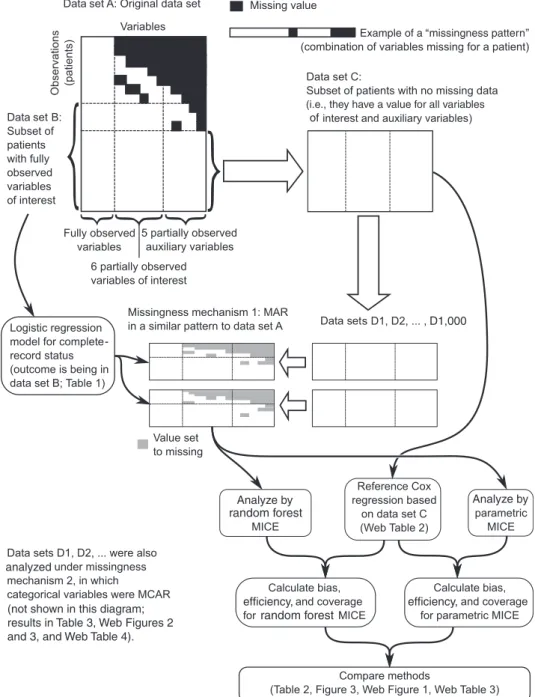
for which we knew the“true”values, with a missingness pat-tern similar to that observed in the actual data set but which was missing at random, such that the MAR assumption un-derlying most multiple imputation approaches was satisfied (Figure1). We denoted the entire cohort of 52,576 stable an-gina patients data set“A.”Patients with no missing values for any of the variables in the survival model were denoted data set“B”(13,308 patients).
We used logistic regression based on completely observed variables to investigate factors associated with a patient’s
having a complete record (i.e., whether a patient was in data set B). We included thefirst value after cohort entry of partially observed continuous variables as auxiliary variables to help predict missing covariates in imputation models. The subset of patients with complete recording of all analysis and auxiliary variables was denoted data set“C” (10,128 pa-tients), and they formed the basis for the resampling study. We artificially made some values of predictor variables miss-ing in one thousand 2,000-patient random samples (with re-placement) from data set C. We carried out simulations with
Figure 1. Generation of data sets with artificial missingness from a population of patients with stable angina in the CALIBER database, 2001– 2010. Data sets D1, D2, . . . , D1,000 are samples of 2,000 patients with replacement from data set C. CALIBER, Cardiovascular Disease Research using Linked Bespoke Studies and Electronic Records; MAR, missing at random; MCAR, missing completely at random; MICE, multivariate impu-tation by chained equations.
one of 2 missingness mechanisms: 1) MAR in a pattern similar to that of data set A or 2) an artificial pattern of missingness completely at random in which only categorical variables were missing (see Web Appendix 1 for more details).
Multiple imputation of test data sets. Imputation models included all of the variables in the substantive Cox model, event status, marginal Nelson-Aalen cumulative hazard (25), and the following auxiliary variables: type of endpoint, whether the practice was receiving electronic laboratory results, and the earliest recorded value after the index date for blood pressure and the 5 blood biomarkers. We imputed continuous variables using MICE with normal-based linear regression, predictive mean matching with 3 nearest neigh-bors, and our new random forest method. We imputed categor-ical variables using either MICE with logistic or polytomous regression or MICE with random forest (choice of 10 or 100 trees). We also investigated random forest with a single tree to determine whether bootstrap aggregation had an advantage over a single regression tree.
We generated 10 MICE imputations, each drawn from a separate chain with a different random seed, with 10 cycles of imputation before drawing the imputed data set. We as-sessed chain mixing by reviewing plots of chain mean values and standard deviations. For two of the methods (random for-est with 10 trees and parametric MICE), we also calculated results using 100 imputations.
In addition to MICE, we also evaluated missForest (14), which uses random forest in an iterative way to complete a data set with missing values, where imputed values are equal to the random forest predictions rather than being ran-domly sampled from a conditional distribution. We generated multiple imputed data sets by running missForest using dif-ferent random seeds, which leads to difdif-ferent random forest models being generated.
Regardless of the imputation method, all data sets were an-alyzed using the same multivariable semiparametric Cox model as described above. For each set of imputed data sets, the log hazard ratios from the Cox model were combined using Rubin’s rules (26), which assumes that imputed values were drawn from the appropriate Bayesian posterior. We car-ried out analyses using R 2.12.1 (27), with the software pack-ages mice 2.12 (4), missForest 1.3 (28), survival 2.36-2 (29), and randomForest 4.6-6 (30). Random numbers were gener-ated using the Mersenne Twister (31).
Comparison of results obtained by different methods. We considered the Cox proportional hazards modelfitted to the entire data set (data set C) the“true”result for the assess-ment of bias and confidence interval coverage of hazard ra-tios. We compared the widths of 95% confidence intervals between 2 methods using paired-samplet tests. We com-pared coverage of 95% confidence intervals for each coeffi -cient separately using McNemar’s test, defining discordant pairs as data sets in which the 95% confidence interval in-cluded the “true”value for one method but not the other. We compared the efficiency of the estimators by calculat-ing their empirical standard deviations. We calculated the between-imputation variance of the estimated log hazard ra-tios, defined as the mean (across simulations) of the variance of the log hazard ratio estimates from the 10 imputations per data set.
Simulation study with interactions
We also created simulated data sets to compare the per-formance of methods when there were nonlinearities in the association between predictor variables. We generated 2 independent random normal variables with mean 0 and variance 1,x1andx2, and a third variablex3equal to 0.5(x1+ x2−x1x2) +e, whereewas distributed normally with mean 0 and variance 1. Survival times were generated according to an exponential distribution with log hazard 0.5(x1+x2+ x3). This meant that there were no interactions in the substan-tive model, but the default parametric imputation model for x3(which would not include any interactions) would be in-correct. Observation times were generated according to a uni-form distribution in the range from 0 to the 50th percentile of survival times. If the observation time was less than the survival time, the patient was considered censored (event indicator 0, and the patient’s follow-up ended on his or her censoring date); otherwise the event indicator was 1, with follow-up ending on the date of the event.
Variablex3was made 20% MAR according to a logistic model based onx1andx2, the marginal Nelson-Aalen cumu-lative hazard and the event indicator.
We analyzed 1,000 simulated data sets with 2,000 patients each, imputing missing data using random forest and para-metric MICE (without interactions), comparing the results as above (Web Appendices 2 and 3).
RESULTS
Simulation study based on CALIBER data
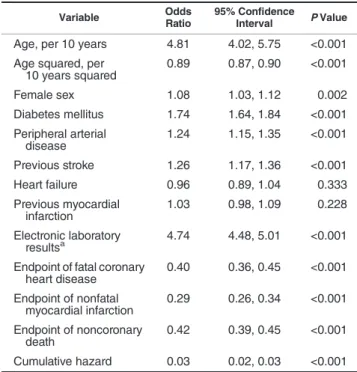
The prevalence of missingness among partially observed variables ranged from 1.5% for smoking to 56.7% for lympho-cyte counts and 56.8% for neutrophil counts (Web Table 1). Patients with missing data were more likely to experience the primary endpoint of death or nonfatal myocardial infarc-tion (age- and sex-adjusted hazard ratio = 1.19, 95% confi -dence interval: 1.13, 1.25) (Figure2). Patients with missing data also tended to have longer follow-up because they entered the cohort earlier (a median index date of March 1, 2002, vs. December 6, 2005;P< 0.0001 by Wilcoxon rank-sum test). The logistic regression model showed that patients with diabe-tes, peripheral arterial disease, and previous stroke were more likely to have complete records (Table1). Web Table 2 shows that coefficients from Cox models for patients with complete data (data set C) were similar to the average results from full data analysis of the subsamples (as we would expect in the ab-sence of small-sample bias), so we compared imputation esti-mates with those from data set C.
We found very little difference between results obtained using 10 MICE imputations and those obtained using 100 MICE imputations (Web Tables 3 and 4), so all results are based on 10 imputations unless stated otherwise.
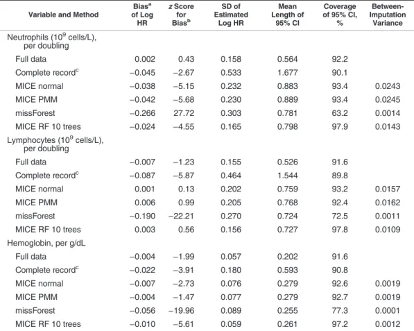
Bias. Estimates from complete-record analysis were biased for some parameters under MAR (missingness mechanism 1); this may be expected because we had intro-duced missingness dependent on the outcome (Table 2, Web Table 3, Web Figure 1). For example, the geometric mean hazard ratio per doubling of lymphocyte count was
0.738 from complete-record analysis but 0.799 from full-data analysis. There was no material bias with parametric MICE (mean hazard ratio = 0.806) or our random forest MICE
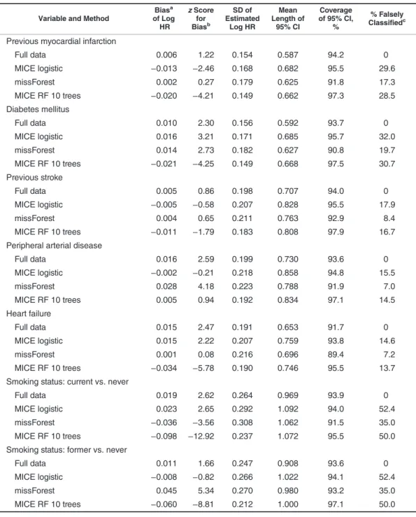
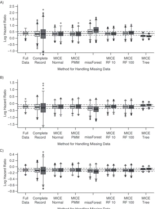
method with 10 trees (“MICE RF 10”; mean hazard ratio = 0.807). The random forest MICE estimate for smoking (cat-egorical) was biased towards the null (Table3, Web Figure 2), but there was no material bias in other parameters estimated by random forest or parametric MICE (Table2, Web Tables 3 and 4, Web Figure 3). However, imputation using single-tree random forest MICE (“MICE Tree”) or missForest produced materially biased estimates for all continuous variables miss-ing at random (Figure3, Table2, Web Figure 1, Web Table 3). Efficiency. All of the imputation methods tested produced more efficient parameter estimates than complete-record anal-ysis. MICE with random forest produced slightly more efficient estimates than parametric MICE, and the average between-imputation variance was also lower (Tables2and3, Web Tables 3–6).
Confidence intervals. Parametric MICE yielded confi -dence intervals with approximately 93%–95% coverage. The mean widths of confidence intervals were lower using random forest MICE than using parametric MICE (P< 0.001 for each comparison), but coverage was either equal or greater using random forest MICE (Tables2and3, Web Tables 3–6).
For categorical variables, missForest produced imputed values which were more likely to be equal to the“true” (ob-served) value than the MICE methods, but confidence inter-vals were too small with below nominal coverage, and between-imputation variance was very small. There was no difference in bias, precision, or coverage between normal-based MICE and predictive mean matching (Web Table 5). Random forest MICE with 100 trees for continuous variables produced estimates with slightly narrower confidence inter-vals than random forest MICE with 10 trees (Web Table 5), but with greater bias, worse coverage of 95% confidence in-tervals, and 10 times the computational cost. For categorical variables, random forest MICE with 10 trees and random for-est MICE with 100 trees produced almost identical results.
Simulation study with interactions
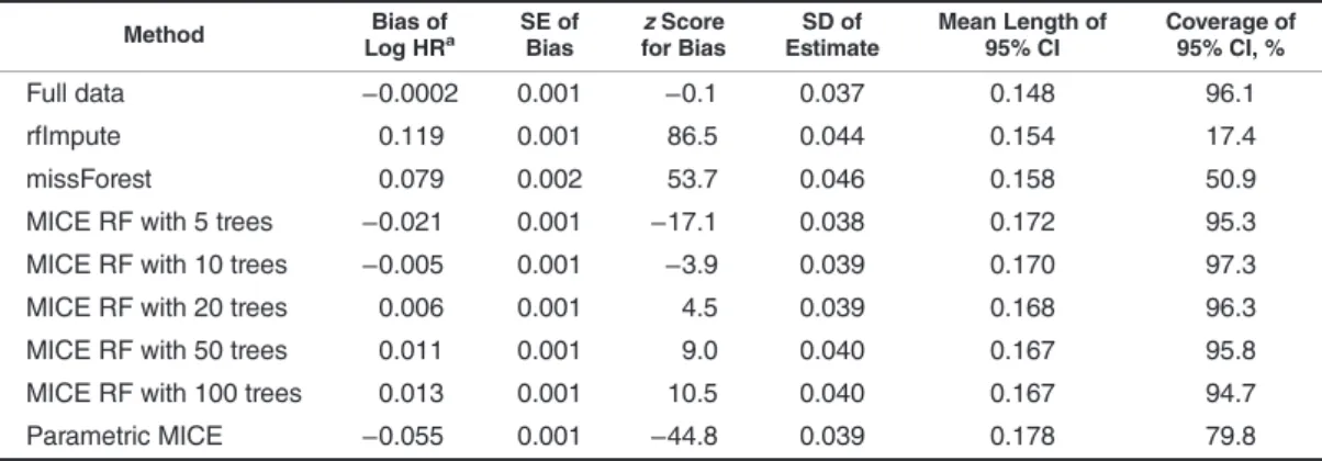
The coefficient estimate for the partially observed variable (x3) was 10% biased using parametric MICE, 2.6% biased using random forest with 100 trees, and only 1.0% biased using random forest with 10 trees (P< 0.001 for 2-way com-parisons). The bias in thex3coefficient varied with the num-ber of trees, with 10 or 20 trees giving minimal bias (Table4). Random forest MICE produced narrower 95% confidence in-tervals for the x3 coefficient than parametric MICE (P< 0.001), and coverage was only 80% using parametric MICE as compared with 95% using random forest MICE with 5– 100 trees. Further details are given in Web Appendix 2.
DISCUSSION
Summary of main findings
In this resampling study of methods for handling missing data, parametric and random forest MICE produced estimates with no material bias for a Cox model on data with artificially introduced MAR missingness. Random forest-based MICE produced more efficient estimates and narrower confidence intervals than parametric MICE, yet in some cases coverage probability was greater than 95%, suggesting that some
Time, years 0 1 2 3 4 5 6 0.1 0.2 0.3 0.4 0
Not data set B Data set B
Figure 2. Cumulative incidence of myocardial infarction or death (Kaplan-Meier failure curve) for patients with stable angina in the CALIBER database, by complete record status, 2001–2010. The solid line represents patients in data set A but not data set B (those with missing data;n= 39,268 at the start, dropping to 17,588 in year 6), and the dashed line represents patients in data set B (those with complete records;n= 13,308 at the start, dropping to 2,594 in year 6). CALIBER, Cardiovascular Disease Research using Linked Bespoke Studies and Electronic Records.
Table 1. Factors Associated With Having a Complete Record in a Study of Patients Diagnosed With Stable Angina (Logistic Regression Model), CALIBER Database, 2001–2010
Variable Odds
Ratio
95% Confidence
Interval PValue
Age, per 10 years 4.81 4.02, 5.75 <0.001 Age squared, per
10 years squared 0.89 0.87, 0.90 <0.001 Female sex 1.08 1.03, 1.12 0.002 Diabetes mellitus 1.74 1.64, 1.84 <0.001 Peripheral arterial disease 1.24 1.15, 1.35 <0.001 Previous stroke 1.26 1.17, 1.36 <0.001 Heart failure 0.96 0.89, 1.04 0.333 Previous myocardial infarction 1.03 0.98, 1.09 0.228 Electronic laboratory resultsa 4.74 4.48, 5.01 <0.001 Endpoint of fatal coronary
heart disease 0.40 0.36, 0.45 <0.001 Endpoint of nonfatal myocardial infarction 0.29 0.26, 0.34 <0.001 Endpoint of noncoronary death 0.42 0.39, 0.45 <0.001 Cumulative hazard 0.03 0.02, 0.03 <0.001 Abbreviation: CALIBER, Cardiovascular Disease Research using Linked Bespoke Studies and Electronic Records.
aWhether a medical practice was receiving electronic laboratory results.
confidence intervals may be conservative. A possible expla-nation for the efficiency gain with random forest MICE is that it was able to make better use of the available information by accommodating nonlinearities among the predictors. In sim-ulations with an interaction among the predictor variables but not in the substantive model, random forest MICE was less biased than parametric MICE, which omitted the interaction. Using missForest for multiple imputation resulted in very bi-ased estimates and poor coverage of confidence intervals. Overall, our results suggest that random forest imputation may be useful for imputing complex epidemiologic data sets in which some patients have missing data.
Imputation methods for MICE
It is important that imputation models be correctly speci-fied for analyses to yield unbiased estimates, and random
forest may help avoid the bias that can occur with parametric MICE if the latter’s imputation models are misspecified. In our main study, standard parametric MICE performed well, suggesting that the true imputation models did not contain significant nonlinearities or interactions, and hence random forest did not confer an advantage from the perspective of bias. However, the simulated data sets had interactions which were not included in the parametric MICE imputation models, and in this setting random forest MICE outper-formed parametric MICE (Web Appendix 2). The default set-tings for MICE do not include interactions between the variables, and it is routine practice to include only those in-teractions that are in the substantive model, rather than ac-tively search for all possible interactions and nonlinearities. This shows the importance of checking to be sure that the imputation models are reasonably well specified. Random forest reduces the need to investigate associations between Table 2. Comparisons Between Methods of Handling Missing Data in 1,000 Samples With Continuous Variables
Missing at Random in a Pattern Similar to That of the Original Data Set (Missingness Mechanism 1), CALIBER Database, 2001–2010
Variable and Method
Biasa of Log HR zScore for Biasb SD of Estimated Log HR Mean Length of 95% CI Coverage of 95% CI, % Between-Imputation Variance Neutrophils (109cells/L), per doubling Full data 0.002 0.43 0.158 0.564 92.2 Complete recordc −0.045 −2.67 0.533 1.677 90.1 MICE normal −0.038 −5.15 0.232 0.883 93.4 0.0243 MICE PMM −0.042 −5.68 0.230 0.889 93.4 0.0245 missForest −0.266 27.72 0.303 0.781 63.2 0.0014 MICE RF 10 trees −0.024 −4.55 0.165 0.798 97.9 0.0143 Lymphocytes (109cells/L), per doubling Full data −0.007 −1.23 0.155 0.526 91.6 Complete recordc −0.087 −5.87 0.464 1.544 89.8 MICE normal 0.001 0.13 0.202 0.759 93.2 0.0157 MICE PMM 0.006 0.99 0.205 0.768 92.4 0.0162 missForest −0.190 −22.21 0.270 0.724 72.5 0.0011 MICE RF 10 trees 0.003 0.56 0.156 0.727 97.8 0.0109 Hemoglobin, per g/dL Full data −0.004 −1.99 0.057 0.202 91.6 Complete recordc −0.022 −3.91 0.180 0.593 90.8 MICE normal −0.007 −2.73 0.076 0.279 92.6 0.0019 MICE PMM −0.004 −1.47 0.077 0.279 92.7 0.0019 missForest −0.056 −19.96 0.089 0.255 77.3 0.0001 MICE RF 10 trees −0.010 −5.61 0.059 0.261 97.2 0.0012 Abbreviations: CALIBER, Cardiovascular Disease Research using Linked Bespoke Studies and Electronic Records; CI, confidence interval; HR, hazard ratio; MICE, multivariate imputation by chained equations; PMM, predictive mean matching; RF 10 trees, random forest with 10 trees; SD, standard deviation.
aBias was measured relative to estimates from analysis of the full data set (data set C) (Web Table 2). bThe
zscore is defined as the mean bias of the estimate divided by the empirical standard error from simulations, and it should lie approximately within the interval (−2, +2).
c Results for complete records were based on the 986 samples for which it was possible to estimate hazard ratios for all parameters.
predictor variables, because it should automatically accom-modate nonlinearities and interactions. Imputation models should also be compatible with the substantive model (32), and random forest obviates the need to specify how the
outcome should be conditioned on in the imputation models for covariates.
When using random forest for prediction, a larger number of trees is preferred in order to obtain precise predictions (30). Table 3. Comparisons Between Methods of Handling Missing Data in 1,000 Samples With Categorical Variables
Missing Completely at Random (Missingness Mechanism 2), CALIBER Database, 2001–2010
Variable and Method
Biasa of Log HR zScore for Biasb SD of Estimated Log HR Mean Length of 95% CI Coverage of 95% CI, % % Falsely Classifiedc Previous myocardial infarction
Full data 0.006 1.22 0.154 0.587 94.2 0 MICE logistic −0.013 −2.46 0.168 0.682 95.5 29.6 missForest 0.002 0.27 0.179 0.625 91.8 17.3 MICE RF 10 trees −0.020 −4.21 0.149 0.662 97.3 28.5 Diabetes mellitus Full data 0.010 2.30 0.156 0.592 93.7 0 MICE logistic 0.016 3.21 0.171 0.685 95.7 32.0 missForest 0.014 2.73 0.182 0.627 90.8 19.7 MICE RF 10 trees −0.021 −4.25 0.149 0.668 97.5 30.7 Previous stroke Full data 0.005 0.86 0.198 0.707 94.0 0 MICE logistic −0.005 −0.58 0.207 0.828 95.5 17.9 missForest 0.004 0.65 0.211 0.763 92.9 8.4 MICE RF 10 trees −0.011 −1.79 0.183 0.808 97.9 16.7 Peripheral arterial disease
Full data 0.016 2.59 0.199 0.730 93.6 0 MICE logistic −0.002 −0.21 0.218 0.858 94.8 15.5 missForest 0.028 4.18 0.223 0.788 91.9 7.0 MICE RF 10 trees 0.005 0.94 0.192 0.834 97.1 14.5 Heart failure Full data 0.015 2.47 0.191 0.653 91.7 0 MICE logistic 0.015 2.22 0.207 0.759 93.8 14.6 missForest 0.001 0.08 0.216 0.696 89.4 7.2 MICE RF 10 trees −0.034 −5.78 0.190 0.746 95.5 13.7 Smoking status: current vs. never
Full data 0.019 2.62 0.264 0.969 93.9 0
MICE logistic 0.023 2.65 0.292 1.092 94.0 52.4 missForest −0.036 −3.56 0.308 1.062 91.5 35.0 MICE RF 10 trees −0.098 −12.92 0.237 1.072 95.5 50.0 Smoking status: former vs. never
Full data 0.011 1.66 0.247 0.908 93.6 0
MICE logistic −0.008 −0.82 0.266 1.022 94.1 52.4
missForest 0.045 5.34 0.270 0.980 93.2 35.0
MICE RF 10 trees −0.060 −8.81 0.212 1.000 97.1 50.0 Abbreviations: CALIBER, Cardiovascular Disease Research using Linked Bespoke Studies and Electronic Records; CI, confidence interval; HR, hazard ratio; MICE, multivariate imputation by chained equations; RF 10 trees, random forest with 10 trees; SD, standard deviation.
aBias was measured relative to estimates from analysis of the full data set (data set C) (Web Table 2). bThe
zscore is defined as the mean bias of the estimate divided by the empirical standard error from simulations, and it should lie approximately within the interval (−2, +2).
c Percentage of imputed values that were different from the
However, when imputing continuous variables using random forest MICE, bias seemed to tend towards a nonzero limit as the number of trees increased, with 10 or 20 trees giving min-imal bias (Table4). It is possible that the relationship between the number of trees and bias may have the same functional form but with a different direction of bias, asymptotic limit,
and optimal number of trees, depending on the data. This phenomenon warrants further investigation.
A disadvantage of random forest is that the“models”are complex and not easily interpretable, although arguably this is not a shortcoming for the purpose of imputation. An-other disadvantage is that random forest can be biased in A)
B)
C)
Figure 3. Bias in estimates of log hazard ratios for partially observed variables with data missing at random (missingness mechanism 1) in 1,000 samples of patients with stable angina in the CALIBER database, 2001–2010. A) log neutrophil count (109cells/L); B) log lymphocyte count (109 cells/L); C) hemoglobin concentration (g/dL). The solid horizontal line is the“true”log hazard ratio from the full data set (data set C); the dashed lines show ±1 empirical standard error. The boxes span the interquartile range (25th–75th percentiles), and the whiskers extend to the most extreme data point, which is no more than 1.5 times the interquartile range from the box. Circles represent outliers. The light gray boxes show results from sim-ulations with 50% complete records, and the dark gray boxes show results from simsim-ulations with 25% complete records. CALIBER, Cardiovascular Disease Research using Linked Bespoke Studies and Electronic Records; MICE, multivariate imputation by chained equations; PMM, predictive mean matching; RF, random forest.
some situations, due to random forest predictions of continu-ous variables at the extremes of their range being biased to-wards less extreme values (33). This is because a random forest prediction effectively consists of a weighted average of observed values of the variable being predicted; unlike model-based prediction, it is unable to extrapolate beyond observed values. In a simulation study, we found that random forest imputation led to bias when the distribution of missing values was very different from that for observed values (17), although in such situations any kind of imputation may pro-duce poor results. However, we did notfind such a bias in our CALIBER study because missing and observed values had similar distributions. Another limitation of our random forest MICE method is the assumption that the residuals from the random forest regression are normally distributed with con-stant variance.
On these 2,000-patient data sets, computation time was 3 times as long for random forest MICE with 10 trees as for parametric MICE (137 seconds per data set vs. 48 seconds per data set on a computer with an Intel Xeon 3.47-GHz pro-cessor (Intel Corporation, Santa Clara, California)), but on a 10,000-patient data set, random forest took 6.5 times as long. However, random forest may yield a saving in analyst time because there is theoretically less need for transformation of fully observed variables or investigation of nonlinearities and interactions. It is also possible to include a large number of related predictor variables in random forest models without encountering problems due to collinearity.
We included missForest and rfImpute in our study as ex-amples of algorithms for completing single data sets (14). They replace missing values with predicted values rather than draw from a distribution, such that the imputed values do not have the correct joint distribution, leading to biased parameter estimates. Better predictions do not mean better coverage of confidence intervals; it is important that imputa-tion methods incorporate the correct amount of variaimputa-tion in order to produce unbiased estimates with correct coverage of confidence intervals (34).
There was no difference in the results between linear re-gression and predictive mean matching. This was probably because the partially observed continuous variables in our data were approximately normally distributed; predictive mean matching may be preferred for variables that are not (conditionally) normally distributed (35).
Limitations
Although this study had strengths (it was based on real data, and the analysis was realistically complex), it also had important limitations. The most important limitation in pro-ducing general recommendations is that it was based on a sin-gle analysis of a sinsin-gle study, so results should be generalized to other data sets with caution.
A limitation of our resampling methodology was that in order to avoid excessive computing time we used only 10 im-putations for most of the comparisons, leading to noisy esti-mates of between-imputation variability. To save time, we also restricted the number of cycles of MICE to 10, and al-though we evaluated plots of chain means and standard devi-ations between cycles for a few runs, this is a crude way of assessing chain convergence; it is possible that the chains may not have converged by the end of every run.
We ignored practice-level clustering at the imputation and analysis stages, for simplicity. If patients from the same prac-tice are more similar than patients from different pracprac-tices, the variance of parameter estimates might be underestimated, and parameter estimates may also be biased. This could be properly accounted for by using hierarchical models for anal-ysis and imputation (36).
Recommendations for further development
We consider random forest multiple imputation to be promising, but it should be tested on a larger range of data sets and in simulations to explore whether it gives unbiased estimates where there are nontrivial nonlinearities or Table 4. Comparisons Between Methods of Handling Missing Data in a Survival Analysis of 1,000 Simulated Data
Sets With a Predictor Variable Missing at Random That Is Associated With Fully Observed Predictors in a Nonlinear Way
Method Bias of
Log HRa SE ofBias for BiaszScore EstimateSD of Mean Length of95% CI Coverage of95% CI, % Full data −0.0002 0.001 −0.1 0.037 0.148 96.1
rfImpute 0.119 0.001 86.5 0.044 0.154 17.4
missForest 0.079 0.002 53.7 0.046 0.158 50.9
MICE RF with 5 trees −0.021 0.001 −17.1 0.038 0.172 95.3 MICE RF with 10 trees −0.005 0.001 −3.9 0.039 0.170 97.3 MICE RF with 20 trees 0.006 0.001 4.5 0.039 0.168 96.3 MICE RF with 50 trees 0.011 0.001 9.0 0.040 0.167 95.8 MICE RF with 100 trees 0.013 0.001 10.5 0.040 0.167 94.7 Parametric MICE −0.055 0.001 −44.8 0.039 0.178 79.8 Abbreviations: CI, confidence interval; HR, hazard ratio; MICE, multivariate imputation by chained equations; RF, random forest; SD, standard deviation; SE, standard error.
interactions in imputation models, such that a standard para-metric MICE imputation which ignores them gives biased re-sults. Random forest tuning parameters (such as the number of trees and number of nodes) should be further investigated.
Conclusions
MICE is one of the recommended methods for multiple imputation in electronic health-record data, and we have shown that standard parametric MICE and our new random forest MICE method work reasonably well under artificially introduced missingness at random in a realistically complex data set. Random forest imputation should be further investi-gated in situations where MICE with default parametric im-putation models produces biased results.
ACKNOWLEDGMENTS
Author affiliations: Clinical Epidemiology Group, Depart-ment of Epidemiology and Public Health, School of Life and Medical Sciences, University College London, London, United Kingdom (Anoop D. Shah, Harry Hemingway); De-partment of Medical Statistics, London School of Hygiene and Tropical Medicine, London, United Kingdom (Jonathan W. Bartlett, James Carpenter); and National Institute for Car-diovascular Outcomes Research, School of Life and Medical Sciences, University College London, London, United King-dom (Owen Nicholas).
This work was supported by grants from the United Kingdom National Institute for Health Research (grant RP-PG-0407-10314); the Wellcome Trust (grants 086091/Z/08/Z and 0938/ 30/Z/10/Z to A.D.S.); the Medical Research Council (grants MR/K006584/1, G0902393, and G0900724 to J.W.B.); the United Kingdom Biobank; and the Farr Institute of Health Infor-matics Research (Health eResearch Centre Network), funded by the Medical Research Council in partnership with Arthri-tis Research UK, the BriArthri-tish Heart Foundation, Cancer Re-search UK, the Economic and Social ReRe-search Council, the Engineering and Physical Sciences Research Council, the National Institute of Health Research, the National Institute for Social Care and Health Research (Welsh Assembly Gov-ernment), the Chief Scientist Office (Scottish Government Health Directorates), and the Wellcome Trust.
The views and opinions expressed herein are those of the authors and do not necessarily reflect those of the National Institute for Health Research or the United Kingdom Depart-ment of Health. All authors reviewed and approved thefinal manuscript.
Conflict of interest: none declared.
REFERENCES
1. Marston L, Carpenter JR, Walters KR, et al. Issues in multiple imputation of missing data for large general practice clinical databases.Pharmacoepidemiol Drug Saf. 2010;19(6):618–626. 2. Schafer JL.Analysis of Incomplete Multivariate Data. London,
United Kingdom: Chapman & Hall Ltd; 1997.
3. Little RJA, Rubin DB.Statistical Analysis With Missing Data. 2nd ed. Hoboken, NJ: John Wiley & Sons, Inc; 2002. 4. van Buuren S, Groothuis-Oudshoorn K. mice: Multivariate
Imputation by Chained Equations in R.J Stat Softw. 2011; 45(3):1–67.
5. Seaman SR, Bartlett JW, White IR. Multiple imputation of missing covariates with non-linear effects and interactions: an evaluation of statistical methods.BMC Med Res Methodol. 2012;12(1):46.
6. Hardt J, Herke M, Leonhart R. Auxiliary variables in multiple imputation in regression with missing X: a warning against including too many in small sample research.BMC Med Res Methodol. 2012;12(1):184.
7. Burgette LF, Reiter JP. Multiple imputation for missing data via sequential regression trees.Am J Epidemiol. 2010;172(9): 1070–1076.
8. Breiman L. Random forests.Mach Learn. 2001;45(1):5–32. 9. Breiman L, Cutler A.Manual on Setting Up, Using, and
Understanding Random Forests V3.1. Berkeley, CA: University of California, Berkeley; 2002. (http://oz.berkeley. edu/users/breiman/Using_random_forests_V3.1.pdf). (Accessed November 11, 2013).
10. Dasgupta A, Sun YV, König IR, et al. Brief review of regression-based and machine learning methods in genetic epidemiology: the Genetic Analysis Workshop 17 experience.
Genet Epidemiol. 2011;35(S1):S5–S11.
11. Ishwaran H, Blackstone EH, Pothier CE, et al. Relative risk forests for exercise heart rate recovery as a predictor of mortality.J Am Stat Assoc. 2004;99(467):591–600. 12. Ishwaran H, Kogalur UB, Blackstone EH, et al. Random
survival forests.Ann Appl Stat. 2008;2(3):841–860.
13. Tsuji S, Midorikawa Y, Takahashi T, et al. Potential responders to FOLFOX therapy for colorectal cancer by random forests analysis.Br J Cancer. 2012;106(1):126–132.
14. Stekhoven DJ, Bühlmann P. MissForest—non-parametric missing value imputation for mixed-type data.Bioinformatics. 2012;28(1):112–118.
15. Eisemann N, Waldmann A, Katalinic A. Imputation of missing values of tumour stage in population-based cancer registration.
BMC Med Res Methodol. 2011;11(1):129.
16. Denaxas S, George J, Herrett E, et al. Data resource profile: CArdiovascular disease research using LInked BEspoke studies and electronic Records (CALIBER).Int J Epidemiol. 2012; 41(6):1625–1638.
17. Shah AD.CALIBERrfimpute: Imputation in MICE using Random Forest. (R package, version 0.1-2). Vienna, Austria: Comprehensive R Archive Network; 2013. (http://cran.r-project. org/web/packages/CALIBERrfimpute/index.html). (Accessed November 12, 2013).
18. Herrett E, Thomas SL, Schoonen WM, et al. Validation and validity of diagnoses in the General Practice Research Database: a systematic review.Br J Clin Pharmacol. 2010; 69(1):4–14.
19. Health and Social Care Information Centre.Hospital Episode Statistics. Leeds, United Kingdom: Health and Social Care Information Centre; 2013. (http://www.hscic.gov.uk/hes). (Accessed November 11, 2013).
20. Herrett E, Smeeth L, Walker L, et al. The Myocardial Ischaemia National Audit Project (MINAP).Heart. 2010;96(16):1264–1267. 21. Shah AD, Nicholas O, Timmis AD, et al. Threshold
haemoglobin levels and the prognosis of stable coronary disease: two new cohorts and a systematic review and meta-analysis.PLoS Med. 2011;8(5):e1000439.
22. Guasti L, Dentali F, Castiglioni L, et al. Neutrophils and clinical outcomes in patients with acute coronary syndromes and/or
cardiac revascularization: a systematic review on more than 34,000 subjects.Thromb Haemost. 2011;106(4): 591–599.
23. Núñez J, Miñana G, Bodí V, et al. Low lymphocyte count and cardiovascular diseases.Curr Med Chem. 2011;18(21): 3226–3233.
24. Hertz-Picciotto I, Rockhill B. Validity and efficiency of approximation methods for tied survival times in Cox regression.Biometrics. 1997;53(3):1151–1156.
25. White IR, Royston P. Imputing missing covariate values for the Cox model.Stat Med. 2009;28(15):1982–1998.
26. Barnard J, Rubin D. Small-sample degrees of freedom with multiple imputation.Biometrika. 1999;86(4):948–955. 27. R Development Core Team.R: A Language and Environment
for Statistical Computing. Vienna, Austria: R Foundation for Statistical Computing; 2010. (http://www.R-project.org/). (Accessed November 11, 2013).
28. Stekhoven DJ.missForest: Nonparametric Missing Value Imputation using Random Forest. (R package, version 1.3). Vienna, Austria: Comprehensive R Archive Network; 2012. (http://cran.r-project.org/web/packages/missForest/index. html). (Accessed November 11, 2013).
29. Therneau T, Lumley T.survival: Survival Analysis, Including Penalised Likelihood. (R package, version 2.36-2). Vienna, Austria: Comprehensive R Archive Network; 2010. (http://cran.
r-project.org/web/packages/survival/index.html). (Accessed November 23, 2010).
30. Liaw A, Wiener M. Classification and regression by randomForest.R News. 2002;2(3):18–22.
31. Matsumoto M, Nishimura T. Mersenne twister: a
623-dimensionally equidistributed uniform pseudo-random number generator.ACM Trans Model Comput Simul. 1998; 8(1):3–30.
32. Bartlett JW, Seaman SR, White IR, et al.Multiple Imputation of Covariates by Fully Conditional Specification: Accommodating the Substantive Model. Ithaca, NY: Cornell University Library; 2012. (http://arxiv.org/pdf/1210.6799v3.pdf). (Accessed November 11, 2013).
33. Mendez G, Lohr S. Estimating residual variance in random forest regression.Comput Stat Data Anal. 2011;55(11): 2937–2950.
34. Rubin DB. Multiple imputation after 18+ years.J Am Stat Assoc. 1996;91(434):473–489.
35. Marshall A, Altman DG, Holder RL. Comparison of imputation methods for handling missing covariate data whenfitting a Cox proportional hazards model: a resampling study.BMC Med Res Methodol. 2010;10:112.
36. Carpenter JR, Goldstein H, Kenward MG. REALCOM-IMPUTE software for multilevel multiple imputation with mixed response types.J Stat Softw. 2011;45(5):1–14.