Hybrid adaptive evolutionary algorithm based on decomposition

(1)

Accepted Manuscript

Title: Hybrid Adaptive Evolutionary Algorithm Based on

Decomposition

Author: Wali Khan Mashwani Abdellah Salhi Ozgur Yeniay

Muhammad Asif Jan Rasheeda Adeeb Khanum

PII:

S1568-4946(17)30176-X

DOI:

http://dx.doi.org/doi:10.1016/j.asoc.2017.04.005

Reference:

ASOC 4137

To appear in:

Applied Soft Computing

Received date:

17-3-2016

Revised date:

2-4-2017

Accepted date:

5-4-2017

Please cite this article as: Wali Khan Mashwani, Abdellah Salhi, Ozgur Yeniay,

Muhammad Asif Jan, Rasheeda Adeeb Khanum, Hybrid Adaptive Evolutionary

Algorithm Based on Decomposition,

<![CDATA[Applied Soft Computing Journal]]>

(2017), http://dx.doi.org/10.1016/j.asoc.2017.04.005

This is a PDF file of an unedited manuscript that has been accepted for publication.

As a service to our customers we are providing this early version of the manuscript.

The manuscript will undergo copyediting, typesetting, and review of the resulting proof

before it is published in its final form. Please note that during the production process

errors may be discovered which could affect the content, and all legal disclaimers that

apply to the journal pertain.

(2)

Accepted Manuscript

—— 00 (2017) 1–26

—

Hybrid Adaptive Evolutionary Algorithm Based on Decomposition

Wali Khan Mashwani

a

, Abdellah Salhi

b

, Ozgur Yeniay

c

, Muhammad Asif Jan

d

, and

Rasheeda Adeeb Khanum

e

a_{Department of Mathematics, Kohat University of Science}_&_{Technology, KPK, Pakistan} E-mail:[email protected]

b_{Department of Mathematical Sciences, University of Essex, Colchester, UK,} E-mail:[email protected]

c_{Hacettepe University, Department of Statistics}₀₆₈₀₀_{Beytepe, Ankara TURKEY,} E-mail:[email protected]

d_{Department of Mathematics, Kohat University of Science}_&_{Technology, KPK, Pakistan,} E-mail:[email protected]

e_{Department of Mathematics, Jinnah College for Women Peshawar, KPK, Pakistan,} E-mail:adeeb maths@yahoo.com.

Abstract

The performance of search operators varies across the different stages of the search/optimisation process of Evolutionary Algo-rithms (EA). In general, a single search operator may not do well in all these stages when dealing with different optimization and search problems. To mitigate this, adaptive search operator schemes have been introduced. The idea is that when a search operator hits a difficult patch (under-performs) in the search space, the EA scheme “reacts” to that by potentially calling upon a different search operator. Hence, several multiple-search operator schemes have been proposed and employed within EA. In this paper, a Hybrid Adaptive Evolutionary Algorithm Based on Decomposition (HAEA/D) that employs four different crossover operators is suggested. Its performance has been evaluated on the well-known IEEE CEC’09 test instances. HAEA/D has generated promising results which compare well against several well-known algorithms including MOEA/D, on a number of metrics such as the Inverted Generational Distance (IGD), the hyper-volume, the Gamma and Delta functions. These results are included and discussed in this paper.

c

Keywords: Multi-Objective Optimization, Adaptive Operator Selection, MOEA, MOEA/D

1. Introduction

The performance of search operators varies across the different stages of the search/optimisation process of Evo-lutionary Algorithms (EA). In general, it is difficult for a single search operator to do well in all stages of EAs when dealing with various optimization and search problems. To mitigate this, adaptive search operator schemes have been introduced. The idea is that when a search operator hits a difficult patch (under-performs) in the search space, the EA scheme ”reacts” to it by potentially calling upon a different search operator. Hence, several multiple-search operator schemes have been proposed and employed within EAs. Note that this approach is different from the Multiple Algo-rithms Single Formulation (MASF) approach advocated in [54]. In [54], algoAlgo-rithms which do not perform well may eventually die out completely when the resources allocated to them are exhausted and not replenished. Here, operators remain alive throughout the search process. Although the approach put forward here is innovative, it is not entirely

(3)

Accepted Manuscript

new. We already know, for instance, that the performance of EA is greatly affected by search operators with self-adaptive capabilities, [4, 64, 58, 66, 71, 67]. Adaptive operators selection procedures including probability matching [15, 20] and adaptive pursuit methods [10, 18] have recently been investigated on exploitation and exploration issues that arise during the evolutionary process. There is no doubt that different operators are suitable at different stages of evolutionary optimization. The use of many crossovers, is therefore, a good idea to cope with new and complex optimization and search problems.

This paper suggests a hybrid adaptive EA based on decomposition (HAEA/D) in which multiple crossover op-erators, namely, Diﬀerential Evolution (ADE), [53], the Center of Mass Crossover (CMX) [61, 62], Parent Centric Crossover (PCX), [12], and Trigonometric Mutation (TM) [17], Simplex Crossover (SPX), [63], Simulation Based Crossover (SBX), [13, 11], are employed. The extent of their deployment in the search process is based on their recent individual performances and the way they generate new populations of individuals. The more successful they are in terms of the quality of the solutions they find, the more often then are used in the search. Poor performance of an operator means that it will barely feature in the search. However, it will not be dropped completely; leaving it in the frame means that it can potentially be called upon at some point when the others have hit diﬃcult patches in the search space, which is always a possibility. If it does well, then it can be called upon more often to contribute to the overall search/optimisation process.

HAEA/D uses MOEA/D [73] as a global search technique. It is implemented, applied to the CEC’09 test in-stances [74] and then compared to a number of recently developed algorithms. Note that the decomposition nature of HAEA/D, being based on MOEA/D, means that meaningful comparisons can only be with similar type algorithms and schemes. These include multiobjective memetic algorithm based on decomposition [44], multiobjective cloud particle optimization algorithm based on decomposition (MOEA/D-CPDE) [34] Multiple Trajectory Search (MTS) [59, 60], Diﬀerential Evolution with self-adaptation and local search for constrained multiobjective optimization algorithm (DECMOSA-SQP) [70], generalized DE3 (GDE3) [32] and MOEA/D [33]. Diﬀerent metrics such as the Inverted Generational Distance (IGD) [74], Relative Hyper-volume indicator (HYP) [65], the Gamma function (Γ) [13] and the Delta function (∆) [13] have been applied to conduct a performance assessment of the proposed algorithm. The experimental results returned by HAEA/D are competitive in terms of proximity and diversity when dealing with most benchmark functions.

The rest of this paper is organized as follows. Section 1 gives the generic form of the Multi-objective Optimisation Problem (MOP) and gives a brief review of the background literature on the topic. Section 1 oﬀers the template of the proposed algorithm. Section 4 presents the test problems and indicator functions used in our experiments. Section 5 discuses the experimental results produced by HAEA/D and its competitors. Section 6 concludes the paper and suggests future research directions.

2. Problem Definition and Background Literature

Multi-objective optimization (MOO) is concerned with problems involving more than one objective function that need to be optimized simultaneously subject to a set of constraints or bounds. MOO problems can be discrete, con-tinuous or both. They arise in various applications including in air traﬃc routing, the design of telephone networks, electrical and hydraulic applications, cable TV and computer systems, road networks and other. Continuous optimiza-tion is widely used in mechanical design, chemical engineering, economics, finance, agriculture and the food industry, to name a few, [57, 35, 8, 1, 6].

A generic minimization multi-objective optimization problem (MOP) can be formally defined as follows: minimize F(x)=(f1(x),f2(x). . . ,fm(x)) (1)

such thatx∈Ω,

whereΩis the decision variable space, x=(x1,x2, . . . ,xn)T is a decision variable vector withxi,i=1, . . . ,n, their

decision variables,F(x) :Ω→Rm_involves_m_≥_{2 real valued conflicting objective functions and}_Rm_{is the objective}

space.

IfΩis a closed and connected region inRn _{and all the objective functions are continuous in}_x_{then problem (1)}

will be continuous. Furthermore, ifm=1, then problem (1) is a single objective problem (SOP). 2

(4)

Accepted Manuscript

A solutionu = (u1,u2, . . . ,un) ∈ Ωis said to be Pareto optimal if there does not exist any other solutionv =

(v1,v2, . . . ,vn)∈Ωfor which fj(u)≤ fj(v),∀j=1, . . . ,mand for at least indexk, fk(u)< fk(v). An objective vector

is said to be Pareto optimal if the corresponding decision vector is also Pareto optimal. All Pareto optimal solutions in the decision space of a MOP form a Pareto set (PS) and their corresponding image in the objective space is called a Pareto Front (PF). This idea of Pareto optimality was first proposed by Francis Ysidro Edgeworth in 1881 and has later been generalized by Vilfredo Pareto, [11, 7].

Multiobjective Evolutionary Algorithms (MOEAs) are well-established stochastic techniques for solving various MOP test suites and MOPs arising in real-world applications. They use a number of intrinsic evolutionary operators (variation and selection operators) to evolve their populations and do not rely on derivative information related to the objective functions of the MOPs.

The first MOEA known as “Vector Evaluated Genetic Algorithm (VEGA)” was developed in a seminal work of David Schaﬀer, [56, 55]. VEGA divides the population intomsub-populations, each of which evolves toward a single objective. The main advantages of VEGA is low time complexity because it does not calculate the dom-inance level of individuals in its populations. After the appearance of VEGA, a wide range of MOEAs have been developed that mostly follow the mechanisms introduced by David Goldberg such as the non-dominance concept and diversity-preserving techniques, [19]. These algorithms, most of the time, provide Pareto optimal solutions in a single simulation run for a variety of problems including those to be found in test suites of MOPs. Of course, the no free lunch (NFL) theorem, [68, 31], holds here.

In general, MOEAs can be divided into three main categories based on fitness assignment strategies; they are the Pareto dominance based MOEAs (e.g., [9, 13, 78, 77, 51, 21]), the Decomposition based MOEAs (e.g., [22, 33, 73, 38, 42, 44, 24, 25, 26]), and the Indicator based algorithms (e.g., [80, 5, 23, 3, 2, 14]). Pareto dominance MOEAs use explicitly the Pareto dominance concept in order to determine the reproduction probability of each individual of its population. Unfortunately, the time complexity of most existing Pareto dominance based MOEAs is not attractive. Because of that they are not suitable for dealing with many objective optimization problems (MOPs) and especially real-world problems [30, 36, 69, 52]. Indicator based MOEAs often incorporate hyper-volume in their selection pro-cess in order to evolve their population during the course of optimization. This is computationally very expensive when solving practical problems and problems in test suites with many conflicting objective functions. Both afore-mentioned categories [47] do not associate their solution populations with any particular scalar optimization problem and solve the given problem directly unlike the MOEAs based on decomposition (MOEA/D), [72].

In the simple MOEA/D, [72], two diﬀerent paradigms, namely calassical mathematical programming and evo-lutionary computing have been coupled to address fitness assignment and diversity maintenance issues that cause diﬃculties for non-decomposition based MOEAs. It decomposes the problem of approximating the PF intoN dif-ferent single objective optimization subproblems and then optimizes all of them at the same time with the help of a generic EA. A neighborhood relationship among these subproblems is one of its key features which is defined using the distances between their weight vectors. This neighbouring procedure among the subproblems can speed up the search process of MOEA/D, [72] by exchanging information between problems. It keeps one solution in memory that cannot be the best solution found so far for its subproblems and updates it if the new solution produced is better.

In [33], an enhanced version of MOEA/D [72] is developed in which the Simulated Binary Crossover (SBX) [27] has been replaced with Differential Evolution (DE) [53]. This gave MOEA/D-DE, [33]. The purpose of this replacement is to produce a solution while inducing two different neighbourhoods, one with each child solution. One of these solutions is then allowed to replace a very small number of old solutions. In [73], resources are allocated dynamically to each sub-problem as used in the MOEA/D paradigm. In [29, 42, 28, 46, 73], the impact of multiple search operators coupled to a self-adaptive scheme has been studied. It has then been tested on instances designed for the special session on MOEA competition at the Congress of Evolutionary Computing of 2009 (CEC’09), [74]. In [40, 44], DE and PSO [16] have been used simultaneously within the framework of MOEA/D, [72]. This variant was then applied to five standard ZDT test problems [79] as well as the CEC’09 test instances [74]. In [39, 37, 43, 45], MOEA/D [72] and NSGA-II [13], two different MOEA approaches have been used synergetically at population and generation levels. These two algorithms have also been used in [48] to solve hard multiobjective optimization problems. Fuzzy Dominance (FD) concepts have been introduced in [50] to further improve the algorithmic behavior of the MOEA/D paradigm. The effect of the combined use of neighbourhood sizes with a self-adaptive strategy has been investigated in [75]. For more details please refer to [38, 41, 76].

(5)

Accepted Manuscript

3. A Hybrid Adaptive Evolutionary Algorithm Based on Decomposition: HAEA/D

The proposed HAEA/D as outlined in the Algorithm 1 is an improved version of MOEA/D that uses the Tcheby-cheﬀAggregation Function (TAF) [49], to transform the given MOP intoN scalar optimization sub-problems with fixedNweight vectors and then optimizes allNsub-problems simultaneously. The suggested algorithm incorporates multiple search operators based on an adaptive operator selection (AOS) method and decides which operator should be applied to evolve their population of solutions; for further details, please refer to Algorithm 3. The suggested AOS performs mainly two tasks: the selection of operators and the allocation of awards to them based on their solutions’ fitness improvement. Furthermore, HAEA/D defines the neighbouring relationships among theNsub-problems using minimum Euclidean distances between theNweighted vectors/coeﬃcients of the TAF.

Let λ1_{, . . . , λ}N _{be a set of} _N _{weight vectors and} _z∗

j = min{fj(x)|x ∈ Ω} be the reference point. We use the

TchebycheﬀAggregation Function [49] to transform the approximated PF of problem (1) intoNscalar optimization subproblems whose jth_{subproblem is as follows:}

minimizeg(x|λ,z)=max1≤j≤n{λj|fj(x)−z∗j|} (2)

zj=min{fj(x)|x∈Ω}

z∗={z1,z2, . . . ,zj}.

Algorithm 3, the main part of the HAEA/D framework, allocates resources toq=4 crossover operators at population generation level. The first part,ζ×pkt, in the above suggested adaptive model ensures that all crossovers are active in

the process of population evolution. This is because the best crossover is not necessarily going to perform best at all stages of the optimization process. Therefore, the proposed adaptive methodology does not allow any weak crossover to be inactive due to the concept of no free lunch (NFL) theorem [31]. In other words, no single operator can always perform better within any MOEA framework while dealing with complicated problems like CEC’09 test instances [74], or weakness may be only temporary. The proposed AOS method mainly makes use of valuable information found in both previous and current populations of solutions when allocating resources to the crossovers involved.

The search process usesπi_{, the utility of subproblem}_{i, to measure the improvement that has been due to} _xi _in

reducing the objective of this subproblemi; this is defined as

πi₌

1 ifΛ

i_>₀_._001;

(0.95+0.05₀_.Λ₀₀₁i )πi otherwise.

Ifgenis a multiple of 50, then computeΛi_{, the relative decrease of the objective for each subproblem}_{i. In each}

generation, HAEA/D selects a set of solutions from the current population based on their utilities as outlined in Algorithm 2. As in MOEA/D [33, 73], each ith _o_ﬀ_{spring solution of HAEA}_/_{D is restricted to replace at most} _n

r

solutions in itsT-neighbouring solutions based their scalar objective function values. Further, we have employed the polynomial mutation as defined in Equation (3) after the use of each crossover in our HAEA/D to mutate the resulting new solution with the rate of probabilitypm.

y∗_k=_yk+σk(uk−lk) with probabilitypm, yk with probability 1−pm,

(3)

wherelkandukare the lower and upper bound of the thekthdecision variable, respectively. σk=

(2×rand)η1+1−₁ _{if rand} <₀.₅,

1−(2−2×rand)η+11 _otherwise.

(6)

Accepted Manuscript

Algorithm 1HAEA/D: Hybrid Adaptive EA Based on Decomposition.

1: [PS,PF]←HAEA-D(N,T,nr,MOP)◃PS ={x1, . . . ,xN},PF={F(x1), . . . ,F(xN)}

2: {x1_,_x2_{, . . . ,}_xN_{} ←}_a₊_b₋_a_×_rand(N_,_n)_◃_{Generate initial population}_P_{uniformly and randomly. Here}_a_{is the}

lower andbis the upper limit of the decision space of the given MOP.

3: {fj(x1),fj(x2), . . . ,fj(xN)} ←Eval-Function(P)◃Evaluate the initial populationPof sizeN;

4: Initialize the weight vector{λ1_{, . . . , λ}N_}_{uniformly and randomly.}

5: Initializez∗=min{fj(x1),fj(x2), . . . ,fj(xN)};

6: Set the utility functionπi=1; 7: fori←1 :Ndo

8: B(i)={λi1, λi2, . . . , λiT}_{, where}λi1, λi2, . . . , λiT _are_T _{closest weight vectors to each}_ith_{weight vector;}

9: end for

10: Assign equal probabilities to eachkthoperator,pkt ={1q};

11: whileS topping criteria not S atis f ieddo

12: LetI=1, ..,i, ..qbe the set of the indices of subproblems each having objective fi,i∈I. Using 10-tournament

selection based onπi_{, select}N

5 −mother indices and add them toI;

13: ifuni f orm(0,1)< δthen

14: P←B(i); 15: else

16: P← {1,2, . . . ,N}; 17: end if

18: Divide populationPintoP1,P2, . . . ,Pqbased onPt;

19: fori∈I={P1,P2, . . . ,Pq}do 20: ifi∈P1then 21: xl,xm,xi←P1such thatxi,xl,xm; 22: y←XOR1(xi,xl,xm); 23: else 24: ifi∈P2then 25: xl_,_xm_,_xi_←_P 2such thatxi,xl,xm; 26: y←XOR2(xi,xl,xm); 27: end if 28: end if 29: ifi∈Pmthen 30: xl_,_xm_,_xi_←_P qsuch thatxi,xl,xm; 31: y←XORq(xi,xl,xm); 32: end if

33: y←Mutate(y,pm) and evaluate their fitness;

34: Update the current reference pointz∗=(z1,z2, . . . ,zm)T;

35: To update Population call Algorithm 2; 36: end for

37: To updatepkt call Algorithm 3.

38: end while

(7)

Accepted Manuscript

Algorithm 2Population Update and Resource Allocation. 1: Setc=0;nr=0.001×N;T =0.1×N;

2: whilec<nrorP=∅do

12: ∇(i,2)←∑Φand save it with tag number assigned to each crossover. 13: CG=CG+1;

14: ifmod(CG,50)==0;then

15: Update utilityπi_{of each subproblem}_i.

16: end if

Algorithm 3Adaptive Multiple Crossover Selection.

1: Initially, HAEA/D usesq =4 diﬀerent crossovers with equal selection ratio of 1_q in their framework to generate an oﬀspring for the new population.

2: After the first generation, their selection ratios are updated according to the diﬀerence between fitness values of each parentxand oﬀspring solutionyas below.

3: fork←1 :qdo 4: Define 0< ζ <1; 5: ∇k← ∑g(xj_|_λj_,_z∗₎₋_g₍_y_|_λj_,_z∗₎ g(xj_|_λj_,_z∗) ; 6: pk_t₊₁ =ζ×ptk+(1−ζ)×∑q∇k k=1∇k; 7: end for 8: pk t ← pkt+1, return to Algorithm 1.

4. Test Problems and Indicator Functions

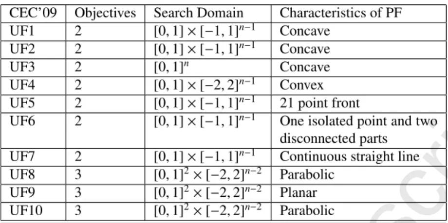
Due to the flurry of MOEAs recently developed, their performances are measured on diﬀerent MOP test suites, some related to real-world applications, while most were generated for testing purposes. Several such test suites comprising unconstrained (but bound constrained) as well as constrained problems have been presented in special sessions at events such as the CEC 09. This particular one provides performance assessment guidelines and code in web-sites such as http://dces.essex.ac.uk/staﬀ/qzhang/moeacompetition09.htm. Table 1 records the statistics of the ten unconstrained CEC’09 test instances [74] used in our experiments.

4.1. Parameter Settings

The following parameter values have been used in our experiments.

• N=600 for 2-objective test instances;

• N=1000 for 3-objective test instances;

• T =0.1Nare closest weight vectors;

• nr=0.01Nis the maximum number of solutions replaced by each new solution;

(8)

Accepted Manuscript

Table 1. IEEE CEC’09 Benchmark Functions Characteristics.

CEC’09 Objectives Search Domain Characteristics of PF UF1 2 [0,1]×[−1,1]n−1 _Concave

UF2 2 [0,1]×[−1,1]n−1 _Concave

UF3 2 [0,1]n _Concave

UF4 2 [0,1]×[−2,2]n−1 Convex UF5 2 [0,1]×[−1,1]n−1 _{21 point front}

UF6 2 [0,1]×[−1,1]n−1 One isolated point and two disconnected parts

UF7 2 [0,1]×[−1,1]n−1 _{Continuous straight line}

UF8 3 [0,1]2×[−2,2]n−2 Parabolic UF9 3 [0,1]2_×_[₋₂_,_2]n−2 _Planar

UF10 3 [0,1]2×[−2,2]n−2 Parabolic

• δ=0.9 is the probability with regard to selecting P;

• η=20 andpm=1/nin the polynomial mutation operator;

• ADE parameterCR=F=0.5∗(1+rand), whererand()∈[0,1];

• The maximum number of function evaluations is 300,000; 4.2. Weight Vector Selection

A set ofNweight vectors,W, is generated according to the following procedure [73]:

1. Uniformly randomly generate 5,000 weight vectors to form setW1. SetW is initialised with weight vectors

(1,0, . . . ,0,0), (0,1, . . . ,0,0), . . . , (0,0, . . . ,0,1);

2. Find the weight vector in setW1with the largest distance to setW; include it in setW and remove it from set

W1.

3. If|W|=N, stop and return it. Else, go to 2. 4.3. Performance Indicators

Two main goals must be kept in sight when dealing with MOP. They are: 1. the convergence towards the Pareto-optimal front,

2. the uniformity and good distribution of the set of multiple solutions that cover the true PF of the problem in hand [11].

Several performance metrics found in the specialized literature on evolutionary computing (EC) [65, 13, 11, 81] are used to rank algorithms in terms of performance. They are the inverted generational distance (IGD), [81, 74], the relative HYPer-volume (HYP), [65, 11], the Gamma (Γ) and Delta (∆) indicators, [11, 13]; they are commonly used in several comparative analyses of a variety of algorithms. These performance indicators can only be used if the reference set of the problem at hand is known in advance or is available with the test suites. In this paper, we have used the following performance indicators.

(9)

Accepted Manuscript

4.3.1. The Inverted Generational Distance (IGD)

LetP∗be a set of uniformly distributed points along the PF. LetAbe an approximate set of the PF, the average distance fromP∗toAis defined as [74]:

D(A,P)=

∑

v∈P∗d(v,A)

|P∗| ,

whered(v,A) is the minimum Euclidean distance betweenvand the points inA. IfP∗ is large enough to represent the PF very well, thenD(A,P) could measure both the diversity and convergence ofAin a sense. The closer the IGD metric values, the better the approximation set is. We have usedP∗=500 in our experiments to tackle 2-objective test instances andP∗=1000 to solve 3-objective problems.

4.3.2. The Relative Hyper-volume Indicator (HYP) HYP is mathematically expressed as

HY P(A)= HV(P

∗₎₋_HV(A) HV(P∗) ,

whereHVdenotes the hyper-volume of the approximate setAofP∗and it is calculated as follows, [65, 66]: HV(A)=volume∪|_iA₌|₁zi

wherei∈Aandziis theithhypercube constructed with respect to reference pointWand the solutionias the diagonal

corners of the hypercube. The closer the value of HYP to zero, the closer the approximate set of solutions to the true Pareto-optimal set.

4.3.3. The Gamma (Γ) Performance Indicator

To use theΓ metric [13], we generateP∗ =500 uniformly spaced solutions from the true Pareto optimal front in the objective space of the problem at hand to calculate theΓ metric values. Then, we compute the minimum Euclidean distance of each individual solution belonging to the approximated set of solutions denoted byAbetween P∗the Pareto-optimal solutions. The average of these distances represents theΓmetric values. In practice, if theΓ metric value is close to zero, the approximate set will converge well to the true Pareto front. This metric measures the extent of convergence to a known set of Pareto-optimal solutions. However, it fails to provide complete information about the spread in the obtained solutions. For this reason, we use another metric denoted∆which is explained below. 4.3.4. The Delta (∆) Performance Indicator

∆is a metric function calculated as follows, [13].

∆ = df+dI+ ∑N₋1

i=1 di−d

df +dI+(N−1)d ,

wheredf anddIare the Euclidean distances of the extreme and the boundary solutions belonging to the approximate

set of the optimal solutions set andddenotes the average of all Euclidean distancesdibetween consecutive solutions

in the final approximate set of optimal solutions provided by a particular algorithm.

5. Experimental Results: Discussion

The experiments have been carried out on the following computing platform and parameter values.

• Operating system: Windows XP Professional;

• Programming language: Matlab;

• CPU: Core 2 Quad 2.4 GHz;

• RAM: 4 GB DDR2 1066 MHz;

(10)

Accepted Manuscript

• Execution: 30 times each algorithm with diﬀerent random seeds;

In our experimental investigation, first we have embedded some crossover operators, namely, CMX [61, 62], ADE [53], PCX [12], and TM [17], one by one in MOEA/D, [73] without any modification of the original framework. As a result MOEA/D-CMX, MOEA/D-ADE, MOEA/D-PCX and MOEA/D-TM have been developed and form the core matter of this paper.

Secondly, we developed HAEA/D by enhancing MOEA/D [73] with the four cross-overs mentioned above. Each used crossover receives resources based on the performance of its generated individuals/solutions within the HAEA/D framework. This performance is in terms of the fitness values of the parents allocated to each crossover and the oﬀspring produced by a given crossover. HAEA/D and the other considered algorithms have been executed with the same parameter settings as explained in Section 4.1 and their algorithmic behaviors have been investigated thoroughly using four diﬀerent indicators as explained in Section 4.3.1.

The IGD-metric values obtained by HAEA/D and four other versions of MOEA/D [73] on each of UF1 through to UF10 problems, are recorded in Table 2 and Table 3. The 1stcolumn in each of these tables shows the minimum (Min), the 2nd_{the maximum (Max), the 3}rd_{the mean, and the 4}th_{column shows the standard deviation (Std) of}

IGD-metric values. From these tables one can conclude that HAEA/D has found a better approximate set of solutions with minimum average IGD-values compared to the other algorithms on most CEC’09 test instances, [74].

The last columns of Tables 2 and 3, indicate that the experimental results obtained with all algorithms for instances UF5 and UF6 are not good due to the fact that the objective function profiles of these problems are very complicated; small perturbations in the data have a big eﬀect on the populations of solutions generated by these algorithms and cause them to be dominated and/or get stuck in the local basins of attraction of some solutions. Note also that HAEA/D does not allow evolved solutions to replace allT neighbouring solutions as in the original MOEA/D, [72]. The mating restriction in HAEA/D, a type of elitism, which prevents promising solutions from taking part in the process of evolution, may have a drawback. However, mating restriction strategies are quite useful in that they improve the time complexity of algorithms.

Table 4 shows the IGD-metric values produced by A) MTS, [60], B) GDE3, [32], C) DECMOSA-SQP, [70], algorithms to cope with UF1-UF10 test instances. Among all these algorithms, MTS has handled both UF1 and UF6 with minimum IGD-values over 30 independent runs as compared to GDE3, DECMOSA-SQP, HAEA/D and four other diﬀerent versions of MOEA/D [73] considered in this paper.

Table 5 presents the values of the relative hypervolume (HYP) in the 1st_row,_Γ_{in the 2}nd _and_∆_{in the 3}rd_{, for}

each of UF1 to UF10, respectively. Columns 1st_{, through to 5}th_{of this table lists the best, median, average, standard}

deviation (std) and maximum values of the relative hypervolume, Γ and∆ indicators, respectively. The average variation accrued in the values of these indicators are displayed in Figures 8, 9 and 10 which clearly demonstrate that HAEA/D has performed well on most CEC’09 test instances as compared to the four diﬀerent versions of MOEA/D [73] based on a single crossover with average indicator values.

The best PFs of some CEC’09 test instances, [74] with respect to a) HAEA/D, b) MOEA/D-CMX, c) MOEA/ D-ADE, d) MOEA/D-PCX, e) MOEA/D-TM are shown in Figures 1, 2 and 3. One can see from these figures that the proposed algorithm has found better a PF for most test instances with good convergence and diversity as compared to the MOEA/D versions. Note that we did not include the figures corresponding to MOEA/D-PCX and MOEA/D-TM to keep down the volume of the paper.

In Figures 4, 5 and 6, we have plotted all 30 PFs together to show the distribution ranges of the final populations approximated by the above mentioned algorithms in 30 independent runs on CEC’09 test instances. The figures clearly demonstrate that HAEA/D has found better solutions in terms of the distribution ranges compared to the ones generated by the algorithms used in the comparative investigation.

The average IGD-metric values are plotted against the number of generations in Figure 7. This figure shows that HAEA/D has solved most problems with minimum average IGD-metric value as compared to most of the algorithms considered here.

5.1. Statistical Significance Analysis of the HAEA/D

In order to have statistically sound conclusions, we conducted the Wilcoxons rank sum tests at 0.05 significance level aim at establishing significance diﬀerences between the suggested algorithm and the rest of the state-of-the-art MOEAs considered. In this regard, the IGD-metric values of the suggested algorithm are used along with the other

(11)

Accepted Manuscript

used MOEAs to assign them ranks according to their performance, where the last columns of Tables 2, 3 and 4 provide details regarding the ranks of each MOEA. We have highlighted the best ranking MOEA in bold in the mentioned tables.

Table 2. IGD-metric values of A) HAEA/D, B) MOEA/D-CMX, C) MOEA/D-ADE, D) MOEA/D-PCX), E) MOEA/D-TM, F) MOEA/D-DE+PSO [44], G) MOEA/D-CPDE [34] when applied to UF1-UF5 of the IEEE CEC09 test instances [74].

CEC’09 Min Median Mean Std Max EAs RK

UF1 0.003943 0.004253 0.004275 0.000222 0.00494 A 1 0.004178 0.004589 0.005397 0.003487 0.022876 B 4 0.004847 0.010675 0.010995 0.003732 0.019072 C 6 0.031234 0.063827 0.074934 0.037351 0.188678 D 9 0.044052 0.077233 0.072754 0.017260 0.113685 E 8 0.004466 0.0182737 0.0285723 0.02360902 0.0711827 F 7 0.004594 - 0.005203 0.000248 0.006144 G 2 UF2 0.004135 0.004125 0.004138 0.000715 0.009050 A 1 0.005287 0.006875 0.006958 0.001154 0.009084 B 4 0.004580 0.005584 0.00653 0.001551 0.010123 C 3 0.010176 0.018078 0.020656 0.010734 0.047623 D 8 0.024549 0.029689 0.031660 0.006182 0.053112 E 10 0.010218 0.011671 0.011737 0.000756 0.013261 F 5 0.008998 - 0.011877 0.001714 0.015334 G 6 UF3 0.004043 0.021355 0.021138 0.020926 0.059050 A 2 0.004454 0.022377 0.032645 0.027109 0.091392 B 3 0.006955 0.0468554 0.044923 0.02754 0.09362 C 4 0.114871 0.206634 0.204245 0.038934 0.269345 D 8 0.031612 0.694083 1.665783 4.869497 24.661914 E 10 0.0039404 0.0058284 0.006039 0.001826 0.010494 F 1 0.008435 - 0.044706 0.029862 0.114730 G 5 UF4 0.039089 0.045792 0.047761 0.007650 0.062431 A 6 0.053578 0.060667 0.061493 0.004765 0.073944 B 9 0.041028 0.048083 0.049150 0.005221 0.062834 C 7 0.049639 0.056073 0.058145 0.007545 0.078592 D 8 0.047843 0.054604 0.0040458 0.004053 0.071241 E 1 0.043632 - 0.045344 0.001319 0.049677 G 5 UF5 0.188700 0.242179 0.295313 0.118853 0.707107 A 6 0.222475 0.383753 0.425495 0.154682 0.712491 B 8 0.127310 0.270832 0.281138 0.087448 0.480059 C 5 0.170921 0.379723 0.378716 0.0131373 0.643197 D 7 0.200144 0.417523 0.458011 0.139898 0.822995 E 9 0.282111 0.454364 0.490882 0.118561 0.708999 F 10 0.115859 - 0.203445 0.045309 0.258254 G 4 10

(12)

Accepted Manuscript

Table 3. IGD-metric values of A) HAEA/D, B) MOEA/D-CMX, C) MOEA/D-ADE, D) MOEA/D-PCX), E) MOEA/D-TM, F) MOEA/D-DE+PSO [44], G) MOEA/D-CPDE [34] when applied to UF6-UF10 of IEEE CEC09 test instances [74].

CEC’09 Min Median Mean Std Max EAs RK

UF6 0.051234 0.173364 0.196282 0.101955 0.474144 A 5 0.150081 0.443699 0.398187 0.153898 0.761923 B 9 0.041672 0.0902887 0.0903197 0.030015 0.250136 C 2 0.077549 0.204678 0.284849 0.205672 0.832798 D 7 0.193984 0.399496 0.390574 0.128275 0.727768 E 8 0.186140 0.823351 0.778214 0.157339 0.843885 F 10 0.073819 - 0.091573 0.030068 0.210588 G 3 UF7 0.004549 0.005769 0.005988 0.001489 0.012287 A 1 0.004884 0.006387 0.008573 0.005581 0.031779 B 2 0.004898 0.008514 0.009190 0.003596 0.023703 C 3 0.012956 0.114638 0.190943 0.195067 0.619975 D 8 0.017341 0.024890 0.144043 0.154892 0.495634 E 9 0.006726 0.008776 0.243517 0.237355 0.674953 F 10 0.005112 - 0.006067 0.000640 0.007461 G 7 UF8 0.058455 0.074751 0.082124 0.018202 0.125892 A 3 0.058878 0.068588 0.075276 0.016682 0.101398 B 1 0.086072 0.088657 0.087818 0.006782 0.102548 C 4 0.891378 1.016922 1.009308 0.066704 1.117835 D 9 1.187237 1.370320 1.368381 0.074510 1.516075 E 10 0.057600 0.076222 0.078455 0.006532 0.1019020 F 2 0.112641 - 0.123347 0.006231 0.139016 G 5 UF9 0.039255 0.122295 0.107791 0.052809 0.175837 A 5 0.049189 0.151583 0.128087 0.060854 0.325666 B 8 0.043128 0.069057 0.087238 0.042770 0.177565 C 4 0.096845 0.18768 0.170278 0.036245 0.219371 D 9 0.207515 0.287547 0.280701 0.046702 0.343331 E 10 0.035499 0.038980 0.071131 0.035008 0.149478 F 1 0.074763 - 0.080028 0.002555 0.083058 G 2 UF10 0.282175 0.413275 0.421193 0.059551 0.545143 A 6 0.428067 0.478093 0.484467 0.035198 0.553108 B 8 0.215141 0.344499 0.372537 0.107854 0.627219 C 4 0.195734 0.402962 0.382064 0.147843 0.761573 D 5 0.417532 0.489873 0.494567 0.046058 0.599181 E 9 0.184050 0.187033 0.187158 0.001552 0.190097 F 2 0.369133 - 0.499921 0.078278 0.688156 G 10 11

(13)

Accepted Manuscript

Table 4. IGD-metric values over 30 independent runs of (H) MTS [60],(I) GDE3 [32]and (J) DECMOSA-SQP [70] when applied to UF1-UF10 CEC’09 test instances [74].

H) MTS, I) GDE3, J) DECMOSA-SQP

CEC’09 Min Mean Std Max EAs RK

UF1 0.005782 0.006467 0.0003485 0.007221 H 5 0.004815 0.005342 0.000342 0.006242 I 3 0.055126 0.0770281 0.039379 0.0880129 J 10 UF2 0.005188 0.006157 0.000508 0.007499 H 2 0.009020 0.011953 0.001541 0.014972 I 7 0.017336 0.028342 0.031318 0.04022 J 9 UF3 0.037394 0.053107 0.0117366 0.077863 H 9 0.085759 0.106395 0.012900 0.138381 I 7 0.030545 0.093500 0.19795 0.16816 J 6 UF4 0.022486 0.023561 0.0006641 0.024950 H 3 0.025857 0.026506 0.000372 0.027550 I 2 0.031624 0.033926 0.005370 0.035643 J 4 UF5 0.009743 0.003277 0.0032771 0.022036 H 1 0.031791 0.039281 0.003947 0.045880 I 2 0.133012 0.167139 0.089508 0.237081 J 3 UF6 0.041631 0.059178 0.0106224 0.090268 H 1 0.204163 0.250913 0.019573 0.282468 I 6 0.057917 0.126042 0.561753 0.589904 J 4 UF7 0.015951 0.040794 0.0144456 0.081103 H 5 0.014125 0.025228 0.008891 0.042002 I 4 0.0198913 0.024163 0.022349 0.0427502 J 6 UF8 0.090927 0.112517 0.0129335 0.138652 H 6 0.194990 0.248556 0.035521 0.365385 I 8 0.098938 0.215834 0.121475 0.228895 J 7 UF9 0.062463 0.114423 0.0254955 0.182694 H 6 0.045261 0.082482 0.022485 0.133812 I 3 0.062463 0.114423 0.0254955 0.182694 J 7 UF10 0.124504 0.153065 0.0158331 0.198014 H 1 0.393773 0.433261 0.012323 0.445574 I 7 0.238279 0.369857 0.65322 0.580852 J 3 12

(14)

Accepted Manuscript

Table 5. Relative hypervolume,Γand∆function values found by HAEA/D in 30 independent runs on UF1-UF10 CEC’09 test instances [74]. HYP: Relative Hypervolume,Γ: Gamma function,∆: Delta function

CEC’09 Min Median Mean Std Max Metrics

UF1 0.00220045 0.01255353 0.01202675 0.00535225 0.02275685 HYP 0.00121840 0.00174985 0.00180623 0.00022546 0.00238502 Γ 0.07801665 0.11353670 0.11433680 0.01288763 0.15680761 ∆ UF2 0.00291273 0.00465720 0.00843102 0.01004413 0.02768225 HYP 0.00203678 0.00218194 0.00180623 0.00265505 0.00715213 Γ 0.11293602 0.13404632 0.14648345 0.04293143 0.23655212 ∆ UF3 0.00004254 0.00014643 0.00053125 0.00264534 0.01403214 HYP 0.00121481 0.00242053 0.00430134 0.00656321 0.03284612 Γ 0.07029556 0.10969542 0.10161512 0.08430107 0.50246075 ∆ UF4 0.00598240 0.55587351 0.60157204 0.32040712 0.83525984 HYP 0.04764373 0.05537687 0.05456813 0.00326493 0.06052927 Γ 0.12937862 0.23535025 0.23170045 0.04069459 0.30314138 ∆ UF5 0.00598240 0.65587451 0.60247204 0.35000214 0.78654364 HYP 0.79072623 0.81263565 0.81472453 0.91047034 0.98745035 Γ 0.98730817 0.82635653 0.83724536 0.86547032 0.98748051 ∆ UF6 0.02205605 0.37265342 0.40516564 0.20103465 0.85639675 HYP 0.00010862 0.08427560 0.07814091 0.05140101 0.19555661 Γ 0.87963604 0.90446772 0.90248338 0.08398419 0.93354324 ∆ UF7 0.00043681 0.00516514 0.00475982 0.00763563 0.03453752 HYP 0.00105175 0.00170317 0.00172401 0.00047320 0.00323692 Γ 0.06703412 0.09153683 0.08672308 0.04332503 0.25342028 ∆ UF8 0.87601574 0.85057461 0.84050834 0.00060703 0.89179615 HYP 0.01510523 0.03068203 0.03202178 0.03741104 0.17045402 Γ 0.01716533 0.04068203 0.04310127 0.04230103 0.18079422 ∆ UF9 0.86172901 0.87114726 0.87139222 0.00356474 0.98670624 HYP 0.08674953 0.20654221 0.21256451 0.17921201 0.09908802 Γ 0.45456348 0.66454237 0.57154904 0.08541573 0.83435762 ∆ UF10 0.87004740 0.87389041 0.86918374 0.00210681 0.91342709 HYP 0.04122707 0.50831050 0.51040308 0.41692692 0.09303015 Γ 0.5487735 0.71304252 0.71140378 0.13701056 0.61245170 ∆ 13

(15)

Accepted Manuscript

0.0 0.2 0.4 0,6 0.8 1.0 1.2 0.0 0.2 0.4 0,6 0.8 1.0 1.2 f1 f2

Pareto Front of UF1 True PF HAEA/D 0.0 0.2 0.4 0,6 0.8 1.0 1.2 0.0 0.2 0.4 0,6 0.8 1.0 1.2 f1 f2

Pareto Front of UF7 True PF HAEA/D 0.00.20.40,6 0.81.01.2 0.0 0.2 0.4 0,6 0.8 1.0 1.2 0.0 0.2 0.4 0,6 0.8 1.0 1.2 f1 Pareto Front of UF8

f2 f3 True PF HAEA/D 0.00.20.40,6 0.81.01.2 0.0 0.2 0.4 0,6 0.8 1.0 1.2 0.0 0.2 0.4 0,6 0.8 1.0 1.2 f1 Pareto Front of UF9

f2 f3 True PF HAEA/D 0.00.20.40,6 0.81.01.2 0.0 0.2 0.4 0,6 0.8 1.0 1.2 0.0 0.2 0.4 0,6 0.8 1.0 1.2 f1 Pareto Front of UF10

f2

f3

True PF HAEA/D

Figure 1. Plots of the approximated Pareto Fronts of the best run among 30 independent runs of HAEA/D on CEC’09 test instances [74].

0.0 0.2 0.4 0,6 0.8 1.0 1.2 0.0 0.2 0.4 0,6 0.8 1.0 1.2 f1 f2

Pareto Front of UF1 True PF MOEA/D−CMX 0.0 0.2 0.4 0,6 0.8 1.0 1.2 0.0 0.2 0.4 0,6 0.8 1.0 1.2 f1 f2

Pareto Front of UF7 True PF MOEA/D−CMX 0.00.20.40,6 0.81.01.2 0.0 0.2 0.4 0,6 0.8 1.0 1.2 0.0 0.2 0.4 0,6 0.8 1.0 1.2 f1 Pareto Front of UF8

f2 f3 True PF MOEA/D−CMX 0.00.20.40,6 0.81.01.2 0.0 0.2 0.4 0,6 0.8 1.0 1.2 0.0 0.2 0.4 0,6 0.8 1.0 1.2

Pareto Front of UF9

f1 f2 f3 True PF MOEA/D−CMX 0.00.20.40,6 0.81.01.2 0.0 0.2 0.4 0,6 0.8 1.0 1.2 0.0 0.2 0.4 0,6 0.8 1.0 1.2 f1 Pareto Front of UF10

f2

f3

True PF MOEA/D−CMX

Figure 2. Plots of the approximated Pareto Fronts of the best run among 30 independent runs of MOEA/D-CMX on CEC’09 test instances [74].

(16)

Accepted Manuscript

0.0 0.2 0.4 0,6 0.8 1.0 1.2 0.0 0.2 0.4 0,6 0.8 1.0 1.2 f1 f2

Pareto Front of UF1 True PF MOEA/D−ADE 0.0 0.2 0.4 0,6 0.8 1.0 1.2 0.0 0.2 0.4 0,6 0.8 1.0 1.2 f1 f2

Pareto Front of UF7 True PF MOEA/D−ADE 0.00.20.40,6 0.81.01.2 0.0 0.2 0.4 0,6 0.8 1.0 1.2 0.0 0.2 0.4 0,6 0.8 1.0 1.2 f1 Pareto Front of UF8

f2 f3 True PF MOEA/D−ADE 0.00.20.40,6 0.81.01.2 0.0 0.2 0.4 0,6 0.8 1.0 1.2 0.0 0.2 0.4 0,6 0.8 1.0 1.2 f1 Pareto Front of UF9

f2 f3 True PF MOEA/D−ADE 0.00.20.40,6 0.81.01.2 0.0 0.2 0.4 0,6 0.8 1.0 1.2 0.0 0.2 0.4 0,6 0.8 1.0 1.2 f3 f1 Pareto Front of UF10

f2

True PF MOEA/D−ADE

Figure 3. Plots of the approximated Pareto Fronts of the best run among 30 independent runs of MOEA/D-ADE on CEC’09 test instances [74].

0.0 0.2 0.4 0,6 0.8 1.0 1.2 0.0 0.2 0.4 0,6 0.8 1.0 1.2 f1 f2

Thirty Pareto Fronts of UF1 altogather against true Pareto Front. True PF HAEA/D 0.0 0.2 0.4 0,6 0.8 1.0 1.2 0.0 0.2 0.4 0,6 0.8 1.0 1.2 f1 f2

Thirty Pareto Fronts of UF7 altogather against true Pareto Front. True PF HAEA/D 0.00.20.40,60.81.01.2 0.0 0.2 0.4 0,6 0.8 1.0 1.2 0.0 0.2 0.4 0,6 0.8 1.0 1.2 f1 Thirty Pareto Fronts of UF8 altogather against true Pareto Front.

f2 True PF HAEA/D 0.00.20.40,60.81.01.2 0.0 0.2 0.4 0,6 0.8 1.0 1.2 0.0 0.2 0.4 0,6 0.8 1.0 1.2

Thirty Pareto Fronts of UF9 altogather against true Pareto Front.

f1 f2 True PF HAEA/D 0.00.20.40,60.81.01.2 0.0 0.2 0.4 0,6 0.8 1.0 1.2 0.0 0.2 0.4 0,6 0.8 1.0 1.2 f1 Thirty Pareto Fronts of UF10 altogather against true Pareto Front.

f2

True PF HAEA/D

Figure 4. Plots of the 30 approximated Pareto Fronts found by HAEA/D on CEC’09 test instances, [74].

(17)

Accepted Manuscript

0.0 0.2 0.4 0,6 0.8 1.0 1.2 0.0 0.2 0.4 0,6 0.8 1.0 1.2 f1 f2

Thirty Pareto Fronts of UF1 altogather against true Pareto Front. True PF MOEA/D−CMX 0.0 0.2 0.4 0,6 0.8 1.0 1.2 0.0 0.2 0.4 0,6 0.8 1.0 1.2 f1 f2

Thirty Pareto Fronts of UF7 altogather against true Pareto Front. True PF MOEA/D−CMX 0.00.20.40,60.81.01.2 0.0 0.2 0.4 0,6 0.8 1.0 1.2 0.0 0.2 0.4 0,6 0.8 1.0 1.2 f1 Thirty Pareto Fronts of UF8 altogather against true Pareto Front.

f2 True PF MOEA/D−CMX 0.00.20.40,60.81.01.2 0.0 0.2 0.4 0,6 0.8 1.0 1.2 0.0 0.2 0.4 0,6 0.8 1.0 1.2

Thirty Pareto Fronts of UF9 altogather against true Pareto Front.

f1 f2

True PF MOEA/D−CMX

Figure 5. Plots of the 30 approximated Pareto Fronts found by MOEA/D-CMX for CEC’09 test instances, [74].

0.0 0.2 0.4 0,6 0.8 1.0 1.2 0.0 0.2 0.4 0,6 0.8 1.0 1.2 f1 f2

Thirty Pareto Fronts of UF1 altogather against true Pareto Front. True PF MOEA/D−ADE 0.0 0.2 0.4 0,6 0.8 1.0 1.2 0.0 0.2 0.4 0,6 0.8 1.0 1.2 f1 f2

Thirty Pareto Fronts of UF7 altogather against true Pareto Front. True PF MOEA/D−ADE 0.00.20.40,60.81.01.2 0.0 0.2 0.4 0,6 0.8 1.0 1.2 0.0 0.2 0.4 0,6 0.8 1.0 1.2 f1 Thirty Pareto Fronts of UF8 altogather against true Pareto Front.

f2 True PF MOEA/D−ADE 0.00.20.40,60.81.01.2 0.0 0.2 0.4 0,6 0.8 1.0 1.2 0.0 0.2 0.4 0,6 0.8 1.0 1.2 f1 Thirty Pareto Fronts of UF9 altogather against true Pareto Front.

f2 True PF MOEA/D−ADE 0.00.20.40,60.81.01.2 0.0 0.2 0.4 0,6 0.8 1.0 1.2 0.0 0.2 0.4 0,6 0.8 1.0 1.2 f1 Thirty Pareto Fronts of UF10 altogather against true Pareto Front.

f2

True PF MOEA/D−ADE

Figure 6. Plots of 30 approximate Pareto Fronts found by MOEA/D-ADE for CEC’09 test instances, [74].

(18)

Accepted Manuscript

0 100 200 300 400 500 10−3 10−2 10−1 100 101 UF1 Function Evaluations

Averge Variation in IGD Values

HAEAD MOEA/D−CMX MOEA/D−ADE MOEA/D−PCX MOEA/D−TRIG−MUT 0 100 200 300 400 500 10−3 10−2 10−1 100 UF2 Function Evaluations

HAEAD MOEA/D−CMX MOEA/D−ADE MOEA/D−PCX MOEA/D−TRIG−MUT 0 100 200 300 400 500 10−2 10−1 100 101 UF3 Function Evaluations

HAEAD MOEA/D−CMX MOEA/D−ADE MOEA/D−PCX MOEA/D−TRIG−MUT 0 100 200 300 400 500 100 UF5 Function Evaluations

HAEAD MOEA/D−CMX MOEA/D−ADE MOEA/D−PCX MOEA/D−TRIG−MUT 0 100 200 300 400 500 10−3 10−2 10−1 100 101 UF7 Function Evaluations

HAEAD MOEA/D−CMX MOEA/D−ADE MOEA/D−PCX MOEA/D−TRIG−MUT 0 50 100 150 200 250 300 10−2 10−1 100 101 UF8 Function Evaluations

HAEAD MOEA/D−CMX MOEA/D−ADE MOEA/D−PCX MOEA/D−TRIG−MUT

Figure 7. Plots of the final solutions with lowest IGD values found by HAEA/D, MOEA/D-CMX, MOEA/D-ADE,MOEA/D-PCX and MOEA/ D-TM in 30 independent runs on CEC’09 test instances, [74].

Averge Relative Hypervolume Deviation

HAEAD MOEA/D−CMX MOEA/D−ADE MOEA/D−PCX MOEA/D−TRIG−MUT

Figure 8. Plots of the final solutions with the lowest Relative Hypervolume values found by HAEA/D, MOEA/D-CMX, MOEA/D-ADE, MOEA/ D-PCX and MOEA/D-TM in 30 independent runs on CEC’09 test instances, [74].

(19)

Accepted Manuscript

Averge Deviation in Gamma function Value

HAEAD MOEA/D−CMX MOEA/D−ADE MOEA/D−PCX MOEA/D−TRIG−MUT

Figure 9. Plots of the final solutions with the lowestΓfunction values found by HAEA/D, MOEA/D-CMX, MOEA/D-ADE, MOEA/D-PCX and MOEA/D-TM in 30 independent runs on CEC’09 test instances [74].

Averge Deviation in Delata function Value

HAEAD MOEA/D−CMX MOEA/D−ADE MOEA/D−PCX MOEA/D−TRIG−MUT

Figure 10. Plots of the final solutions with the lowest∆function values found by HAEA/D, MOEA/D-CMX, MOEA/D-ADE, MOEA/D-PCX and MOEA/D-TM in 30 independent runs on CEC’09 test instances, [74].

5.2. Sensitivity of Population Size N and Neighbourhood Size T in HAEA/D

The neighbourhood sizeT is one of the most important parameters in HAEA/D. Its setting is based on population sizeNas in MOEA/D [72, 73, 33]. It is, therefore, important to study its impact when diﬀerent population sizesNare used in the HAEA/D framework. The last columns of Tables 6 and 7 provide the diﬀerent values ofNandT used to obtain the recorded IGD-metric values corresponding to the solutions returned by HAEA/D on CEC’09 test instances. Note that all other parameters are as explained in Section 4.1 when the algorithm is run 30 times independently over each CEC’09 test problem [74]. In general, as clearly shown in Figure 11, the performance of the suggested algorithm gets better with large size populations and high neighbourhood sizes.

(20)

Accepted Manuscript

Table 6. IGD-metric values for solutions found by HAEA/D with diﬀerent values ofNapplied to CEC’09 test instance [74].

CEC’09 Min Median Mean Std Max N T

UF1 0.0154861 0.043135 0.043793 0.0364123 0.150717 100 10 0.011752 0.0097635 0.009703 0.034175 0.137849 200 20 0.004129 0.005037 0.006873 0.007852 0.046767 300 30 0.003803 0.006011 0.0060303 0.0075932 0.046752 400 40 0.004017 0.005767 0.005690 0.002031 0.010453 500 50 UF2 0.0109156 0.013032 0.013201 0.001016 0.017311 100 10 0.007832 0.010328 0.012010 0.001002 0.015842 200 20 0.006134 0.004357 0.005265 0.000897 0.006245 300 30 0.006223 0.004343 0.004427 0.000619 0.010179 400 40 0.005304 0.004378 0.004231 0.000602 0.008324 500 50 UF3 0.047194 0.05124 0.051419 0.061489 0.125030 100 10 0.045174 0.0472456 0.050420 0.06035 0.122030 200 20 0.004188 0.02404 0.0245372 0.025863 0.086023 300 30 0.004075 0.023814 0.024143 0.020288 0.0.71245 400 40 0.004654 0.022030 0.022021 0.006756 0.034507 500 50 UF4 0.066031 0.080604 0.080407 0.008061 0.105614 100 10 0.050347 0.053500 0.053462 0.004838 0.071733 200 20 0.05036 0.013207 0.013301 0.015603 0.071123 300 30 0.057589 0.060794 0.01120 0.005536 0.083088 400 40 0.050508 0.015137 0.010154 0.004771 0.071678 500 50 UF5 0.3547931 0.526634 0.523743 0.127420 0.770570 100 10 0.324541 0.400737 0.410643 0.116410 0.702550 200 20 0.304162 0.361650 0.369325 0.070253 0.640103 300 30 0.26791 0.377591 0.369084 0.070084 0.630531 400 40 0.213475 0.353221 0.361207 0.069768 0.608106 500 50 19

(21)

Accepted Manuscript

Table 7. IGD-metric values for HAEA/D with diﬀerent values ofNwhen applied to CEC’09 test instance [74].

CEC’09 Min Median Mean Std Max N T

UF6 0.163743 0.430572 0.430632 0.132023 0.703027 100 10 0.153843 0.423102 0.423134 0.132012 0.702076 200 20 0.154252 0.420657 0.42101 0.130392 0.702004 300 30 0.150471 0.407079 0.408064 0.130553 0.700130 400 40 0.143015 0.412482 0.308267 0.123729 0.704633 500 50 UF7 0.008045 0.018031 0.181943 0.170417 0.534720 100 10 0.007012 0.07022 0.071020 0.163422 0.546720 200 20 0.005247 0.005635 0.006501 0.002456 0.016846 300 30 0.005969 0.005531 0.0055401 0.0024201 0.0142367 400 40 0.005032 0.005104 0.005201 0.001652 0.0140052 500 50 UF8 0.113042 0.132746 0.147027 0.034742 0.232342 100 10 0.102062 0.131764 0.132125 0.034664 0.230363 200 20 0.060263 0.088290 0.086985 0.034453 0.215247 500 50 0.051623 0.065814 0.066302 0.016072 0.130021 600 60 0.051145 0.065743 0.0655787 0.016023 0.130014 800 80 UF9 0.114720 0.201512 0.202102 0.023442 0.250684 100 10 0.114617 0.201302 0.202113 0.023488 0.260696 200 20 0.057576 0.152300 0.154230 0.0230373 0.189787 500 50 0.057067 0.152041 0.151974 0.032441 0.118181 600 60 0.053023 0.076842 0.07720 0.020167 0.10234 800 80 UF10 0.427416 0.510471 0.512021 0.056342 0.511059 100 10 0.426425 0.511302 0.512011 0.056472 0.511057 200 20 0.354046 0.456048 0.456202 0.045423 0.526323 500 50 0.353065 0.440197 0.445363 0.037592 0.520965 600 60 0.314561 0.436521 0.436701 0.044025 0.530024 800 80 20

(22)

Accepted Manuscript

100 150 200 250 300 350 400 450 500 550 600 0 0.005 0.01 0.015 0.02 0.025 0.03 0.035 0.04 0.045 N: Population Size

Average evolution in IGD−mertic values

UF1 HAEA/D 100 150 200 250 300 350 400 450 500 550 600 4 5 6 7 8 9 10 11 12 13 14x 10 −3 N: Population Size

UF2 HAEA/D 100 150 200 250 300 350 400 450 500 550 600 0.02 0.025 0.03 0.035 0.04 0.045 0.05 0.055 N: Population Size

UF3 HAEA/D 100 150 200 250 300 350 400 450 500 550 600 0 0.01 0.02 0.03 0.04 0.05 0.06 0.07 0.08 0.09 N: Population Size

UF4 HAEA/D 100 150 200 250 300 350 400 450 500 550 600 0.25 0.3 0.35 0.4 0.45 0.5 0.55 0.6 N: Population Size

UF5 HAEA/D 100 150 200 250 300 350 400 450 500 550 600 0.2 0.25 0.3 0.35 0.4 0.45 0.5 N: Population Size

UF6 HAEA/D 100 150 200 250 300 350 400 450 500 550 600 0 0.02 0.04 0.06 0.08 0.1 0.12 N: Population Size

UF8 HAEA/D 100 150 200 250 300 350 400 450 500 550 600 0.06 0.08 0.1 0.12 0.14 0.16 0.18 0.2 0.22 0.24 N: Population Size

UF10

HAEA/D

Figure 11. The average IGD-metric value versus the value of population size in HAEA/D for CEC’09 test instances [74].

(23)

Accepted Manuscript

0 500 1000 1500 2000 2500 10−2 10−1 100 UF1

Maximum Number of Generations

The Proportion of Crossovers in HAEA/D.

ADE CMX SPX SBX 0 500 1000 1500 2000 2500 10−2 10−1 100 UF2

ADE CMX SPX SBX 0 500 1000 1500 2000 2500 10−2 10−1 100 UF4

ADE CMX SPX SBX 0 500 1000 1500 2000 2500 10−2 10−1 100 UF5

ADE CMX SPX SBX 0 500 1000 1500 2000 2500 10−2 10−1 100 UF6

ADE CMX SPX SBX 0 500 1000 1500 2000 2500 10−2 10−1 100 UF7

ADE CMX SPX SBX 0 500 1000 1500 10−2 10−1 100 UF8

ADE CMX SPX SBX 0 500 1000 1500 10−2 10−1 100 UF9

ADE CMX SPX SBX 0 500 1000 1500 10−2 10−1 100 UF10

ADE CMX SPX SBX

Figure 12. The proportion of crossover operators selected during the evolution process of HAEA/D applied to CEC’09 test problems. The implementation of the Adaptive Operators Selection (AOS) within Pareto dominance-based MOEAs is tedious and complex compared to implementing decomposition-based MOEA. The latter are more flexible and suitable as a framework in which to deploy multiple search operators. This is because improvements in the search are easier to measure by virtue of the basic concept of decomposability which allows to convert the given MOP into N scalar subproblems. In this paper, therefore, we have studied the eﬀect of the use of multiple search operators in adaptive and ensemble manner. In carried out experiment, we found that no single operator dominates the whole search process of the HAEA/D when applied to CEC’09 test instance [74].

Figure 12 demonstrates the eﬀect of the use of multiple search operators in adaptive and ensemble manner. It can be seen in these figures that no single operator dominates the whole search process of the HAEA/D when applied to CEC’09 test instance [74].

(24)

Accepted Manuscript

0 500 1000 1500 2000 2500

100 UF1

Number of Iterations

Average Utility Function Value

0 500 1000 1500 2000 2500

100 UF2

0 500 1000 1500 2000 2500

100 UF3

0 500 1000 1500 2000 2500

100 UF4

0 500 1000 1500 2000 2500

100 UF5

0 500 1000 1500 2000 2500

100 UF6

0 500 1000 1500 2000 2500

100 UF7

0 500 1000 1500

100 UF8

0 500 1000 1500

100 UF9

Figure 13. Dynamic evolution of the utility function values in HAEA/D when solving CEC’09 test problems.

Decomposition-based approaches convert the problem of approximating the PF intoNscalar optimization prob-lems (SOPs). These SOPs require diﬀerent amounts of computational resources. Figure 13 shows how the suggested HAEA/D algorithm allocates resources to each of theNsubproblems based on the measured improvement made by each solution in reducing the single objective function values.

6. Conclusion

Adaptive operator selection procedures employ multiple genetic operators and local search optimizers within an evolutionary algorithm framework to find the most suitable search operator for the given problems. A trial-and-error approach for MOEAs is unlikely to work. Engaging simultaneously various genetic operators not only improves the performance of the base line algorithm but also saves on the time that is necessary to find the operators that perform best in the diﬀerent stages of the optimization process. This paper proposes a hybrid adaptive evolutionary algorithm based on decomposition which employs multiple search operators in an MOEA/D framework based on a self-adaptive scheme. The proposed methodology allocates a population of solutions dynamically to each crossover operator based on their respective performances, to create new solutions. The overall performance of HAEA/D has been evaluated on

(25)

Accepted Manuscript

the CEC’09 test instances. The results have been compared to those of four diﬀerent versions of MOEA/D: MOEA/D with MTS, MOEA/D with GDE3, DECMOSA-SQP and MOEA/D-CPDE. Four diﬀerent performance indicators have been used in the comparative analysis.

HAEA/D has performed better on most CEC09 test instances in terms of proximity and diversity. These results suggest, therefore, that using adaptive genetic operators may be a good idea in other contexts. And using multiple solution approaches simultaneously as in the Multiple Algorithms Single Formulation paradigm or MAFS of [54] is worthwhile particularly when problem instances are new and the choice of appropriate algorithms for the given problems is not straightforward. Further investigation and testing is therefore warranted. In future, we also intend to test the performance of our suggested algorithm on dynamic multi-objective benchmarks developed for the sessions of the IEEE CEC’14 and IEEE CEC’15.

We also intend to investigative the algorithmic performance of our proposal on single objective constrained opti-mization problems. The basic idea is to convert a single objective constrained problem into a MOPs by treating the violation of constraints as an extra objective function.

7. Acknowledgment

We are grateful to Professor Qingfu Zhang of the Department of Mathematical Sciences of the University of Essex, UK for his valuable comments and discussion of the subject matter of this paper.

References

[1] A. Arias-Montano, C. A. Coello Coello, and E. Mezura Montes, “Multiobjective Evolutionary Algorithms in Aeronautical and Aerospace Engineering,”Evolutionary Computation, IEEE Transactions on, vol. 16, no. 5, pp. 662–694, 2012.

[2] A. Auger, J. Bader, D. Brockhoﬀ, and E. Zitzler, “Hypervolume-based multiobjective optimization: Theoretical foundations and Practical Implications,”Theoretical Computer Science, vol. 425, pp. 75–103, 2012.

[3] J. Bader and E. Zitzler, “HypE: An Algorithm for Fast Hypervolume-Based Many-Objective Optimization,”Evolutionary Computation, vol. 19, no. 1, pp. 45–76, 2011.

[4] H. J. C. Barbosa and A. Medeiros-E-Sa,On Adaptive Operator Probabilities in Real Coded Genetic Algorithms, 2000.

[5] N. Beume, B. Naujoks, and M. Emmerich, “SMS-EMOA: Multiobjective Selection based on Dominated hypervolume,”European Journal of Operational Research, vol. 181, no. 3, pp. 1653–1669, 2007.

[6] C. Coello and G. Lamont,Applications of Multi-objective Evolutionary Algorithms, ser. Advances in Natural Computation, 2004.

[7] C. A. C. Coello, G. B. Lamont, and D. A. V. Veldhuizen,Evolutionary Algorithms for Solving Multi-Objective Problems (Genetic and Evolutionary Computation). Secaucus, NJ, USA: Springer-Verlag New York, Inc., 2006.

[8] C. A. Coello Coello and R. L. Becerra, “Evolutionary Multiobjective Optimization in Materials Science and Engineering,”Materials and manufacturing processes, vol. 24, no. 2, pp. 119–129, 2009.

[9] C. A. Coello Coello, G. B.Lamont, and D. A. Veldhuizen,Evolutionary Algorithms for Solving Multi-Objective Problems. Kluwer Academic Publishers, New York,, March 2002.

[10] L. DaCosta, A. Fialho, M. Schoenauer, and M. Sebag, “Adaptive Operator Selection with Dynamic Multi-Armed Bandits,”GECCO, Atlanta, Georgia, USA, vol. 12, no. 16, pp. 913–920, July 2008.

[11] K. Deb,Multi-Objective Optimization Using Evolutionary Algorithms, 2nd ed., S. Ross and R. Weber, Eds. John Wiley and Sons Ltd, 2002. [12] K. Deb, A. Anand, and D. Joshi, “A Computationally Eﬃcient Evolutionary Algorithm for Real-Parameter Optimization ,”Evolutionary

Computation, vol. 10, pp. 371–395, 2002.

[13] K. Deb, A. Pratap, S. Agarwal, and T.Meyarivan, “A Fast and Elitist Multiobjective Genetic Algorithm:NSGA-II,”IEEE Transsation On Evolutionary Computation, vol. 6, no. 2, pp. 182–197, 2002.

[14] D.H.Phan and J.Suzuki, “R2-IBEA: R2 indicator based evolutionary algorithm for multiobjective optimization,” in2013 IEEE Congress on Evolutionary Computation (CEC), June 2013, pp. 1836–1845.

[15] D.Thierens, “An Adaptive Pursuit Strategy for Allocating Operator Probabilities,” inIn GECCO 05: Proceedings of the 2005 conference on Genetic and evolutionarycomputation, New York, NY, USA, 2005. ACM.2218, 2005, pp. 15391546,.

[16] R. Eberhart and J.Kennedy, “A New Optimizer Using Particle Swarm Theory,” inProceedings of the Sixth International Symposium on Micro Machine and Human Science, MHS’95, oct. 1995, pp. 39–43.

[17] H.-Y. Fan and J. Lampinen, “A Trigonometric Mutation Operation to Diﬀerential Evolution,”Journal of Global Optimization, vol. 27, no. 1, pp. 105–129, 2003.

[18] A. Fialho1, L. D. Costa, M. Schoenauer, and M. Sebag, “Extreme-Dynamic Multi-Armed Bandits for Adaptive Operator Selection,” in GECCO’09, Montreal Quebec, Canada, vol. 8, no. 12, July 2009, pp. 2213–2215.

[19] D. E. Goldberg,Genetic Algorithms in Search, Optimization and Machine Learning, 1st ed. Boston, MA, USA: Addison-Wesley Longman Publishing Co., Inc., 1989.

[20] ——, “Probability Matching, the Magnitude of Reinforcement, and Classifier System Bidding,”Machine Learning, vol. 5, no. 4, pp. 407–425, October 1990.

[21] J. Horn, N. Nafpliotis, and D. E. Goldberg., “A Niched Pareto Genetic Algorithm for Multiobjective Optimization,” inProceedings of the First IEEE Conference on Evolutionary Computation, CEC’94, 1994.

(26)