Adaptive underfrequency load shedding based on real time simulation

(1)

ADAPTIVE UNDERFREQUENCY LOAD SHEDDING BASED ON REAL TIME SIMULATION

By

Mosab Salah Aldeen Mohamed Zeyada

Approved:

Ahmed H. Eltom Gary Kobet

Professor of Electrical Engineering Adjunct Professor of Electrical Engineering

(Chair) (Committee Member)

Abdul Ofoli

Assistant Professor of Electrical Engineering

(2)

ii

ADAPTIVE UNDERFREQUENCY LOAD SHEDDING

BASED ON REAL TIME SIMULATION

By

Mosab Salah Aldeen Mohamed Zeyada

A Thesis Submitted to the Faculty of the University of Tennessee at Chattanooga in Partial Fulfillment

Of the Requirements for the Degree of Master of Science: Engineering

The University of Tennessee at Chattanooga Chattanooga, Tennessee

(3)

iii ABSTRACT

Conventional Underfrequency Load Shedding (UFLS) is used to balance generation and load when underfrequency conditions occur. It sheds a fixed, predetermined amount of load irrespective of disturbance location. Several adaptive UFLS schemes are proposed in the literature. Recent research discussed utilizing synchrophasor messages to implement adaptive UFLS but these studies have been using virtual PMUs. Of late, hardware implementations for adaptive UFLS scheme using actual Phasor Measurement Units (PMUs) are reported but also these studies are based on small power systems. This study presents hardware implementation of adaptive UFLS based on real time simulation of IEEE39-bus system.

The simulation tool used was OPAL-RT eMEGAsim real time digital simulator. To emulate the actual environment where the scheme could be used, a complete phasor network setup is established using actual devices, such as high accuracy Global Positioning System (GPS) clocks, PMUs and Synchrophasor Vector Processor (SVP).

The results obtained show that the adaptive UFLS scheme restored the frequency and curtailed the load based on voltage sag. Furthermore, the results are compared with conventional UFLS scheme.

(4)

iv

3. METHODOLOGY ...23

3.1 IEEE39-Bus System Model ...23

3.2 Equipment for the Implementation ...30

3.3 Software for the Implementation ...30

3.4 Amplifiers ...31

3.5 SEL-487E and 411L Relays...33

(5)

v

3.5.1.1 Global Setting ...34

3.5.1.2 Communication Port Setting ...37

3.6 SVP Program ...39

3.6.1 UFLS Main Program...39

3.7 Station Setup and Local Area Network ...42

4. RESULTS AND DISCUSSION ...44

4.1 Adaptive UFLS Results ...44

4.1.1 Test Case 1: Generator 5 Outage ...45

4.2 Discussion ...61

5. CONCLUSION AND FUTURE WORK ...64

5.1 Conclusion ...64 5.2 Future Work ...65 REFERENCES ...66 APPENDIX A. SYSTEM DATA ...68 VITA ...77

(6)

vi

LIST OF TABLES

2.1 Typical Conventional Load Shedding Stages ... 7

4.1 Adaptive UFLS Results for Case 1 ... 49

4.4 Comparison between Disturbance Power Computed by Matlab and SVP ... 62

4.5 Comparison of the Amount of Shed Power between Conventional UFLS and Adaptive UFLS ... 63

(7)

vii

LIST OF FIGURES

2.1 Adaptive UFLS algorithm flow chart………...12

2.2 Phasor network diagram………..……….…16

2.3 RT Lab simulation time step description ... 20

2.4 Overruns in real time simulation ... 20

2.5 Hardware in the loop (HIL) test ... 21

2.6 HIL test for adaptive UFLS scheme ... 22

3.1 IEEE39-bus system single line diagram ... 24

3.2 IEEE39-bus RT Lab model ... 26

3.3 RT Lab assignation of processors ... 27

3.4 Console subsystem ... 29

3.5 Connections between eMEGAsim analog outputs-Amplifier-Relays ... 32

3.6 PMU global setting ... 34

3.7 PMU general setting ... 36

3.8 Phasor data configuration ... 37

3.9 PMU port setting ... 38

3.10 COI frequency calculation in the SVP program ... 40

(8)

viii

4.2 Total disturbance power recorded in Matlab for case 1 ... 47

4.3 Total disturbance power estimated by the SVP for case 1 ... 47

4.4 Voltage dip and shed power for each load bus recorded in the SVP for case 1 ... 48

4.5 Frequency response without load shedding for case 1 ... 49

4.6 Frequency response with adaptive UFLS for case 1 ... 50

4.7 Frequency response with conventional UFLS for case 1 ... 51

4.13 Frequency response with conventional UFLS for case 2 ... 56

(9)

ix

LIST OF ABBREVIATIONS

AO, Analog Output

AGC, Automatic Generation Control

CAPE, Computer Aided Protection Engineering COI, Center of Inertia Frequency

DI, Digital Input

DPL, Distributed Parameters Line

GPS, Global Positioning System HIL, Hardware in the Loop

IEC, International Electro-technical Commission IEEE, Institute of Electrical and Electronics Engineers IED, Intelligent Electronic Device

LAN, Local Area Network.

NERC, North America Electric Reliability Council OUT, Output

PDC, Phasor Data Concentrator PLC, Programmable Logic Controller PMU, Phasor Measurement Unit RB, Remote Bit

SCADA, Supervisory Control and Data Acquisition SVP, Synchrophasor Vector Processor

(10)

x

SFR, System Frequency Response SPS, SimPower System

TCP, Transmission Control Protocol UFLS, Under-Frequency Load Shedding UDP, User Datagram Protocol

(11)

1 CHAPTER 1 INTRODUCTION

1.1General Description

Power system stability is defined as that property of a power system that enables it to remain in a state of operating equilibrium under normal operating conditions and to regain an acceptable state of equilibrium after being subjected to a disturbance (Kundur, Balu, & Lauby, 1994). The protection systems should be designed so that to take preventive actions when system contingencies (such as faults, major generators or lines outages) occur. However, preventive actions disrupt the power only in the affected area, and by doing so the rest of the power system remains in a stable condition.

Generally, power systems experience either frequency or voltage instability problem. If there is no action taken to recover the system to its normal state, pre-disturbance, the consequences can be catastrophic. In addition to that, a power system may experience a rotor angle instability which defined in (Kundur et al., 1994) as the ability of interconnected synchronous machines of a power system to remain in synchronism. In this study, only frequency instability is considered.

The frequency stability is normally associated with the balance between the real power generated and the real power required by the load. If the demand is significantly higher than the generation, the system will experience underfrequency conditions, and underfrequency load shedding (UFLS) relays should operate in order to bring the system frequency back to stable

(12)

2

conditions by shedding the load. On the other hand, if the generation is significantly higher than the load, the frequency of the system will increase, and overfrequency relays should operate to bring the frequency back to its normal value by tripping generator(s).

The power system frequency as well as voltage has a certain operating limits. The protection system should not operate when the system conditions lie within these allowable limits. Whenever these limits are not met, the associated protection system should operate. Under/over-frequency relays should operate whenever the system frequency is lower/higher than the minimum/maximum limits.

The utilities practice for UFLS is to shed, after a time delay, a fixed amount of load, from specified load buses whenever system frequency is lower than the threshold value. Such type of load shedding is called conventional UFLS. The conventional UFLS is inherently decentralized in nature, the shedding decision is distributed among the relays located in different areas, and it is usually implemented by frequency relays which are located in the load buses considered for load shedding.

The conventional UFLS is well known by utilities. In general, the setting for conventional UFLS relays is simple and consists only of two quantities, a set frequency and time delay. The main disadvantage of the conventional UFLS is that it sheds the same blocks of load irrespective of the disturbance location, rate of change of frequency and voltage dip at the load buses. Furthermore, since the amount of power to be shed in conventional UFLS is fixed, it may cause an overfrequency condition, because it may shed more or less power than the required amount. Therefore, to overcome the disadvantages of conventional UFLS an adaptive UFLS is proposed in (Seethalekshmi, Singh, & Srivastava, 2011). This study aims to test the adaptive UFLS scheme using actual industry devices.

(13)

3

The adaptive UFLS scheme was tested on New England 39-bus test system. It used the frequency and rate of change of frequency from the generator buses to compute the amount of disturbance power. In addition to that, it calculated the voltage dip based on the measurement received from load buses, and then it distributed the amount of power to be shed based on the calculated voltage dips at the load buses. The voltage dip was calculated from voltage magnitude before and after the disturbance instant.

Due to technology advancement, enhancement of communication infrastructures and deployment of Phasor Measurements Units (PMUs), monitoring of the system operation in real time in today’s power system could be possible. Moreover, from the valuable information being sent in real time to the control center, real time decision intended to take preventive actions to mitigate system blackouts could also be possible. The adaptive UFLS scheme proposed in (Seethalekshmi et al., 2011) is based on the availability of real time measurements from PMUs.

In the literature, the researchers assumed the availability of real time measurements in their work but they do not have actual PMUs data and a central processing unit to process the information and make decisions. In (Tang, Liu, Ponci, & Monti, 2013), adaptive UFLS and Under-Voltage Load Shedding (UVLS) scheme based on synchrophasor measurements was introduced. Although a real time digital simulator RTDS® was used as a testing platform to test the proposed adaptive scheme, there was no hardware central processing unit which is responsible for providing online assessment in real time of frequency stability condition of the system. Instead PMU cards from RTDS® Technologies were used to simulate the actual PMUs. Hence, each time a system disturbance scenario was carried out, a file was saved and loaded to Matlab where the program for load shedding was written and the analysis is performed offline.

(14)

4

In this study, a model of IEEE39-bus system is developed in OPAL-RT eMEGAsim real time digital simulator for HIL test, and actual GPS synchronized PMUs from SEL were used to provide online monitoring of the bus voltages of the IEEE39-bus system, by taking real time measurements from the analog output port of the simulator. Synchrophasor data are sent to SEL synchrophasor vector processor SVP using 60 msg/sec message rates through Ethernet cables. The SVP collects, time synchronizes, and processes these phasor measurements based on the load shedding program, adaptive UFLS, and accordingly sends trip signals to selected load buses to shed the load adaptively. The SVP monitors the system state after the load shedding to assure the system is operating in the stable conditions and within allowable limits. Although the adaptive UFLS scheme can be implemented as decentralized scheme, in this study a centralized scheme was considered by using central processing unit.

1.2Thesis Objective

The objective of this study is to implement a centralized adaptive UFLS scheme and test its validity using actual PMUs. Also the study aims to test the performance of the PMUs and the SVP when adaptive UFLS algorithm is implemented on them. Additionally, it also aims to validate the results obtained in (Abd Elwahid, 2013) for adaptive UFLS algorithm and obtain the response of the algorithm when tested in larger power system such as IEEE39-bus system.

The scheme was tested on the IEEE39-bus system using HIL test technology. Moreover, in this study a comparison between the performance of the conventional and adaptive UFLS schemes during underfrequency conditions was provided.

The study also aims to establish and test the performance of an actual phasor network consisting of PMUs, Global Positioning System (GPS) clocks and SVP. This is required to

(15)

5

emulate the real phasor network in modern power grid. These devices along with OPAL-RT eMEGAsim real time digital simulator are state of the art equipment which are used in cutting edge researches in the area of Wide Area Monitoring, Protection, and Control (WAMPC) application.

Furthermore, the study aims to build a model of IEEE39-bus system in eMEGAsim real time digital simulator, to be used as test bed for research and teaching purposes in the Smart Grid and protection laboratory at the University of Tennessee at Chattanooga. The main usage of the model is to perform hardware in the loop testing of new protection schemes especially, WAMPC applications. The model was built in different power system software, such as ETAP and CAPE, for conducting regular power system studies such as power flow, short circuits and coordination studies. On the other hand, for real time simulation purposes the model was built in RT lab and HYPERSIM software to aid in conducting hardware in the loop testing.

The model could also be used to test simple protection functions such as over-current, distance and differential, using hardware in the loop test technology. Since real time simulators give the capability of performing several contingency in real time, this could enable testing the relay performance during critical system contingencies, especially relay operation during transients.

Unlike conventional relay test sets which are static in nature and inject only the faults currents and voltages, simulation with real time digital simulators is inherently dynamic, therefore dynamic testing of protective relays is possible.

(16)

6 CHAPTER 2

THEORETICAL BACKGROUND

2.1Frequency Stability

The frequency stability is normally associated with the balance between the MW generated and MW demand required by the load. If the demand is higher than the generation, the system will experience underfrequency conditions and underfrequency load shedding relays should operate in order to bring the system frequency back to stable conditions by shedding the load. On the other hand, if the generation is higher than the load, the frequency of the system will increase and overfrequency relays should operate to bring the frequency back to its normal value by tripping generator(s).

Changing in load demand is a natural phenomenon that every utility experiences constantly. The change may be small, such as daily load changes, or large, such as seasonal load changes, due to change in weather conditions. For small load changes, automatic generation control (AGC) is designed to compensate for these changes by increasing the power of the generators from reserve power.

Sudden changes in load with high amount of power or losing generators would possibly lead to underfrequency conditions. In these cases, to recover the system frequency load curtailment is strictly needed.

(17)

7 2.2Under-Frequency Load Shedding (UFLS)

UFLS is a protection scheme which continuously monitors power system frequency. It initiates a trip signal to shed load, if required, to bring system frequency back to acceptable stable conditions.

In conventional UFLS the amount of disturbance power is determined by performing stability studies. A common practice is to shed half of the load block when the frequency is lower than the threshold value. The amount of power shed is irrespective of the disturbance location i.e. conventional UFLS does not take into consideration how far the disturbance location is from load buses, which is the main disadvantage of conventional UFLS. Practically, the load shedding is normally executed in multiple stages, with different sets for frequencies and time delays. Table 2.1 shows the typical setting for each stage of conventional UFLS.

Table 2.1 Typical Conventional Load Shedding Stages Stage number Frequency

(Hz) Time delay (cycles) 1st stage 59.5Hz 10 2nd stage 59.1 Hz 20 3rd stage 57.8 Hz 30

Generally, when there is a system disturbance in the power system, the voltages at buses in the affected area experience voltage sag depending on the severity, location and type of the disturbance. Therefore, the bus voltage could be used as a valuable indicator for system disturbance, and also to determine how far the disturbance is from the load buses.

(18)

8

PMUs distributed throughout the wide area, send real time measurements to the control centers, providing a complete and clear view of the power grid, for both monitoring and real time decisions. As all bus voltages being measured by the PMUs and sent as synchronized phasor to the SVP, locating the disturbance area and most affected buses is possible. Furthermore, the SVP calculates the voltage dip for all load buses. In adaptive UFLS voltage dip information plays a crucial role in the distribution of the power to be shed among the load buses.

Since the amount of power to be shed is determined to be constant without taking the disturbance location into consideration, the conventional UFLS may shed more or less power than required, in this case frequency overshoot could occur. On the other hand, adaptive UFLS uses rate of change of frequency information from all the generators PMUs to compute the amount of disturbance power in real time. Several adaptive UFLS have been reported in the literature (Anderson & Mirheydar, 1992) - (Pasand & Seyedi, 2007) to overcome the deterministic nature of the conventional UFLS (Seethalekshmi et al., 2011).

In (Abd Elwahid, 2013) a hardware implementation of adaptive UFLS scheme was developed to perform HIL test for the Adaptive UFLS algorithm using industrial devices. The model used for real time simulation to perform the test was the IEEE9-bus WSCC system. However, to test the validity of the algorithm in larger interconnected power grid to validate results obtained in (Abd Elwahid, 2013), the IEEE39-bus system was used in this study.

The adaptive UFLS scheme used in this study is based on (Seethalekshmi et al., 2011) and (Abd Elwahid, 2013). The algorithm used system frequency response (SFR) model in which the initial rate of change of frequency for each generator in the power grid is used to estimate the amount of disturbance active power. Furthermore, it calculates the voltage dip for load buses from voltage phasor before and after the disturbance instant.

(19)

9 2.3Adaptive UFLS Algorithm

In (Seethalekshmi et al., 2011) a low order system frequency response (SFR) model is used for computing the magnitude of the disturbance power. An equation for calculating the disturbance power from each generator using initial rate of change of frequency information is introduced in (Seethalekshmi et al., 2011). The generator swing equation for disturbance power calculation is shown in equation 2.1.

... (2.1)

: Load-generation imbalance of generator in p.u.

: Mechanical turbine power of generator in p.u. : Electrical power of generator in p.u.

: Inertia constant of generator in seconds. : System rated frequency in Hz.

: Generator frequency in Hz.

However, the total disturbance power in the system with N generators is equal to the algebraic sum of all generators’ disturbance power and it is represented by equation 2.2.

∑ ∑ ... (2.2) : Total disturbance power in the system in p.u.

: Center of inertia COI frequency in Hz.

The center of inertia (COI) frequency is the frequency of the equivalent system inertia. During normal operating conditions all generators in the system have the same frequency, in this case the center of inertia frequency is equal to system frequency. The center of inertia frequency

(20)

10

could be considered as system frequency during transient condition. Equation (2.3) used to calculate COI frequency as follows

∑ ⁄∑ ... (2.3)

: The inertia constant of generator in seconds based on a common system base.

⁄ ... (2.4)

: The apparent power of generator in MVA.

: The system base in MVA.

The PMUs located at the generator buses send frequency and rate of change of frequency information for each generator to the SVP, and consequently the SVP calculates the disturbance power in real time just after the disturbance has occurred.

As the voltage dips in the load buses required to shed the load in the adaptive UFLS scheme, the load bus voltage before and after the disturbance instant should be calculated and recorded. Thereafter, the SVP calculates the voltage dip for each load bus using equation 2.5.

... (2.5) : Voltage dip at load bus

: Average voltage before the disturbance from 1 sec voltage recording.

: Average voltage after the disturbance from 1 sec voltage recording.

Finally the SVP distributes the amount of power to be shed among the load buses according to their voltage dip using equation 2.6.

(21)

11

: Power to be shed from load bus

: Total amount of power to be shed from the system.

: Number of load buses.

The frequencies from each PMU located at the generator buses are used in the SVP program to calculate the COI frequency in real time. The SVP compares the COI frequency to frequency of 59.95 Hz in order to enable the recording of the disturbance power from each generator. It also measures voltages at load buses during the disturbance. Figure 2.1 shows the flow chart for the adaptive UFLS algorithm based on (Seethalekshmi et al., 2011).

(22)

12

Figure 2.1 Adaptive UFLS algorithm flow chart

2.4Phasor Network for WAMPC

Synchrophasor measurements refer to the concept of providing measurements taken on a synchronized schedule in multiple locations. The word synchrophasor is derived from two

(23)

13

words: synchronized phasor (SEL-Inc, 2012). The value of synchrophasor data increases greatly when the data can be shared over a communications network in real time. The availability of an accurate time reference over a large geographic area allows multiple PMUs to synchronize the gathering of power system data (SEL-Inc, 2012).

Communication infrastructure plays an important role in the Smart Grid development and wide area monitoring, protection and control (WAMPC) applications. Thus, a robust and fast communication media is required in order for the PMUs, distributed in a wide area, to send the phasor measurements in real time to a central processing unit in the control center.

2.4.1 Phasor Measurement Unit (PMU)

Phasor Measurement Unit is a device that measures electrical waveform with a high sampling rate up to 48 samples per electrical cycle. It synchronizes all measurements using a common time reference from a high-accuracy clock, commonly a GPS receiver such as the SEL-2407® Satellite-Synchronized Clock (Liu, Mili, De La Ree, & Nuqui, 2001). These synchronized measurements are called synchrophasors. The PMU has the capability of direct measurement of phase angle. The phasor measurement message from the PMUs usually contains voltage phasors, magnitude and phase angle, frequency, and rate of change of frequency.

To compare voltage and current measurements from everywhere in a large geographical area in the past was impossible because measurements from different locations are not time synchronized. This has now changed due to PMUs deployment which uses accurate time reference to allow multiple devices, from different geographical locations with different time zones, to synchronize the gathering of power system measurements.

(24)

14

Due to high sampling rate, PMUs give a very good insight into what is happening on the grid at high resolution. In addition to that, PMUs provide real time measurements for control centers through high speed communication media. On the other hand, supervisory control and data acquisitions (SCADA) capture grid conditions every 4 to 6 seconds which is too slow, and it can miss very important dynamic events on the grid.

Generally, the PMU is either a stand-alone device, or it can be a function incorporated into a protective relay or other Intelligent Electronic Device (IED) device. For instance, SEL 411L and 487E relays have built in PMU function. These SEL PMUs were used in this study as actual hardware for the HIL testing of the adaptive UFLS algorithm.

2.4.2 Synchrophasor Vector Processor (SVP)

SVP is a programmable logic controller, developed by SEL, which receives real-time synchrophasor messages from the PMUs distributed throughout the interconnection. It performs time alignment for the received data, and processes them according to logic inside it. SEL 3378 SVP has a capability to receive synchrophasor data from up to 20 PMUs with different message rates. In order to have accurate and close monitoring of the system behavior during the transient states, a message rate of 60 msg/sec is used in this study. Additionally, it can send control commands to external clients. Moreover, the device is equipped with some functional blocks that could be used along with user-defined algorithms.

(25)

15

2.4.3 Phasor Network for IEEE39-Bus System

The network that connects all PMUs located in the important buses throughout the interconnection to a phasor data concentrator (PDCs), usually located in the control centers, is called Phasor Network. The term is newly adopted due to deployment of WAMCS applications. Phasor data from PMUs are sent via high speed communication media, such as Ethernet, to central processing units.

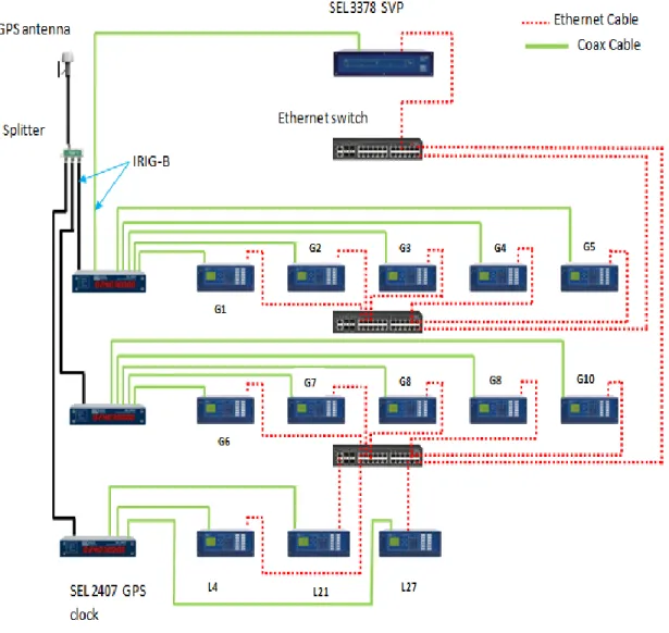
Figure 2.2 shows the phasor system components used in this study. It consists of: SEL 2407 GPS satellite-synchronized clocks, SEL PMUs, SEL 3378 SVP, and secure communications, through an Ethernet Switch.

(26)

16

Figure 2.2 Phasor network diagram

2.5Real Time Simulation

The real time digital simulator used in this study is an eMEGAsim OP5600 HILBox, developed by OPAL-RT Technologies. The eMEGAsim Real-Time Digital Simulator integrates the OPAL-RT powerful electrical circuit solvers, SimPower System, and RT-LAB distributed processing software, and hardware platform for high speed and real-time simulation of electromagnetic transients (OPAL-RT).

(27)

17

Real time simulation has the power to simulate everything from fast electromagnetic phenomenon to the transient stability of large power systems. Therefore, operation of the protection devices in critical system conditions could be tested using this technology.

2.5.1 Software Requirements

The software component of the eMEGAsim is RT Lab, designed by OPAL-RT Technologies, which allows the user to perform real time simulation such as HIL tests. RT Lab is fully integrated with the Matlab Simulink. The software is installed in a host computer which is connected to the target, simulator hardware, through the Ethernet cable. RT-Lab allows the user to create and compile the model by generating C code, load the model into different processor cores, and execute the model in real time.

2.5.2 Hardware Requirements

The hardware component of the eMEGAsim is the OP5600 Chassis. The target computer included in the OP5600 Chassis consists of the following components (OPAL-RT):

• ATX motherboard, with up to 12 processor cores • 6 DRAM connectors

• 250 GB hard disk • 600 W power supply

• PCIe boards, up to 8 slots, depending on the configuration

(28)

18

2.5.3 RT Lab Software

To create a model for real time simulation in RT lab, it is required first to create the model in Matlab Simulink and perform load flow and machine initialization. Then run it offline using trapezoidal solver. If there are any problems in the execution of the simulation in the offline mode i.e. non real time, it is better to be solved earlier in the Simulink. When the model is error free, RT lab component such as artimes and OPcomm blocks should be added to the model, and the solver method should be set to art5 (Solver developed by OPAL-RT) for real time simulation. Also before running in real time mode, transmission lines model should be changed from regular Simpower system (SPS) blocks to artimes Distributed Parameters Line (DPL) blocks.

To allow the execution of the model by parallel processing, the model should be regrouped into subsystems. Each RT lab model should have 0 or 1 console subsystem, 1 master subsystem and any number of slave subsystems depending on the number of processors available.

RT lab provides user interface and interactive environment by allowing monitoring and controlling the model under real time simulation through the console subsystem. The console subsystem contains user interface blocks, such as scopes and controls. On the other hand, the slave subsystem contains all the computational elements of the model, such as generators, transmission lines, transformers and loads. In addition to that, it contains the mathematical operations and input/output (I/O) blocks. The number of slave subsystems could be zero or more per model depending of the grid size.

When the model is large, simulating the model in real time using only one core in the target is not possible. In this case, the model should be divided into multiple subsystems to

(29)

19

distribute the computational elements across multiple cores. In this study, the model is divided into four slave subsystems to allow modeling in real time without having overruns.

To simulate the overhead transmission line, DPL block is used. However, it is necessary to set the simulation time step less than the shortest propagation time of the transmission line in the model. The shortest line in the model is line 5-6 which has a 47.5 µsec propagation time. Therefore, the time step required for the simulation should be less than 47.5 µsec, and consequently, time step of 40 µsec has been selected for modeling IEEE39-bus system in real time.

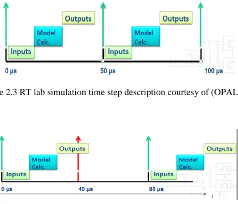
To perform real time simulation, the fixed time step solver should be used, and the simulation type should be discrete. Fixed-step solvers solve the model at regular time intervals from the beginning to the end of the simulation (OPAL-RT). In each time step the simulator performs all necessary calculations to simulate the model. Figure 2.3 clearly describes the concept of discrete time step. This fixed amount of time is called step size. When a predetermined time step is too short and could not have enough time to perform inputs, model calculation and outputs, there is an overrun (OPAL-RT). When an overrun occurs, one time step will be omitted. The next computation will be performed at the next time step. Figure 2.4 shows how overruns cause time step skipping.

RT Lab assigns one processor per subsystem. The processor has a limited capability, depending on the type of blocks used (i.e. require switching operation modelling or not) and the number of blocks in the subsystem. RT Lab allows the user to see the percentage usage of the processor in real time. If the percentage usage is high, there is a risk of the getting inappropriate signal or overruns.

(30)

20

Figure 2.3 RT lab simulation time step description courtesy of (OPAL-RT)

Figure 2.4 Overruns in real time simulation courtesy of (OPAL-RT)

When overrun occurs, it causes data loss by skipping a time step. Therefore, the model is no longer running in real time. To avoid overruns, the IEEE39-bus system model is divided into four subsystems. It is necessary to monitor the model execution in real time before starting the actual testing to make sure there are no overruns.

2.6Hardware in the Loop Test (HIL)

Testing new devices or protection schemes in the real power grid is unattainable, although testing is required before putting the new scheme for operation. Hardware in the loop (HIL) test allows testing actual devices by simulating the power systems in real time with time step less than or equal to 50 µsec for power grids. It allows the interaction between the device under test and the power system simulated through input/output interface boards. Also it

(31)

21

provides user interface which allows the user to monitor or even control the plant in the simulator through performing control actions in real time.

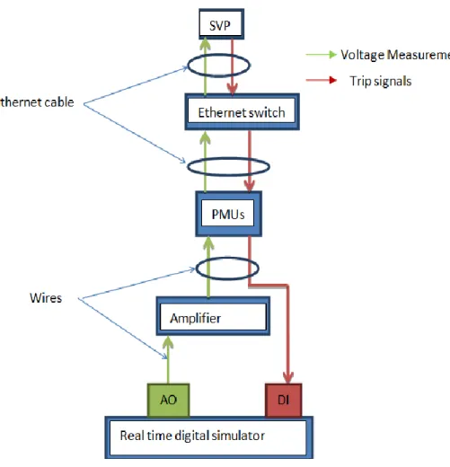
HIL testing platform used in this study is shown in figure 2.5. It clearly shows the plant under simulation, IEEE39-bus system, being loaded into simulator, and the connection between the actual devices under test and the simulator. For simplicity, only one PMU is shown. Figure 2.6 shows a general description of the implementation, as shown the PMUs continuously measure the voltages outputted from the analog output port (AO) of the simulator. The PMUs send these measurements in real time to the SVP via Ethernet cable. If load shedding trip signal is required, the SVP sends a remote bit via Ethernet cable to the associated relay which in turns asserts associated output contact. The output contact is wired directly to the digital input (DI) port of the simulator. The DI input port converts the signal to a logical signal inside the Matlab model to open the associated circuit breaker feeder.

(32)

22

(33)

23 CHAPTER 3 METHODOLOGY

3.1IEEE 39-Bus System Model

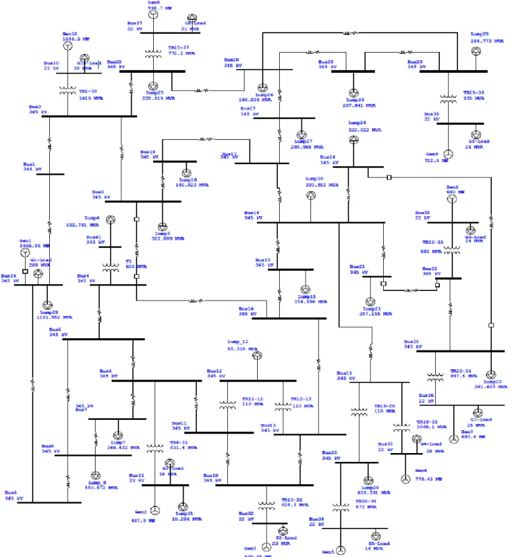
The New England 39-bus system consists of 10 generators, 34 transmission lines, 12 transformers and 18 load buses as shown on Figure 3.1. The swing bus, bus 31, is connected to generator number 2. All other buses which have a generator connected to them are considered as a PV or voltage control bus. The load buses are considered as PQ bus for load flow. For complete system data see appendix (A).

(34)

24

(35)

25

The base voltage for the transmission system is 345kV (L-L) and 22KV (L-L) for the generators, except bus 39 which is connected directly to the transmission system. The IEEE39-bus system is similar to a large power grid in terms of power capacity, system voltages level, and number of buses, lines, transformers and generators.

In order to eliminate having numerical oscillation when a disturbance, such as generator outage, is introduced in the model, a snubber circuit consisting only of resistance is connected in parallel with each generator. The value of the resistance depends on the time step used to perform real time simulation. For example, a model running with a 50 µsec time step, should have a resistance with value of 5% of the machine rating. Since the IEEE39-bus system is modeled with 40 µsec time step, a resistance with value equal to 4% of the machine rating should be connected in parallel with each generator. The swing bus should compensate for these additional resistances.

The eMEGAsim real time digital simulator has 12 core processors. Only 6 of them are licensed and available for use, therefore, in order to simulate the model without having overruns, the IEEE39-bus system is divided into four slave subsystems: southwest, southeast, northwest and northeast subsystems as shown in figure 3.2. Each subsystem constitutes an area which has its own generation and loads. The four subsystems are connected by tie-lines.

(36)

26

Figure 3.2 IEEE39-bus system RT Lab model

Each one of these subsystem was assigned to one processor for the execution of model in real time, and additional processor was assigned to the console subsystem. Figure 3.3 clearly shows subsystems assignation by RT Lab. As shown, RT Lab assigns one processor for each subsystem. Furthermore, to enhance the performance of real time simulation, eXtreme High

Performance (XHP) mode is enabled. The model is built, loaded and ran in the eMEGAsim real time simulator with zero overruns.

(37)

27

Figure 3.3 RT Lab assignations of processors

The four subsystems and their purposes are as follows: 1. Northwest slave subsystem

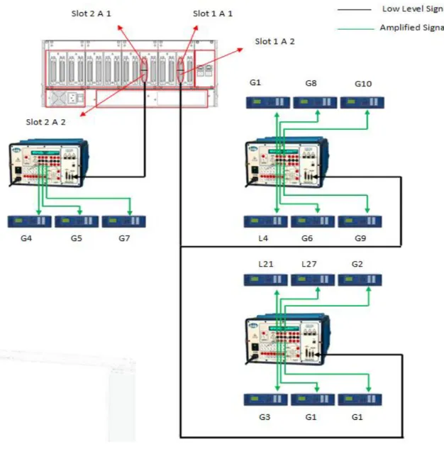
It consists of three generators G1, G8 and G10 in addition to one selected load bus L4. In RT Lab model phase A voltage, from all three generator buses and the load at bus 4, is directed to the slot 1 A subsection 1 in the analog output port in the simulator. The associated output channels of these 4 voltage signals are wired to Doble amplifier then to the associated VT terminals in the actual relays. Moreover, all these signals are recorded using OPwrite block from RT Lab and saved into a Matlab file for further analysis.

2. Northeast slave subsystem

It consists of two generators G6 and G9 in addition to two selected load buses L21 and L27. In RT Lab model phase A voltage, from the two generator buses and the load buses, is

(38)

28

directed to slot 1A subsection 2. The associated output channels of these voltage signals are wired to Doble amplifier then to the associated VT terminals in the actual relays. Furthermore, all these signals are recorded using OPwrite block from RT Lab and saved into a Matlab file for further analysis.

3. Southwest slave subsystem

It consists of two generators G2 and G3. No load buses were selected in this subsystem. In RT Lab model phase A voltage, from the two generator buses, is directed to slot 2A subsection 1. The associated output channels of these voltage signals are wired to Doble amplifier then to the associated VT terminals in the actual relays. Moreover, all these signals are recorded using OPwrite block from RT Lab and saved into a Matlab file for further analysis.

4. Southeast slave subsystem

It consists of three generators G4, G5 and G7. Also no load buses were selected in this subsystem. In RT Lab model phase A voltage, from all three generator buses, is directed to slot 2A subsection 2. The associated output channels of these 4 voltage signals are wired to Doble amplifier then to the associated VT terminals in the actual relays. Also all these signals are recorded using OPwrite block from RT Lab and saved into a Matlab file for further analysis.

On the other hand, the console subsystem provides an interactive environment by providing a user interface. It gives the user the complete monitoring of the system while the simulation is running in real time. As shown in figure 3.4 the OPcomm block collects the signals from the slave subsystems, and then a demultiplexer is used to separate the generators signals from transmission system voltages. When the simulation is running in real time, the user can monitor the status of the system by opening the scope window. The console is programmed to

(39)

29

give the user the capability of controlling the switching devices, such as a generator circuit breaker, applying a fault, and enabling/disabling the recording of the data in real time.

(40)

30

From each slave subsystem the required analog signals are directed to the output ports of the OP5600 HILBox simulator. These signals are phase A voltage from all the generators as well as selected load buses. The voltage signals from the generating station is required to calculate the frequency at the Centre of inertia (COI) and to compute the disturbance power based on the rate of change of frequency of generators.

The IEEE 39-bus system model was built successfully using Matlab Simulink and then imported every time by OPAL-RT RT Lab software for real time simulation. The system is simulated in real-time using eMEGAsim Real-Time Digital Simulator with zero overruns.

3.2Equipment for the Implementation

1. eMEGAsim Real-Time Digital Simulator OP5600 HILBox OPAL-RT System. 2. Three F6350 Doble Amplifiers.

3. Three SEL-2407 GPS clocks.

4. Seven SEL-487E relays used as PMUs. 5. Six SEL-411L relays used as PMUs. 6. SEL-3387 SVP.

7. Three Ethernet switches used to connect all devices in one LAN.

3.3Software for the Implementation 1. RT lab and Matlab Simulink.

2. SEL-5030 ACSELERATOR QuickSet® software.

3. SVP configurator.

(41)

31 5. F6 Doble control configurator.

3.4Amplifiers

Since the OP5600 HILBox real time digital simulator generates a maximum of 16V in the analog output port, and the relay nominal voltage is rated at 66.39 V, line to ground voltage, an amplifier is required to amplify the voltage signals to the relay voltage levels.

In the Matlab model the transmission voltage level is set to 345kv (L-L) and 22kv (L-L) for the generators. These values are virtual values to be used in the simulation. However, to perform HIL test, the simulator should send these signals to the analog output port, and before sending them a gain block should be inserted to bring these high voltage levels down to the simulator I/O port voltage limit.

In RT lab a gain value of 5.931/199185 is used to get a 5.93 V at the simulator output port for the load buses. However, for the generator buses, a gain value of 5.931/11500 is used to get a 5.93 V at the simulator output port. To raise the low level voltage signals at the simulator analog output port to the relay secondary rated voltage level Doble amplifiers with amplification ratio of 6.7/75 are used.

In order to configure the amplifier, F6 Multiple Amplifier Configurator software was used. The software is installed in one computer. All amplifiers along with the computer were connected in one Ethernet network to help making the configuration process of each amplifier flexible and easy.

F6350 amplifiers have the capability of amplifying both low level voltage and current signals, using different and multiple amplification ratios, for both voltage and current. It has the capability to amplify up to 6 low level voltage as well as current signals. In this study, only

(42)

32

voltage sources channels were used, consequently, the amplifiers were configured to amplify only low level voltages. Therefore, six voltages and currents (6V & 6I) sources in the F6 Multiple Amplifier Configurator software are chosen with current sources set to off.

(43)

33 3.5SEL-487E and 411L Relays

State of the art protective relays from Schweitzer engineering laboratories (SEL) which have the built in PMU functionality are used in this study. The relays used are SEL 487E Station Phasor Measurement Unit and 411L Protection Automation Control. The words relay and PMU are used interchangeably throughout this study.

Since SEL PMUs are usually incorporated as a function in a multifunction microprocessor protective relay, all the protection elements such as overcurrent, distance and differential, in the SEL relays were disabled and only PMU function was activated. A setting file which includes the required setting for the PMU function was created for each PMU using SEL SEL-5030 ACSELERATOR QuickSet® software.

In this study, the relays were connected in local area network (LAN), and SEL-5030 ACSELERATOR QuickSet® software is installed in one PC. The PC was used to send/read the setting file to/from the relays. However, for documentation purposes, in each station a database containing the setting files for the relays was created. This provides flexibility and easiness for setting changes.

One significant advantage of the PMU is that it has the capability to calculate the rate of change of frequency of the analog signal and send it to upper control center. The SEL-487E and SEL411L automatically includes the frequency and rate-of-change-of frequency in the synchrophasors messages.

In this study, a total number of 13 PMUs were used. Therefore, to provide a GPS signal for all PMUs, two SEL-2407 and SEL-2401 GPS clocks were used. Each clock provides up to 6 channels, IRIG-B, outputs which provide reference signals for six PMUs. Additionally, the SVP

(44)

34

itself has the capability of providing one IRIG-B output signal which could be used as an IRIG-B input for one PMU.

3.5.1 PMU Function Setting 3.5.1.1Global Setting

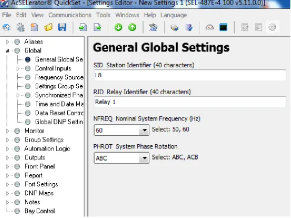
General system properties, such as nominal frequency and phase rotation, was set along with station as well as relay identifier. The nominal frequency is very important for PMU application because PMU sampling and message rate depends on the nominal frequency of the system. Figure 3.6 shows the general setting for the PMU used for PMU located at bus L8.

(45)

35

However, it is necessary to enable the PMU functionality in the PMU setting file first in order for the relay to operate as a PMU. If PMU functionality is disabled, the SEL 5030 SEL-5030 ACSELERATOR QuickSet® software does not allow setting of the other PMU parameters. For synchrophasor protocol setting, IEEE C37.118 message format is used for all PMUs.

For the PMU application a fast response, F, setting is used. This means that the relay uses a high frequency digital filter to filter the measurement samples. The number of phasor data configurations was set to two, the first PMU is used to send the phasors to SVP, and the second one is used to send phasor measurements to Synchrowave central admin software for visualization purposes and comparison of the results.

Determining PMU frequency application setting is required because the rate of change of frequency calculation is dependent on it. Therefore, for PMU frequency application a setting of S used for smooth frequency application in which 9 cycles of data used for the rate of change of frequency calculation.

Frequency-Based Phasor Compensation (PHCOMP) is enabled, which activates the algorithm that compensates for the magnitude and angle errors of synchrophasors for frequencies that are off nominal (SEL-Inc, 2012). All PMUs were set to send only positive sequence voltage in the phasor data set. General settings for the PMUs are shown in figure 3.7.

(46)

36

Figure 3.7 PMU general setting

In the phasor data configuration setting, unique station name was used for each PMU. Additionally, each PMU should have a unique hardware identifier ID, and this identifier in the PMU setting file and in the SVP configuration setting should match each other. Figure 3.8 shows a setting parameters used for phasor data configuration utilized in this study.

(47)

37

Figure 3.8 Phasor data configuration

3.5.1.2Communication Port Setting

For PMUs located in the load buses user datagram protocol (UDP_T) transport scheme was used. This allows the PMU to send synchrophasor packets to the SVP as well as receiving remote bit from the SVP using the same transport channel. This is required because the SVP can only send the control commands using UDP_T or UDP_S transport schemes. On the other hand, the PMUs located at the generator buses, were set to use transmission control protocol (TCP) transport scheme. As each PMU has a unique PMU ID, port number, and IP address, the SVP assigns each PMU measurements accordingly. Figure 3.9 shows communication port setting for load bus PMU.

(48)

38

(49)

39 3.6SVP Program

In this implementation, the SVP represents the central processing unit and contains the load shedding algorithms. The SVP Configurator software is used to connect to the SVP hardware, and it is used also to load and run the program in the SVP. The SVP is programmed to collect the measurements from all PMUs, time aligns these measurements and uses them to assess the system frequency.

3.6.1 Adaptive UFLS Main Program

The adaptive UFLS program is written in the SVP using IEC 6113-3 programmable logic controller standard language. When the simulation is running, the program starts recording the healthy voltages of the load buses, and continuously calculates the COI frequency.

The frequency from each generator is required to calculate the frequency at the center of inertia COI. At normal operating conditions this should be equal to system frequency. When there is a disturbance condition, such as generator outage, the COI should be recalculated with the generator taken out is excluded.

The COI for the IEEE39-bus system is continuously calculated in real time in the SVP, using the frequencies sent by the PMUs located in the generator buses. In this study, the disturbance which causes underfrequency condition was selected to be generator outage. Thus, when one generator tripped off, the rest of the system generators try to share the disturbance power between them depending on their rating, inertia and location from the disturbance area.

When the disturbance is introduced, the COI frequency starts to decline. Therefore, the COI is used in the SVP program as triggering criteria to enable the recording of the generators

(50)

40

rate of change of frequency as well as the load bus voltages at the disturbance moment. Simply, this is achieved by comparing the COI to a frequency of 59.95 Hz as shown in figure 3.10.

Figure 3.10 COI frequency calculation in the SVP program

When the disturbance is initiated, the rate of change of frequency for each generator is recorded for one second. This valuable information is used to compute the disturbance power for each generator, and by adding them the total disturbance power is obtained.

When the COI frequency is less than 59.95 Hz, recording is enabled.

(51)

41

After the disturbance power is computed, the SVP distributes the disturbance power among the load buses. The algorithm uses the voltage dip information from the load buses to distribute the shed power between them adaptively i.e. the load bus near the disturbance should share the larger amount of power to be shed. This is performed by ranking the load buses based on their voltage dip. The load bus with higher voltage dip shares the larger amount of power to be shed.

The voltages of the load buses before disturbance were recorded in matrix to be used later for voltage dip calculation. When the disturbance is initiated by opening the generator circuit breaker, the recording of the voltages at the disturbance is enabled, and at the same time, the recording of the normal voltages is disabled. The average for the healthy voltages as well as voltages after the disturbance is calculated for each load bus. Finally, a voltage dip for each load bus is calculated using equation (2.5).

After the computation of the amount of power to be shed, and its distribution among the load buses is completed, an actual trip signal should be sent. Firstly, from the SVP to the load bus’s PMU over the Ethernet if load shedding is issued to it, and secondly, from the PMU output contact to the associated digital input of the OPAL-RT eMEGAsim real time digital simulator. Then, the signal is directed to the specified load bus circuit breaker feeder in order to open the circuit breaker and shed the load from the bus.

Each load block is assumed to be divided to a number of feeders, each one of them has its own circuit breaker. The number of feeders, and consequently circuit breakers should be kept as minimum as possible because RT Lab software requires a maximum of 12 switches per one subsystem. Therefore, it is necessary to have small number of switches in the model to avoid overruns when simulating in real time.

(52)

42

The output contacts: OUT201, OUT202, and OUT203 in the PMU setting file for each load bus, was programmed to receive three remote bits RB01, RB02 and RB03 respectively. Each remote bit is assigned to one circuit breaker feeder.

When the SVP activates the remote bit(s), the associated output contact(s) is/are closed, the output contact(s) is/are wired to the digital input port of the OPAL-RT real time digital simulator, and once the digital input signal(s) is/are activated the associated circuit breaker(s) is/are opened to shed the load. In order to clear the remote bit after load shedding is achieved, a fast operate clear function should be used.

3.7Station Setup and Local Area Network

Since the Smart Grid and protection laboratory is equipped with state of the art equipment, a Local Area Network (LAN) was established to connect all the intelligent electronic devices (IEDs) used in one network using Ethernet switches. The purpose of this is to emulate the actual modern substation environment. All equipment in the lab OPAL-RT eMEGAsim real time digital simulators, desk top PCs, Doble Amplifiers, SEL PMUs and SEL 3378 SVP, have the capability of communication through Ethernet.

The total number of PMUs used in this study was 13 PMUs. There were 10 PMUs located at generators buses, and these were required to send phasor voltage and rate of change of frequency in real time from each generator in the system. On the other hand, due to availability of limited number of PMUs, only three candidate load buses were considered for the load shedding, and hence, three PMUs were located at load bus 4, 21, and 27.

The actual station layout consists of three stations, station 1 which contains five generator’s PMUs, G1, G2, G3, G8 and G10 in addition to two load buses PMUs, L4 and L27.

(53)

43

This station is equipped with 2 Doble Amplifiers which give 12 analog voltage signals. The eMEGAsim real time simulator is installed in this station.

Station 2 contains three generators PMUs, G4, G5 and G7 in addition to one load bus PMU L21. On the other hand, station 3 contains two generators PMUs, G6 and G9. This station is equipped with one Doble Amplifier which is used also for PMUs in station 2. The three stations were connected in one LAN network.

(54)

44 CHAPTER 4

RESULTS AND DISCUSSION

4.1Adaptive UFLS Results

Different disturbance scenarios were applied in order to test the adaptive UFLS algorithm. To create the underfrequency disturbance conditions, only one generator was tripped off each time. A brief description of each generator outage case is given in the following sections.

Before running real time simulation, load flow and machine initialization were performed using Matlab Simulink. The model was built, loaded and ran successfully in OP5600HILBox real time simulator with zero overruns.

As mentioned earlier in section 3.1, the console subsystem allows performing control actions, such as tripping off generators or applying faults on the model while the simulation is running in real time. Each generator in the IEEE39-bus system has a circuit breaker, the control for this circuit breaker is accessible through console subsystem in the RT Lab software. The generator outage was performed in real time, while the simulation was running through the opening of the generator circuit breaker from the console subsystem.

In order to capture the pre-disturbance and post disturbance values for the frequency, rate of change of frequency, and voltages of the load buses, the writing to Matlab file process should be enabled before opening the generator circuit breaker. The disturbance power is then computed in Matlab using the rate of change of frequency data.

(55)

45

Each time load shedding was required, the SVP sent remote bits over the Ethernet to the selected load bus(es) relay, and accordingly the relay closed the associated output contact(s). when the contact(s) closed, the associated digital input pin(s) of the simulator is/are activated. Finally, the RT lab software directed the signal(s) at the digital input port to the associated feeder circuit breaker in the model, and consequently, the load was shed in real time to bring the system frequency back to a stable level.

Three generators were selected to be taken out. Therefore, three test cases were performed. In each case a generator outage is performed in real time. The SVP operation, PMUs, output contacts status, and simulator digital input port pins status were monitored, and the results were obtained for each case. Furthermore, for each case the amount of disturbance power calculated by Matlab and SVP was obtained, also the relay event files were retrieved for post disturbance analysis.

4.1.1 Test Case 1: Generator 5 Outage

Generator 5 was tripped off in real time, by opening its circuit breaker from the console subsystem. Directly after opening the breaker, the power generated from G5 dropped to zero and its speed increased above 1 P.U. From load flow results, G5 generates 508 MW during normal operating conditions before the disturbance.

Also directly after G5 outage instant, the COI frequency decreased. Therefore, the recording of disturbance power from each generator as well as voltages in the load buses after disturbance is enabled in the SVP program.

(56)

46

For each generator the rate of change of frequency is recorded by RT Lab using OpWrite block as shown in figure 4.1. The file is saved as a Matlab file and imported after real time simulation is stopped for post disturbance analysis.

Figure 4.1 Rate of change of frequency recording in RT Lab

Using equation (2.2) the total disturbance power was calculated and plotted by Matlab. Figure 4.2 shows the total disturbance power when G5 was lost. As shown the total disturbance power, initially after the disturbance, calculated by Matlab was 314 MW.

(57)

47

Figure 4.2 Total disturbance power recorded in Matlab for case 1

On the other hand, the SVP estimated the total disturbance power using equation (2.2) to be 312 MW as shown in figure 4.3

Figure 4.3 Total disturbance power estimated by the SVP for case 1

69.4 69.45 69.5 69.55 69.6 -300 -250 -200 -150 -100 -50 0 X: 69.4 Y: -314.1 Time (sec) D is tu rb a n c e P o w e r (M W )

(58)

48

Figure 4.4 shows voltage dip as well as shed power, for load buses, recorded by the SVP program when G5 was tripped off. In this case, load bus 21 had the highest voltage dip. Therefore, it shared the largest amount of power to be shed, and this is because it is located near the disturbance location.

Figure 4.4 Voltage dip and shed power for each load bus recorded by the SVP for case 1

(59)

49

Based on the voltage dips recorded, the SVP shed the load as shown in table 4.1.

Table 4.1 Adaptive UFLS Results for Case 1

Bus 4 Bus 21 Bus 27

V dip % MW shed V dip % MW shed V dip % MW shed 1.3 86 1.88 123 1.57 103

When G5 was tripped off, the system frequency dropped to less than 57.4 Hz when no load shedding was applied as shown in figure 4.5.

Figure 4.5 Frequency response without load shedding for case 1

120 140 160 180 200 220 240 260 57 57.5 58 58.5 59 59.5 60 60.5 Time (sec) F re q u e n c y ( H z )

(60)

50

On the other hand, when adaptive UFLS was applied, the SVP started to shed the load instantaneously when the system frequency dropped below 59.5 Hz and consequently, system frequency recovered as shown in figure 4.6.

Figure 4.6 Frequency response with adaptive UFLS for case 1

When conventional UFLS scheme was used to recover system frequency, the frequency response showed a higher overshoot compared to adaptive UFLS as shown in figure 4.7. This is because the amount of power to be shed in this case was higher than what SVP estimated in the adaptive UFLS scheme.

620 640 660 680 700 720 740 760 780 59.3 59.4 59.5 59.6 59.7 59.8 59.9 60 60.1 60.2 60.3 Time (sec) F re q u en cy ( H z)

(61)

51

Figure 4.7 Frequency response with conventional UFLS for case 1

Generator 6 was tripped off in real time, by opening its circuit breaker from console subsystem. Directly, after opening the breaker, the power generated from G6 dropped to zero, and its speed increased above 1 P.U. From the load flow result, G6 generates 750 MW during normal operating conditions before the disturbance.

Similarly, using equation (2.2) the total disturbance power was calculated and plotted by Matlab. Figure 4.8 shows the total disturbance power when G6 was lost. As shown the total disturbance power, initially after the disturbance, calculated by Matlab was 540 MW.

380 400 420 440 460 480 500 520 540 59.4 59.6 59.8 60 60.2 60.4 60.6 60.8 Time (sec) F re q u e n c y ( H z )

(62)

52

97.2 97.3 97.4 97.5 97.6 97.7 97.8 97.9 -500 -400 -300 -200 -100 0 X: 97.45 Y: -539.9 Time (sec) D is tu rb a n c e P o w e r (M W )

(63)

53

Figure 4.10 shows voltage dip as well as shed power, for load buses, recorded by the SVP program when G6 was tripped off. Also in this case, load bus 21 had the highest voltage dip. Therefore, it shared the largest amount of power to be shed, and this is because it is located near the disturbance location.

Based on voltage dips recorded, the SVP shed the load as shown in table 4.2.

Bus 4 Bus 21 Bus 27

V dip % MW shed V dip % MW shed V dip % MW shed 2.7 140 4.9 246 3.4 172

(64)

54

50 100 150 200 55.5 56 56.5 57 57.5 58 58.5 59 59.5 60 Time (sec) F re q u e n c y ( H z )

(65)

55

When conventional UFLS scheme was used, to recover system frequency, the frequency response showed a higher overshoot compared to adaptive UFLS as shown in figure 4.13. This is because the amount of power to be shed in this case was higher than what SVP estimated in the adaptive UFLS scheme.

480 500 520 540 560 580 600 620 59 59.2 59.4 59.6 59.8 60 60.2 60.4 Time (sec) F re q u e n c y ( H z )

(66)

56

Figure 4.13 Frequency response with conventional UFLS for case 2

Generator 8 was tripped off in real time, by opening its circuit breaker from console subsystem. Directly, after opening the breaker, the power generated from G8 dropped to zero, and its speed increased above 1 P.U. From the load flow result, G8 generates 660 MW during normal operating conditions before the disturbance.

Similarly, using equation (2.2) the total disturbance power was calculated and plotted by Matlab. Figure 4.14 shows the total disturbance power when G8 was lost. As shown the total disturbance power, initially after the disturbance, calculated by Matlab was 376 MW.

140 160 180 200 220 240 260 280 300 59 59.5 60 60.5 61 61.5 Time (sec) F re q u e n c y ( H z )

(67)

57

57.1 57.2 57.3 57.4 57.5 57.6 57.7 57.8 -400 -350 -300 -250 -200 -150 -100 -50 0 Time (sec) D is tu rb a n c e P o w e r (M W ) X: 57.51 Y: -376.2

(68)

58

Figure 4.16 shows voltage dip as well as shed power, for load buses, recorded by the SVP program when G8 was tripped off. In this case, load bus 27 had the highest voltage dip. Therefore, it shared the largest amount of power to be shed, and this is because it is located near the disturbance location.

Based on the voltage dip recorded, the SVP shed the load as shown in table 4.3.

Bus 4 Bus 21 Bus 27

V dip % MW shed V dip % MW shed V dip % MW shed 1.8 100 2.3 125 3 168

(69)

59

50 100 150 200 56 56.5 57 57.5 58 58.5 59 59.5 60 Time (sec) F re q u e n c y ( H z )

(70)

60

When conventional UFLS scheme was used to recover system frequency, the frequency response was very simila