Server Provisioning in Content Delivery Clouds

Server Provisioning in Content Delivery Clouds

Abstract—Cloud based video delivery platforms serve a signif-icant fraction of the entire Internet traffic and are continuously expanding with the growing demand. We study the provisioning of the server cluster to deploy at each location in such systems. We optimize the right server count, peering bandwidth, and server configuration as the disk size and the necessary SSD and/or RAM caches to sustain the intensive I/O load. Our analyses are based on actual server traces from a global content delivery platform. Our optimization captures the interaction of cache layers in each server, the interplay between egress/disk capacity and network bandwidth, storage read/write constraints and storage prices.

Keywords-video content delivery network; resource allocation I. INTRODUCTION

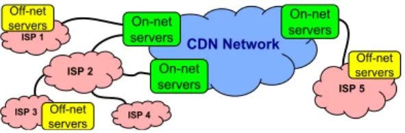
Video streams constitute over half the entire Internet traffic. This substantial volume is usually delivered to users through a large cloud of servers commonly known as a Content Delivery Network (CDN). The generic layout of such platforms is illustrated in Figure 1. It consists of dozens ofon-netserver locations residing in the CDN network such as in its datacenters or peering points [2], [3], as well as a large number of off-net servers located inside ISPs worldwide [1], [4]. For example, Akamai reports their presence in a growing number of currently 1,300 ISPs around the world with 170,000 servers [1],

To keep up with the demand, the content delivery cloud has to be constantly growing. For instance, the Akamai platform has expanded nearly3×in size from 2010 to 2015 [1], [8]. The growth includes adding servers to existing server locations as well as more and more new locations worldwide to maximize edge serving. Proper provisioning of the deployments is a critical task that determines the CDN’s cost and efficiency and is the problem of our interest in this paper.

In an oversimplified view, this problem includes finding the right cache size to achieve a desired caching efficiency at each target location; cache efficiency is similar to and generalizes cache hit rate (cf.§II). The practical problem, however, poses more fundamental challenges. First, the cache efficiency to target is not a given, rather a central parameter to optimize. Due to the power-law pattern of video popularities [9], gaining every few percent of cache efficiency requires exponential increase in cache size. The consequent cost may easily outweigh that of just settling for a lower cache efficiency and letting some costly traffic get past the server. Second, a certain number of deployed servers can egress (serve) up to a certain capacity. Over-provisioned server clusters that rarely get to full utilization are a waste of hardware and space. Smaller deployments, on the other hand, result in more costly traffic getting past the servers which may be reasonable to some extent or not at

On-net servers ISP 1 ISP 4 Off-net servers CDN Network On-net servers On-net servers ISP 2 ISP 3 ISP 5 Off-net servers Off-net servers

Fig. 1. General network model of a global CDN.

all, depending on the location. Third, cache servers need to designate RAM and/or SSD caches above the disks given the excessive I/O, as we analyze. To sustain some expected egress volume and cache efficiency, a non-trivial combination ofcache layersis required in a server to stand the read and write loads. Depending on their r/w bandwidths and prices, cache layers in a server fundamentally change the classic tradeoff between cache size and network bandwidth. In addition, layering affects the behavior of caching algorithms; they may diverge from their expected size-vs-efficiency operating curve for the workload.

We analyze these and other considerations for deploying new CDN servers at a given location and we build the proper optimization framework. Our contributions are as follows. 1) We conduct a detailed analysis, through actual server traces

from a global video CDN, of the effects of layering the caches in a server, such as disks, SSDs and memory. We investigate whether and how the behavior of caches would change in such layered settings. This behavior is the basis of any cache provisioning study.

2) We develop an optimization algorithm for finding the right server count and server configuration (disk drives and the necessary SSD/RAM caches) to deploy in a location and optionally the peering bandwidth to provide. The process carefully captures the interplay between egress/disk capacity and the upstream traffic getting past the servers, the effect of layering on the caching algorithms, and the read/write constraints and the prices of cache storage drives.

3) We analyze the optimal deployment cluster along multiple dimensions and study its relationship with network costs, constraints, storage read/write bandwidths and prices. The remainder of this paper is organized as follows. The considered CDN model is established in Section II. Related work is reviewed in Section III. Section IV analyzes the layering of caches in a server. The server optimization problem is studied in Section V. Section VI presents experimental results.

II. CONTENTDISTRIBUTION ANDSERVERMODEL

Global video delivery clouds deal with an immense volume of traffic at the scale of terabits per second [1]. Such a delivery

goes with certain considerations in today’s Internet, on which our high level system model is based. The primary concern for platforms distributing voluminous traffic is to avoid high traffic handling costs and overload on bottlenecks; in terms of latency, it is often just enough if the user-to-server round-trip time (RTT) is within a reasonable limit. Therefore, to serve the user traffic of an ISP, usuallyonly a fewof the server locations are preferred such as one inside that ISP or one behind a peering link to the ISP; see Figure 1. That is, servers at different locations handle the traffic of different user networks.

Network model. We consider a generic model where the traffic of user networks from different ISPs is assigned to server locations primarily based on the CDN’s traffic assignment criteria such as the above, as well as RTT limits. Then, the servers in each location manage their own cache contents according to the request traffic of the corresponding user network(s). The rationale behind the choice of this model is twofold.First, as discussed, one cannot expect to freely assign user traffic to arbitrary server locations based on, e.g., what individual video ID is requested and which server should host it, as in DHT and cooperative caching for lighter traffic [11], [14], [5]. This would result in, for instance, sending user traffic from one ISP to off-net servers in another (competing) ISP; sending to on-net servers with no peering path to ISP; having servers proxying traffic through those in other ISPs or behind no peering link. Note that the detailed mapping of users to server locations is an orthogonal problem to the current work and our server provisioning study is irrespective of the specific mapping strategy implemented by a CDN. The discussed model is to illustrate our target type of CDNs among (inapplicable) alternatives.Second, for a CDN with thousands of servers and millions to billions of videos, we do not assume the existence of a content tracking database: one that tracks the highly dynamic per-locationpopularity and availability of videos across CDN server locations. This database would be required for (logically) centralized content management across the servers [20], [7]. However, instead the servers in each location manage their own cache contents based on the request traffic they each receive.1

This scalable approach is known as the non-cooperative pull-based model in the literature [19]; the servers can indeed take any arbitrary (non-intrusive) extra measure as well, e.g., exchanging video popularity information in localities [16].

Cache server model. As described, each server maintains a dynamic collection of video pieces that are most popular for the user network(s) it serves. This normally requiresredirecting the requests for video pieces too unpopular to live on the disk (HTTP 302), e.g., to an upstream, larger server location with a proper path to the ISP2_{. This is because caching unpopular}

content pollutes the disk. Also, it can overload the disks with excessive writes: unpopular videos observe only one or very few

1_{A common practice for caching content on a cluster of servers is toshard} the content ID space over co-located servers via a simple hash-mod function or consistent hashing. This is to avoid co-located duplicates and increase the depth of the caches. Thus, one may think of the servers in a location as one large server serving the whole content ID space.

2_{The server can sometimes act as a proxy, but only if its egress is under} utilized and its ingress not constrained. Otherwise, proxying will just use up two servers’ resources rather than simply redirecting to the other server.

accesses during their lifetime in the cache before being replaced with other (possibly unpopular) content. This overflows the disks and harms not only the write-incurring requests but also regular reads for cache-hit requests. We have observed that for every extra write-block operation we lose 1.2–1.3 reads.

To address this and other requirements for a video CDN cache in addition to traditional caching, we use two caching schemes from previous work [17]. We use these schemes in our experiments. Our server optimization framework, on the other hand, is separate from and independent of the caching algorithm plugged in. The schemes used are calledxLRUand Cafe, either of which can run on a server and manage its disk. Upon a request for a video and some arbitrary byte range, the schemes decide whether the request should be served or redirected and which video pieces should be evicted from disk, if any. They divide the files and the disk into smallchunks of fixed size (e.g., 2 MB) to facilitate partial caching. These schemes provide means for managing the inherent tradeoff between the server’s cache-fill and redirected traffic: the less the server redirects requests, the more it admits and the higher the cache churn and the consequent cache-fill traffic—and vice versa. Cafe cache is more efficient and xLRU is simpler.

Metrics.Suppose a server egressingE Mbps of traffic and redirectingRMbps—requests for video pieces it is not willing to host. Thus,D=E+Ris the total demand seen by the server. SupposeIMbps of the served traffic incurs ingress (cache fill). Hence,E−I is served directly from the cache and I+R is the traffic getting past the server. We definecache efficiencyas

(D−R−I)/D= (E−I)/(E+R), i.e., the standard cache hit rate extended to incorporate redirections. We can also define the cache-fill to egress ratio as I/E, which is a metric we use in our framework. To get a numeric sense,I/E is usually between10% to40% in our experiments andR < I.

Dataset.We base our analyses in this paper on actual server traces from a global CDN serving user-generated video content. The data includes anonymized request logs of a few server locations for a two-month period in 2014. Each request entry in this dataset includes a timestamp, video ID (hashed), playback ID and byte range. The dataset includes about half a billion sample requests for over a million distinct videos.

III. RELATEDWORK

Provisioning of CDNs is studied in [13], [18], [6]. The authors of [6] optimize the bandwidth and the streams for each cache, but do not capture the tradeoff between disk and network cost. The authors of [18] consider this tradeoff and jointly optimize cache sizes and the objects placed on them. A similar work in [13] studies where to place the servers jointly with the placement of objects and routing requests to them. Such works are based on a global view of individual objects and per-client interests. These problems are also different from our target. We aim at finding for an existing CDN the right deployment configuration to install at a given location, e.g., new ISPs expressing interest in hosting CDN servers [4].

Sizing individual cache deployments is studied in [15], [13]. For an ideal request stream of Independent Reference Model (IRM), i.e., ignoring temporal locality, the optimal cache size

is estimated analytically in [15]. For more realistic request streams, an analysis is presented based on running the cache replacement algorithm on the stream. This is similar to how we provide part of the input to our optimization. A similar model to [15] is considered in [13]. These works target the sizing of traditional replacement caches. Also, they assume the server as a single-layer cache. In contrast to our work, they are unaware of the necessary layering of caches in an I/O bound video CDN server—how the layers affect each other’s behavior, how they take loads off each other, and how their read/write constraints and prices interplay with other costs.

Previous works [21], [12] also study the characteristics of the miss sequence of a cache, as it is the potential input to another cache. Given the complexity of such theoretical modeling, these works are based on idealized assumptions, most notably the discussed IRM model for the request stream. Moreover, these studies only consider cache replacement, not cache admission and redirections which is a necessity in our case.

IV. LAYEREDCACHES IN ASERVER

Given the multi-Gbps I/O for serving video workload, a servers needs to designate a part of its RAM as memory cache on top of the disks to mitigate their limited read bandwidths— evaluated quantitatively in Section VI. Moreover, flash storage with its declining cost can be an alternative/additional layer of caching to alleviate this problem while also avoiding the high cost of all-RAM caches. In addition, Phase Change Memory (PCM), a recent persistent-memory technology with significant performance gains over flash [10], can be employed either in between RAM and flash or instead of them, as evaluated in Section VI. Thus, to analyze server provisioning it is necessary to analyze the performance of caches in a 2+ layered setting. A. The Mutual Effects of Layered Caches

Layering the caches alters the input pattern to them as shown in Figure 2 and discussed shortly, and it changes their behavior. To understand this change, let us first review the interactions of the layers in a server. The twofold interaction includes the effect of the lowest layer (disk) on the higher layers as well as the effect of each higher layer on the lower ones.

In a traditional stack of replacement caches, the request stream arrives at the layers from top to bottom, each leaving its miss stream for the next. In a video CDN cache, however, some requests are redirected if they are for video chunks too unpopular to live on the server—less popular than the least popular ones stored. The cache algorithm in the lowest layer (disk) makes this decision, since that is the layer that holds the least popular content. Any interior cache can as well perform cache admission for its own layer: whether a missing chunk is to be stored on the layer or it is to be served directly from the lower layer. Though, the analysis in this section shows that plain LRU replacement is the preferred choice for the interior layers. Put together, in the life of a request it is first checked for admission by the disk-layer cache algorithm, e.g., Cafe (§II). If the requested video chunks are too unpopular to be cached on the disk, they are clearly not worth caching on the interior layers either and it does not make sense to

unnecessarily run the request through them. The request is simply redirected. Our analysis shows shortly that this in fact benefits the caching efficiency of the interior layers. Notice that the disk cache admission algorithm sees all requests including those later served by a higher layer and not read from the disk, therefore it will never redirect a request if the data exists on any of the layers. If the request is admitted, it is sent to the highest layer for serving and possibly flows downwards including to the disk cache itself; this time only for possible cache-fill as it is already admitted.

In this system, first, cache admission leaves a fundamentally different input stream to higher layers, compared to a traditional cache stack where the whole request stream simply flows downwards. Second, adding a cache atop an existing one also leaves a changed input pattern to the lower one, as in a standard cache stack. These two effects are shown in Figure 2 for a sample two-layer cache fed with the traces of a real CDN server. The figure plots the popularity curve for the original request stream (labeled “Original input”), the stream of requests admitted by Cafe in the lower layer (“Post redirection”), and the miss stream of the higher layer (“Past higher layer”). The original request stream follows more or less the expected power-law pattern. The stream hitting the top layer, though, misses the tail which is unpopular content redirected by cache admission. The request stream arriving at the lower layer misses the head of the curve as well, which is popular content served at the higher layer. With either of these two effects on the input stream, a caching algorithm may or may no longer yield the same size-vs-efficiency behavior as its standalone version. Knowing this behavior is critical for deciding cache sizes. B. Analysis

We analyze the layering of caches by simulating a server under real workload in several different layering settings. We consider xLRU and Cafe caching schemes for video CDN servers [17] as well as the standard LRU scheme. LRU, most widely used in today’s Web caches, can be employed in the interior layers although it does not support the requirements of our target cache servers. This is because an interior cache is only a protection layer and does not necessarily have to distinguish ingress and redirected traffic. It can also simply operate on the basis of single video chunks without having to make one serve-vs-redirect decision for a multi-chunk range request for chunks of different popularities [17]: LRU can just fetch and cache each single cache-missed chunk from the lower layer. In case of a mixed cache hit and miss for a chunk range request at some interior layer, the original request may be broken into smaller chunk ranges (non-contiguous) when arriving at the lower layer. We let this naturally happen rather than enforcing continuity of requests getting past a layer (assuming this is doable without loss of efficiency); also note that in our traces with 2-MB chunks most requests span very few chunks. We also avoid the complexities of ensuring 100% inclusive cache contents from a layer to the next. As the experiments show next, these complications are not necessary.

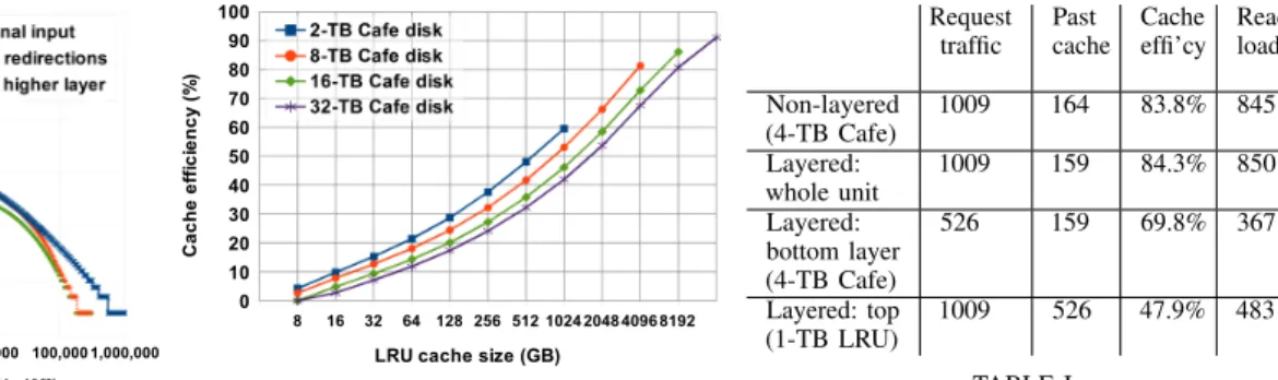
Figure 3 shows the effect of the lowest layer’s admission control on the efficiency of a standard LRU at some higher

1 10 100 1,000 10,000 100,000 1,000,000 1 10 100 1,000 10,000 100,000 1,000,000

Chunk rank (normalized to [1, 1M])

C h u n k h it c o u n t ( n o rm a li z e d t o [ 1 , 1 M ])

Fig. 2. Distribution of requests for video pieces (2-MB chunks) by their rank, a.k.a., thepopularity curve, for a 2-layer cache with a 2-TB Cafe disk and a 256-GB LRU on top. Best viewed in color.

8 16 32 64 128 256 512 1024 2048 4096 8192 0 10 20 30 40 50 60 70 80 90 100

LRU cache size (GB)

C a c h e e ff ic ie n c y ( % )

Fig. 3. The effect of a lower layer Cafe cache on the efficiency curve of a higher layer LRU. The anomaly for 16-TB LRU on a 32-TB Cafe disk is due to the large caches not reaching a fully steady state in the duration of traces.

Request traffic Past cache Cache effi’cy Read load Non-layered (4-TB Cafe) 1009 164 83.8% 845 Layered: whole unit 1009 159 84.3% 850 Layered: bottom layer (4-TB Cafe) 526 159 69.8% 367 Layered: top (1-TB LRU) 1009 526 47.9% 483 TABLE I

THE EFFECT OF ADDING A LAYER ON AN EXISTING CACHE. TRAFFIC NUMBERS ARE INMBPS. “PAST

CACHE”IS THE TOTAL CACHE-FILL AND REDIRECTED TRAFFIC OF THE RESPECTIVE CACHE.

layer. The LRU cache operates on the request stream admitted by the server. Thus, the smaller the disk size (going from one curve to the next), the higher the fraction of videos considered unpopular whose requests are redirected. Consequently, the requests to the LRU cache get more and more exclusive of unpopular content. This yields higher efficiency for the LRU by up to 20%. That is, the efficiency curve of this cache for a fixed workloadcan no longer be estimated on its ownand is a function of the underlying disk cache size and algorithm. This is a key consideration for the server provisioning problem.

To analyze the second effect, the addition of a higher layer cache on an existing one, we evaluate the operation of the three caches, LRU, xLRU and Cafe, on top of each other (9 cases) with different sizes. Our results show that the evaluation of beyond 2 layers is not needed. Table I shows the effect of such layering for a scenario where a 4-TB Cafe cache operates with and without a higher layer 1-TB LRU cache. The efficiency of the 4 TB Cafe cache alone is dropped significantly from 83.8% to 69.8%, given the change in its incoming request traffic; see the capped head in Figure 2. The efficiency of the system as a whole, however, observes marginal change (0.5%). Behind the scenes, the read load on the disk cache is significantly reduced from 1009−164 = 845Mbps to367 Mbps. We expand this comparison to across different cache combinations and cache sizes, which yield similar results to those in Table I and are summarized below. Detailed results can be found in [16].

The findings on layered caches are summarizes as follows.

• A server’s disk cache algorithm and size can significantly

affect the interior layers. The efficiency of a cache as a function of its size, the standard foundation of a provisioning study, cannot be evaluated on its own for the interior layers and depends largely on the disk cache beneath it.

• Adding a layer of smaller size (≤half) on top of an existing

cache, while obviously changing the input to and hiding many requests from it, either does not impact the overall caching behavior of the system or marginally improves it (≤ 2%). This marginal difference only occurs from the lowest layer to the next and not from then on. The new layer takes a significant read load off the lower ones.

• While Cafe and xLRU are the suitable schemes—and Cafe

the most efficient one—for the disk cache, as a higher layer

the standard LRU is the best choice. For yet higher layers above the LRU, the three algorithms make no difference, suggesting the simpler one (LRU) as the preferred candidate.

V. OPTIMIZEDSERVERPROVISIONING

This section presents the server provisioning optimization problem and our solution to it.

The situation for a server deployment differs from location to location. In case of off-net servers, some ISPs may transfer all their upstream traffic through atransitprovider, a.k.a., a parent ISP. Internet transit is often billed by 95%ile bandwidth usage, a measure of peak traffic excluding outliers. Some larger ISPs, on the other hand, may have settlement-freepeeringwith a CDN server location. In this case, upstream traffic towards the CDN may be assumed free up to a certain bandwidth limit. Excess traffic beyond this limit normally makes it way to the CDN server location through an alternative costly transit path. The same situations exist for on-net servers, where their upstream traffic either traverses the CDN’s backbone infrastructure or possibly Internet transit paths: either free, billed by Mbps, or a hybrid. We incorporate these considerations on network cost and its interaction with server configurations.

We consider the problem based on peak-time values. That is, we get peak-time traffic values to meet bandwidth constraints and we assume traffic pricing based on peak-time usage. The problem for the less common case of average-usage pricing can be structured and solved based on the same principles and is not studied separately for space limitation. We also assume that CPU is not a bottleneck tighter than the egress capacity when serving bulky traffic; this is based on our observations from a real-world video CDN. We also assume that the cluster of servers to deploy have the same configuration, for the concern of balanced load. Given content sharding across co-located servers (§ II), the servers receive nearly the same request volume and yield the same caching efficiency and cache I/O. A. Notation

LetI denote the number of cache layers, ci (1≤i≤I) the cost per GB for the storage at layeri where i= 1is the top layer,bi and zi its read and write bandwidth in Mbps, andxi its size to be determined. This size may be provided, e.g., for the disk layer, as one disk drive or a series of them to boost

the r/w bandwidths. We consider an array of same-size disks in the server, which avoids imbalanced hit rates and loads across disks. The number of drives is ki, the size of eachxi/ki, and the aggregated read (/write) bandwidth kibi (/kizi).

Letei,I(xi,xI)be the expected caching efficiency of layer

i when given a size ofxi and the admission controller in the lowest layer is given a size ofxI; see Figure 3. Letfi,I(xi,xI) be the corresponding cache-fill-to-egress ratio (§II). We define

f0,I(·) := 0 and fI(xI) :=fI,I(xI,xI) for convenience. As analyzed, caching efficiency and its breakdown to cache-fill and redirection can be assumed irrespective of higher layers. That is, fi,I(xi,xI) is the fill-to-egress ratio of layers 1 through

i as a whole as long as the layers are of reasonable relative sizes (xj≤xj+1/2). Out of someE Mbps volume of traffic egressed by the server, E(1−fi,I(xi,xI))will get past the caches at layers1throughiand hit layeri+ 1; also recall that the interior layers had better use a plain replacement cache such as LRU (§IV). Upstream traffic is free up to bandwidth limit B Mbps (possible peering/infrastructure), beyond which it incurs a costCper Mbps.Bmay as well be0.Dmaxdenotes the total demand of the corresponding user networks during its peak times. The servers would usually get to full utilization during this time and we can assume y≤Dmax.3

The egress capacity of one server is E (e.g., 4 Gbps), and the total egress capacity to be determined for deployment isy, i.e., the number of servers is y/E. It is indeed not realistic to optimizeyto any arbitrary value, as analyzed shortly. Providing this capacity incurs a cost of w$/Mbps: the cost of a server divided by E. The cost of a server can include the hardware cost of a server (excluding the cache layers) and the possible hosting premium the CDN may need to pay the hosting ISP or Internet Exchange Point, if non-zero.

B. Problem Formulation

The server provisioning problem is formulated as follows. Target variables to be found are bold faced: y,xi andki.

min wy+ y E I X i=1 cixi+ max n y×fI(xI) + (Dmax−y)−B,0 o ×C (+P×B) (1) s.t. E×fi,I(xi,xI)≤kizi(1−ǫ) (2) E×(1−fi,I(xi,xI))− E×(1−fi−1,I(xi−1,xI))≤kibi(1−ǫ) (3) 1 kizi E fi,I(xi,xI) + 1 kibi E fi−1,I(xi−1,xI)−fi,I(xi,xI) ≤ 1 (4) y≤Dmax ; xi≤xi+1/2. (5)

The objective function in Eq. (1) includes the cost of egress hardware and/or hosting premium (wy), cache storage at each

3_{A cluster not fully utilized even during peak hours would be a waste of} hardware/space that neither the CDN prefers to deploy nor the ISP to host.

layer, and the upstream traffic. This traffic includes the cache-fill and redirected traffic getting past the servers as well as any peak-time demand beyond the egress capacity. When egressing at capacity, the cache-fill traffic of the servers isyfI(xI)and the total of redirected and excess traffic is Dmax−y. This traffic is free up toB Mbps and incurs a cost ofC per Mbps after that. One may consider peering not entirely free since it needs provisioning and incurs cost, while one may take it as an orthogonal cost that will be there in any case. Eq. (1) including/excluding the shaded term (P×B) assumes the former/latter case; in the latter case,Bis a target variable rather than an input constant andP is the unit cost for provisioning peering bandwidth. We analyze both cases in our experiments. Moreover, we can introduce a marginal cost to Eq. (1) for employing smaller storage units, such as 1-TB disk drives rather than 4-TB, which we defer to Section VI.

The constraint in Eq. (2) ensures that we do not overflow the layer-icache of a server with excessive writes under peak load, i.e., when egressing atE Mbps hence incurring a write load of

E×fi,I(xi,xI). A(1−ǫ) factor of the maximum write/read bandwidth (kizi/kibi) is enforced in Eqs. (2) and (3) to ensure a minimum read and a minimum write bandwidth atall times.4

Eq. (3) ensures that the read load (excluding writes) stays within limit. This load equals the total cache reads at layers

1 through i minus those at layers 1 through i−1. We can assume from Section IV that the cache hit traffic of layers

1 through i equals what layer i alone would have achieved which is E×(1−fi,I(xi,xI)). From this load, the cache hit volume of layers1 through i−1 is taken off. We also note that the aggregate r/w bandwidth is more limited than simply

bi+zi, e.g., a disk being read at full bandwidth cannot write data and vice versa. Thus, in addition to the r/w bandwidth limits, we add the constraint in Eq. (4) where the sum of the write and read bandwidth utilizations cannot exceed 1. Eq. (5) includes our original assumptions for reasonable provisioning. C. Optimization Solution

The formulated optimization problem has a rather complex form to be dealt with by standard linear/convex optimization libraries. However, we note the small number of optimization variables (y,xi,ki) and the fact that an exact solution with arbitrary values for them is not going to be helpful anyway. The following make the problem tractable.

• Caches of RAM, disk or other storages can only exist at

certain coarse-grained sizes, e.g., 1 TB disks. The egress capacity is limited in resolution by one server, e.g., 4 Gbps.

• There exist no more than a few layers (I).

• Not any arbitrary combination of possible cache size and

egress capacity values is valid, e.g., a disk of 1 TB does not match an egress capacity of 10 Gbps (by server count). These restrictions on the solution space simplify the opti-mization problem: it can be solved by iterating over the solution space as we have easily done in our experiments. An example

4_{This is to avoid the potential overload in the two extreme ends of the r/w} spectrum, e.g.,ǫ= 0.05ensures that even if the model expects very small write loads for some scenarios we still bound read utilization to a maximum of 95% and always reserve a minimum 5% for writes.

is as follows. There exist up to 4 cache layers and the lowest is disk. We are to deployN servers at the target location, i.e.,

y=NE. Suppose each server can egress up toE= 4Gbps of traffic. Also, a server can hold up to 8 disks of {1,2,4} TB, giving the possible disk caches as {1,2,4} × {1, . . . ,8}— 24 possible values for (x4,k4). Assuming about the same range of variability for the other 3 layers, only 244_≃330

K different combinations exist for each value ofN. In case of joint server and peering bandwidth provisioning discussed earlier, an additional dimension of the possible peering bandwidths (B) is added to the solution space with a similarly small number of values, e.g, by 100 Mbps–1Gbps grains. The optimization has been solved in sub-second time in all our experiments.

Optimization output. In our solution process, we first fix the value of N (equivalently,y) and then optimize {xi,ki} values. In practice, CDN operators benefit more from such listed solutions that maps each Nvalue to a vector {xi,ki} than from a fixed optimal value for all variables including forN. This is specifically the case with off-net deployments. The listed solution, besides being a superset of the singular one, allows more informed decisions between a CDN and ISPs. In practice, the target number of off-net servers to deploy is not only a function of the corresponding hardware and bandwidth costs, but also largely a matter of each ISP’s willingness and ability to provide space for them. An ISP may either host any decided number of CDN servers on a settlement-free agreement (a mutual win), offer to host only a limited number, or charge the CDN a premium for hosting the servers—reflected in parameter

w. In any case, the quantitative figure provided by the optimizer on the resultant hardware and bandwidth cost for each given number of servers (N) is necessary for accurate and informed agreements between the CDN and each ISP.

VI. EXPERIMENTALRESULTS

We analyze the optimal configuration to deploy across a variety of scenarios and examine its relationship with different costs and constraints. As elaborated in Sections II and III, we are not aware of any previous work able to address the requirements of our studied provisioning task.

A. Parameters and Setup

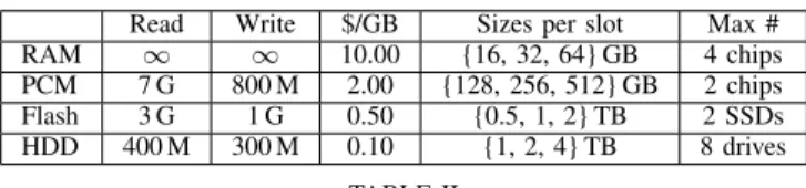
The default values we consider for storage r/w bandwidths and prices are listed in Table II and are varied in a wider range in some experiments. Detailed explanation and data sources can be found in the extended version [16]. Bandwidths in the table correspond to random r/w, not sequential. If having multiple drives, their bandwidths add up. If multiple bandwidth/price configurations exist from different vendors, the optimization can be solved separately for each—each runs in sub-second time. In our experiments, we also make a minor modification to the objective function in Eq. (1) to prefer an obtained cache size (xi) as larger storage drives if all else is more or less the same. For example, assuming the ~0.10 $/GB cost for disk in Table II corresponds to its largest units (4 TB in here), we add10% to the disk cost if 2-TB disks are used and another

10%for 1-TB disks. The corresponding modification to Eq. (1) is trivial and is omitted for clarity. Note also that cost C per

Read Write $/GB Sizes per slot Max # RAM ∞ ∞ 10.00 {16, 32, 64} GB 4 chips

PCM 7 G 800 M 2.00 {128, 256, 512} GB 2 chips Flash 3 G 1 G 0.50 {0.5, 1, 2} TB 2 SSDs HDD 400 M 300 M 0.10 {1, 2, 4} TB 8 drives

TABLE II

THE DEFAULT PARAMETER VALUES FOR STORAGE TECHNOLOGIES. “M”IS

MBPS AND“G”ISGBPS IN READ/WRITE BANDWIDTH VALUES.

Mbps for traffic can represent the cost for only the CDN or both the CDN and the ISP, depending on the CDN operators’ decision and the terms of agreement with the ISP, e.g., whether connectivity for the hosted servers is charged; whether the CDN operators would like to minimize the cost for the ISP as well—a competitive edge for presence in ISPs.

The peak-time ingress-to-egress ratio, fi,I(xi,xI), deter-mines the peak upstream traffic and the r/w load on caches. Our experiments on different input workloads suggest to obtain this data based on sample simulations of the server cluster with the workload traces of the target user networks, rather than estimating it in theory, e.g., via the popularity curve [16]. This is because of the importance of reliable values and the ease of the limited simulations needed (see below). Figure 4 shows

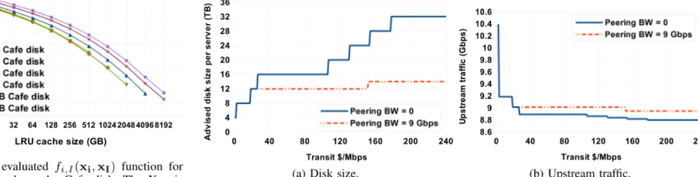
fi,I(xi,xI)for the interior LRU layers (i < I).fI(xI)for the Cafe-based disk (not shown here) is also a curve descending with disk size, though of different convexity [16]. In Figure 4, bold points represent simulated points forfi,I(xi,xI), based on which any other value is interpolated in the remaining small ranges. Since log-scale increments of xi values suffices for obtaining thefi,I(·)curve, this function can be estimated for the full range of inputs with limited simulations. We use2×

increments ofxi as shown in Figure 4. The total number of required simulations were less than100 which altogether took less than a day to run on the traces on a commodity PC. B. Results

We first examine how a server configured by the optimizer would operate in practice. A summary of this experiment is as follows; the detailed report is given in [16]. We consider the optimization of a 4 Gbps server’s cache layers for

Dmax=8 Gbps peak-time demand and B=4 Gbps peering bandwidth. We assumeC= $18/Mbps total transit cost based on a $0.50/Mbps projected monthly cost for the near future5

and a 3-year lifetime expectancy of a server deployment before replacement with newer hardware. We also assumeǫ = 0.1. The optimized output for this setting is 8 TB of disk cache as 4 drives, 2 TB of flash as 2 drives and a 64 GB RAM chip. The results of simulating this server on the traces confirm the validity of the optimization output in operation: r/w loads of disk and flash drives are within bandwidth limits, upstream traffic is as estimated, and the optimizer has arranged disk and flash drives such that they are utilized close to their limits.

Next, we analyze the tradeoff between network and storage cost. To isolate these costs from other factors, we suppose no peering bandwidth in the first experiment and no cost for higher layer caches. Disk r/w bandwidth is temporarily assumed

8 16 32 64 128 256 512 1024 2048 4096 8192 0 10 20 30 40 50 60 70 80 90 100

LRU cache size (GB)

P e a k -t im e f il l to e g re s s r a ti o ( % )

Fig. 4. The evaluatedfi,I(xi,xI) function for

all LRU layers above the Cafe disk. The X axis representsxiand each curve a differentxIvalues.

0 40 80 120 160 200 240 0 4 8 12 16 20 24 28 32 36 Transit $/Mbps A d v is e d d is k s iz e p e r s e rv e r (T B )

(a) Disk size.

0 40 80 120 160 200 240 8.6 8.8 9 9.2 9.4 9.6 9.8 10 10.2 10.4 10.6 Transit $/Mbps U p s tr e a m t ra ff ic ( G b p s ) (b) Upstream traffic.

Fig. 5. Optimal disk per server and the corresponding upstream traffic as transit cost (C) grows.

high enough so only disk space matters. Figure 5a plots the required disk space as transit cost C grows; see the curve labeled as 0 peering bandwidth. The figure corresponds to the serving of 40 Gbps user demand by a large rack of 8

servers, each with up to 32 TB of disk. Figure 5b shows the corresponding amounts of upstream traffic including the 8 Gbps excess demand. Figure 5 shows that even for such high transit costs as $50–100, adding more and more cheap disk space is not the best solution. Only for unrealistically expensive transits costs a disk space of 32 TB is advised. A noticeable pause is observed in Figures 5a and 5b on disk sizes 8, 16 and 32 TB, which is due to our discretization of thefi,I(xi,xI)function to these values and interpolating the in-between based on them. Nevertheless, this loss of visual smoothness makes negligible difference (<0.5%) in the overall optimized cost.

While this helps isolating disk space versus network cost, in a more realistic case there would exist some peering bandwidth to make up for the 8 Gbps excess demand as well as the servers’ cache-fill and redirected traffic. We therefore consider

8+1 = 9Gbps of peering bandwidth in the next experiment, shown by the dotted curves in Figure 5. It shows that increasing the disk size per server to beyond 12 TB is not necessary for a transit cost as high as $150. This is because the resultant upstream traffic is almost within the 9 Gbps peering bandwidth and exceeds it by only 20 Mbps. If the transit cost continues to grow beyond $150, the optimizer adds another 2 TB to the disk space to further cut that 20 Mbps of traffic. This shows how the right disk size to provision is a function of the existing peering bandwidth. If this bandwidth was below 8 Gbps in this experiment, we had to keep adding disks as transit cost grew; if it was beyond 10 Gbps, there would barely be any need for larger disk space than 2 to 4 TB. The joint optimization of cache and peering is analyzed at the end of this section.

We analyze when and to what size each cache layer is cost effective based on its r/w bandwidth and price. Table III shows sample results based on one server and 4 Gbps demand, although the results hold irrespectively [16]. Table III shows that if the r/w bandwidth of disk drives reduces by half, simply a higher number of smaller disks are prescribed. If the disk bandwidth doubles, though, the optimal configuration changes more radically to 6 (versus 4) disk drives of 2 TB, whose total throughput eliminates the need for higher layers. This significantly reduces the total cost by $1,700. More expensive disk prices do not change the optimization result

unless (trivially) if exceeding flash price—not shown in the table. That is, a multifold increase in disk price from0.1 to

0.5$/GB is still not worth reducing the disk space and incurring the more expensive cost of transit traffic. Reducing the disk price similarly does not affect the optimization output unless if done by several times, as shown in the table.

There will be no need for a memory cache if flash drives can read and write~30–50% faster than we considered. This would allow distributing the load of memory cache in part on more disk drives (6) and in part on the now-faster flash drives. Slower flash, on the other hand, would require a larger memory cache which is not as cost effective as just distributing the load of the flash layer over a higher disk count (8) and more RAM (192 GB), as shown in the table. Flash price per GB governs a tradeoff between how much flash or RAM to employ. Only a 40% increase in this price renders flash ineffective altogether, and a 40% decrease makes an all-flash cache atop disk with no RAM the preferred choice. The results also show that PCM SSDs could be a replacement for flash drives if the problem with their limited write bandwidth is solved—if they can write at least 1.3 Gbps in this experiment. With 1.5 Gbps write speed, they could replace the memory cache as well (not shown in the table). If in addition to higher write throughput (1.3 Gbps), PCM chips also reduce in price from $2/GB to $0.80/GB or less, there will be no need for a memory cache. The table also shows that less expensive RAM by only 20% or more would eliminate the need for any lower layer cache until disk, while more expensive RAM by 40% or more enforces larger flash drives to make the expensive RAM unnecessary.

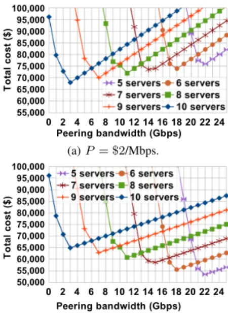
Finally, we analyze the peering bandwidth to provision to a server location based on the joint cost of server and peering provisioning—whereB is a target variable. The cost of peering provisioning isP $/Mbps and can be either that of installing routers and cables or renting peering ports at IXPs. In the first experiment, we assume P = $2/Mbps: about an order of magnitude less than transit cost (C= $36/Mbps). We also assume 40 Gbps peak demand and a $4000 server cost (w≃ $1/Mbps) including hardware and/or hosting premium (§V-A).

Figure 6a illustrates the results where each curve represents a fixed server count and each data point on the curve an optimized output: the peering bandwidth on the X axis and the total cost (servers, cache layers, peering and transit) on the Y axis. In each curve, the optimal peering bandwidth is at the minimum point: a bandwidth just enough to accommodate the

Configuration Disk Flash PCM RAM Cost ($) Upstream Default (Table II) 8 T /4 2 T /2 0/0 64 G /1 9,410 152 Mbps Disk r/w→200/150 Mbps 8 T /8 2 T /2 0/0 64 G /1 9,500 152 Mbps Disk r/w→800/600 Mbps 12 T /6 0/0 0/0 0/0 7,697 130 Mbps Disk $/GB: 0.10→_{0.02 16 T /4 4 T /2 0/0 16 G /1 8,633 115 Mbps} Flash r/w→4/1.5 Gbps 12 T /6 1 T /2 0/0 0/0 8,317 130 Mbps Flash r/w→2/0.7 Gbps 8 T /8 0/0 0/0 192/3 9,654 152 Mbps Flash $/GB: 0.50→_{0.3 12 T /3 4 T /2 0/0 0/0 8,803 130 Mbps} Flash $/GB: 0.50→_{0.7 8 T /8 0/0 0/0 192 G /3 9,654 152 Mbps} PCM write→_{1.3 Gbps 8 T /8 0/0 512 G /2 32/1 9,212 152 Mbps} PCM (1.3w) $/GB→_{0.80 12 T /6 0/0 1 T /2 0/0 8,516 130 Mbps} RAM $/GB: 10.00→8.00 8 T /8 0/0 0/0 192 G /3 9,270 152 Mbps RAM $/GB: 10.00→_{14.00 12 T /3 4 T /2 0/0 0/0 9,622 130 Mbps} Transit $/Mbps: 18→7 5 T /5 2 T /2 0/0 16 G /1 7,732 256 Mbps Transit $/Mbps: 18→28 12 T /3 4 T /2 0/0 0/0 10,925 130 Mbps TABLE III

CHANGES IN BANDWIDTH AND PRICE THAT MAKE A STORAGE TECHNOLOGY COST(IN)EFFECTIVE FOR USE AS A CACHE LAYER. THE BOLD-FACED ROW REPRESENTS THE BASE CONFIGURATION. THE THIRD ROW READS AS FOLLOWS:IF THE READ/WRITE BANDWIDTH PER DISK DRIVE WERE200/150 MBPS INSTEAD OF THE DEFAULTS OF400/300 MBPS,THE OPTIMAL CONFIGURATION WOULD BE8 TBOF DISK CACHE AS8DRIVES, 2 TBOF FLASH ABOVE IT AS2DRIVES,NOPCMCACHE, 64 GBOF MEMORY,

AND THIS WOULD YIELD A TOTAL COST OF$9,410AND AN UPSTREAM TRAFFIC OF152 MBPS. SERVER HARDWARE COST IS ASSUMED$4000 (w≃_{$1/MBPS),TRANSIT COST$18/MBPS AND NO PEERING.}

0 2 4 6 8 10 12 14 16 18 20 22 24 55,000 60,000 65,000 70,000 75,000 80,000 85,000 90,000 95,000 100,000 Peering bandwidth (Gbps) T o ta l c o s t ($ ) (a)P= $2/Mbps. 0 2 4 6 8 10 12 14 16 18 20 22 24 50,000 55,000 60,000 65,000 70,000 75,000 80,000 85,000 90,000 95,000 100,000 Peering bandwidth (Gbps) T o ta l c o s t ($ ) (b)P= $1/Mbps.

Fig. 6. Peering bandwidth provisioning.

servers’ upstream traffic and the excess demand. Any smaller peering bandwidth to the left of the minimum point results in rapidly growing transit cost, and any larger bandwidth is over-provisioning and a (linearly increasing) waste of budget with no caching efficiency gain. Moreover, comparing the optimum across the curves shows how smaller server counts result in higher peering bandwidths necessary. It also shows the important tradeoff between provisioning more servers or more peering bandwidth to an ISP. In the current scenario, 10 servers and 3 Gbps of peering is the optimal choice—assuming the ISP is willing to host that many servers.

This tradeoff is inherently shaped by the relative price of peering provisioning and server cost (P and w). For example, Figure 6b redraws Figure 6a if we manage to provide peering at half price (P = $1/Mbps). In this case, providing more peering bandwidth than physical servers is the cost effective approach. Further experimentation with lower and higher peering costs show that with a server cost ofw≃$1/Mbps and storage costs as in Table II, for P≥$1.6/Mbps it is always better to deploy the maximum number of servers (10) for the 40 Gbps demand; for P≤$1.4/Mbps it is best to deploy the least number of servers (1) and instead install more peering for the excess demand; P ≃$1.5/Mbps balances the cost of peering and server provisioning across different server counts—the CDN operators could go either way.

VII. CONCLUSIONS

We have studied the provisioning of a cluster of video CDN servers. We first analyzed the interaction of cache layers in a server, such as SSD and RAM above the disks, using actual server traces from a global video CDN. We found that the behavior of a cache layer can change significantly depending on its lower layers, but it changes only marginally by the addition of a higher layer which in turn will take a significant read load off. We designed an optimization framework to find the right server configuration and server count (and peering

bandwidth) to deploy at a given location. We have verified the validity of the prescribed configuration and we analyzed the optimal configuration along a variety of parameters involved including transit bandwidth cost, peering capacity, and storage r/w bandwidths and prices for disk, flash, PCM and RAM.

REFERENCES

[1] Akamai facts & figures. www.akamai.com/html/about/facts_figures.html. [2] peering.google.com/about/delivery_ecosystem.html, 2015.

[3] Akamai peering, 2015. www.akamai.com/peering.

[4] Google Global Cache program. peering.google.com/about/ggc.html, 2015. [5] A. Wolman et al. On the scale and performance of cooperative web

proxy caching. InProc. of ACM SOSP’99.

[6] J. Almeida, D. Eager, M. Ferris, and M. Vernon. Provisioning content distribution networks for streaming media. InIEEE INFOCOM’02. [7] D. Applegate et al. Optimal content placement for a large-scale VoD

system. InACM CoNEXT’10.

[8] E. Nygren et al. The Akamai network: A platform for high-performance internet applications. ACM SIGOPS Oper. Sys. Rev., 44(3):2–19, 2010. [9] P. Gill, M. Arlitt, Z. Li, and A. Mahanti. YouTube traffic characterization:

a view from the edge. InACM IMC’07.

[10] H. Kim et al. Evaluating phase change memory for enterprise storage systems: A study of caching and tiering approaches. InUSENIX FAST’14. [11] J. Ni et al. Large scale cooperative caching and application-level multicast in multimedia CDNs. IEEE Communications, 43(5):98–105, May 2005. [12] P. Jelenkovic and X. Kang. Characterizing the miss sequence of the LRU cache. ACM SIGMETRICS Perf. Eval. Review, 36(2):119–121, 2008. [13] K. Lim et al. Joint optimization of cache server deployment and request

routing with cooperative content replication. InIEEE ICC’14. [14] D. Karger et al. Web caching with consistent hashing. Computer

Networks, 31(11-16):1203–1213, 1999.

[15] T. Kelly and D. Reeves. Optimal Web cache sizing: scalable methods for exact solutions.Computer Communications, 24(2):163–173, 2001. [16] K. Mokhtarian. Content Management in Planet-Scale Video CDNs. PhD

thesis, University of Toronto, 2015.

[17] K. Mokhtarian and H.-A. Jacobsen. Caching in video CDNs: Building strong lines of defense. InEuroSys’14.

[18] N. Laoutaris et al. On the optimization of storage capacity allocation for content distribution. Computer Networks, 47(3):409–428, 2005. [19] G. Pallis and A. Vakali. Insight and perspectives for content delivery

networks. Communications of the ACM, 49(1):101–106, January 2006. [20] S. Agarwal et al. Volley: automated data placement for geo-distributed

cloud services. InUSENIX NSDI’10.

[21] S. Vanichpun and A. Makowski. The output of a cache under the independent reference model: Where did the locality of reference go?