Future Generation Computer Systems

(1)

journal homepage:www.elsevier.com/locate/fgcs

Characterizing spot price dynamics in public cloud environments

Bahman Javadi

a,∗

,

Ruppa K. Thulasiram

b

,

Rajkumar Buyya

c a_{School of Computing, Engineering and Mathematics, University of Western Sydney, Australia}

b_{Computational Financial Derivatives (CFD) Laboratory, Department of Computer Science, University of Manitoba, Winnipeg, Canada}

c_{Cloud Computing and Distributed Systems (CLOUDS) Laboratory, Department of Computing and Information Systems, The University of Melbourne, Australia}

a r t i c l e i n f o Article history:

Received 3 February 2012 Received in revised form 6 May 2012

Accepted 11 June 2012 Available online 14 July 2012

Keywords: Cloud computing Spot instances Spot price Statistical model Amazon’s EC2

a b s t r a c t

The surge in demand for utilizing public Cloud resources has introduced many trade-offs between price, performance and recently reliability. Amazon’s Spot Instances (SIs) create a competitive bidding option for public Cloud users at lower prices without providing reliability on services. It is generally believed that SIs reduce monetary cost to the Cloud users, however it appears from the literature that their characteristics have not been explored and reported. We believe that characterization of SIs is fundamental in the design of stochastic scheduling algorithms and fault tolerant mechanisms in public Cloud environments for the spot market. In this paper, we have done a comprehensive analysis of SIs based on one year price history in four data centers of Amazon’s EC2. For this purpose, we have analyzed all different types of SIs in terms of spot price and the inter-price time (time between price changes) and determined the time dynamics for spot price in hour-in-day and day-of-week. Moreover, we have proposed a statistical model that fits well these two data series. The results reveal that we are able to model spot price dynamics as well as the inter-price time of each SI by a mixture of Gaussians distribution with three or four components. The proposed model is validated through extensive simulations, which demonstrate that our model exhibits a good degree of accuracy under realistic working conditions.

1. Introduction

Due to the surge in demand for using utility computing systems like public Cloud resources, many trade-offs between price and performance have emerged. One particular type of Cloud service, which is known as Infrastructure-as-a-Service (IaaS) provides raw computing with different capacity and storage in the form of Virtual Machines (VMs) with various prices on a pay-as-you-go basis. For instance, Amazon provides on-demand and reserved VM instances, which are associated with a fixed set price [1]. However, Amazon can increase or decrease these prices based on their own local policy. There are 64 different types of instances with various capacities and prices under two operating systems (i.e. 32 for Linux and 32 for Windows) which are made available by Amazon in four data centers as illustrated inTable 1(sorted by their prices).1In this Table, the prices are given for the Linux operating system and the instances labeled with ‘m1’, ‘m2’, and ‘c1’ are standard, high-memory, and high-CPU instances, respectively.

In December 2009, Amazon released a new type of instances called Spot Instances (SIs) to sell the idle time of Amazon’s EC2

∗_{Corresponding author. Tel.: +61 2 9685 9181; fax: +61 2 9685 9245.}

E-mail address:[email protected](B. Javadi).

1 Amazon now has seven data centers around the world, but the four major data centers are considered in this research.

data centers [2]. The price of an SI, spot price, depends on the type of instance as well as VM demand within each data center. In fact, spot instances are an alternative to the other two classes of instances which offer a low price but less reliable and competitive bidding option for the public Cloud users. Therefore, another aspect,reliability, has been added to the existing trade-offs to make utility computing systems more challenging than ever.

In order to utilize SIs, the Cloud users provide abidwhich is the maximum price to be paid for an hour of usage. Whenever the current price of an SI is equal or less than the user bid, the instance is made available to the user. If the price of an SI becomes higher than the user’s bid,out-of-bidevent (failure), the VM(s) will be terminated by Amazon automatically and the user does not pay for any partial hour. However, if the user terminates the running VM(s), she has to pay for the full hour. Amazon charges users per hour by the market price of the SI at the time of VM creation.

There are a number of works on how to utilize SIs to decrease the monetary cost of utility computing for Cloud users [3–5]. However, a thorough statistical analysis and modeling of SIs have not appeared in the literature, the focus of our research in this study. In this paper, we provide a comprehensive analysis of all SIs in terms of spot price and the inter-price time (time between price changes) in four Amazon data centers (i.e. us-west, us-east, eu-west, and ap-southeast). Moreover, we propose a statistical model to capture the volatile spot prices in Amazon’s data centers. The main contributions of this paper are as follows:

(2)

m1.xlarge 76 68 76 76 8 15 1690

c1.xlarge 76 68 76 76 20 7 1690

m2.2xlarge 114 100 14 114 13 34.2 850

m2.4xlarge 228 200 228 228 26 68.4 1690

•

We provide statistical analysis for all SIs in Amazon’s EC2 data centers. We also determine the time correlation in spot price in terms of hour-in-day and day-of-week.

•

We model spot price and the inter-price time of each SI with a mixture of Gaussians distribution. A model calibration algorithm is also proposed to deal with an observed price trend in the real price history.

•

We validate and verify the accuracy of our proposed model through simulation under realistic working conditions. We believe that results of this research will be significantly helpful in the design of stochastic scheduling algorithms and fault tolerant mechanisms (e.g. checkpointing and replication algorithms) for the spot market in public Cloud environments. In addition, although Amazon is the only provider of SIs at the moment, some research has been conducted to analyze the free computing resource markets [6,7]. So, this model can be used by other resource providers that look to offer such a service in the near future.

The paper is structured as follows. In Section2, we describe the processes that we model in this paper. We discuss related work in Section3. We examine the pattern of spot price in Section4. In Section5, we present the global statistics for all SIs. We then illustrate distribution fitting for spot price and the inter-price time in Section 6. In Section7, we propose an algorithm for model calibration. We discuss the validation of the proposed models through simulation in Section8. In Section9, we summarize our contributions and describe future directions.

2. Modeling approach

In this section, we describe two variables that we are going to analyze and model. In Amazon’s data centers, SIs have two variables (i.e. spot price and inter-price time) specified by the Cloud provider and one variable (user’s bid) determined by users. In this study, we focus on the analysis and modeling of spot price and the inter-price time as two highly volatile system variables. These variables are illustrated inFig. 1wherePiis the price of an SI at timeti. So, the inter-price time is defined asTi

=

ti+1

−

ti. Therefore, the time series of spot price (Pi) and the inter-price time (Ti) are analyzed and modeled in the following sections.

The traces that we use in this study are one year price history of all Amazon SIs from the first of February 2010–mid-February 2011. We use the first 10 months (Feb-2010–Nov-2010) in the modeling process. These 10-month traces along with the last 2 months are used for the model validation purpose. The spot price history is freely provided by Amazon per SI for each data center and also available through other third parties such as [8]. We do not use data prior to February 2010 due to an algorithm issue reported in [9] for prices. Moreover, we only use the SIs with Linux operating systems from all data centers. Due to the similarity of the results, we present our findings for only two data centers (i.e. eu-west and us-east). Interested readers can refer to the extended version of this paper [10] for more discussion about other data centers.

Fig. 1. Spot price and the inter-price time of Spot Instances.

3. Related work

Although the current literature shows that SIs are a good alter-native for on-demand or reserve instances in terms of monetary cost, the characteristics of SIs are still not clear to users and re-searchers in the community. Wee [11] considered SIs as computing resources with real-time pricing. Focusing on the real price history of SIs, this paper concluded that still users need more monetary incentive to shift their workload into SIs. Another work that inves-tigated the behavior of spot prices is presented in [12], where the authors used reverse engineering to construct a price model based on the Auto-Regressive (AR) model for SIs.

Our work is different in several aspects. We provide statistical analysis of all SIs and study their behavior in terms of hour-in-day and hour-in-day-of-week. Moreover, we propose to devise a statistical model for spot price as well as inter-price time. In addition, the simulation results reveal that we are able to model behavior of SIs by a mixture of Gaussians with three or four components.

In the following, we briefly review the other related work mainly investigating the usage of SIs to decrease the monetary cost of utility computing. Yi et al. [3,4] introduced some checkpointing and migration mechanisms for reducing the cost of SIs. They used the real price history of EC2 spot instances and showed how the adaptive checkpointing and migration schemes could decrease the monetary cost and improve the job completion times. Chaisiri et al. [13] proposed two provisioning algorithms based on stochastic programming, robust optimization, and sample-average approximation to optimized the provisioning cost for long-term and short-term planning. Moreover, in [14], a resource allocation policy to run deadline constrained jobs on SIs in a cost-effective manner is proposed.

In [15], a decision model for the optimization of performance, cost and reliability under SLA constraints while using SIs is proposed. They used the real price history and workload models to demonstrate how their proposed model can be used to bid optimally on SIs to reach different objective with desired levels of confidences. Mazzucco and Dumas [16] considered a case where a web service is deployed on SIs and proposed a bidding schema and

(3)

(a) Hour-in-day. (b) Day-of-week.

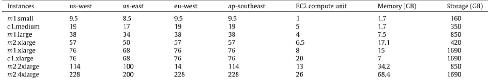
Fig. 2. Patterns of spot price in eu-west data center.

resource allocation policies to optimize the web service provider’s revenues.

Chohan et al. [17] proposed a method to utilize the SIs to speed up the MapReduce tasks. They provided a Markov chain to predict the expected lifetime of an SI. They concluded that having a fault tolerant mechanism is essential to run MapReduce jobs on SIs. Also, in [5], the authors proposed a hybrid Cloud architecture to lease the SIs to manage peak loads of a local cluster. They proposed some provisioning policies and investigated the utilization of SIs compared to on-demand instances in terms of monetary cost saving and number of deadline violations.

Zhang et al. [18,19] investigated the dynamic market control problem in a single cloud provider motivated by the SIs offered by Amazon’s EC2. They used static and dynamic optimizations for resource allocation to maximized the provider’s revenue as well as user satisfactions. Rahman et al. [20] proposed resource allocation for Cloud users based on financial option theory to reduce the risk of dynamic price in spot markets. They showed that fluctuation in Amazon’s SIs are much lower than expected values in a free market. This possibly is because of less users for SIs in comparison to other types of reliable resources such as on-demand instances.

Statistical modeling has been widely used in the characteri-zation of computer systems’ workloads and failures [21–23]. Al-though we apply the same techniques, the characteristics of SIs are far from the behavior of the workloads and failures, so require a comprehensive analysis.

4. Patterns of spot price

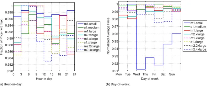
In this section, we examine hour-in-day and day-of-week time dynamics for the price of different SIs in eu-west and us-east data centers. We use the same approach as [24] to show how the price of one SI changes each hour in the day or each day of the week. As we have the price history in GMT time zone, we adjusted the local time for the time zone. This adjustment could reveal the dependency of spot price on the local time of a data center.

InFigs. 2(a) and3(a), we create eight 3-h time slots per day, and determine the average price of each SI in each time slot over all days. Then, we normalized this average by the maximum average price over all days. Note that the frequency of 3-h sampling could be increased to 1-h sampling with 24 time slots in a day. However, it would only increase the sample size without shedding much light on the price dynamics, since spot prices in Amazon’s data centers change at most every 2–3 h (see Section5). In these figures, we can observe that they-axis is in the range of [0.98 1.0] where

there is an increasing trend over the first half of each day ([0 12]) and a decreasing trend in spot price during the second half of each day for all SIs in each data center.

InFigs. 2(b) and3(b), we applied the same procedure to obtain the average price over seven 24-h time slots within a week. The

y-axis in these figures has a wider range of [0.91 1.0] for eu-west and [0.95 1.0] for us-east data centers.2As it is observable from this plot, we can not find any specific pattern for spot price in eu-west, except the decreasing prices on weekends. However, for other Amazon’s data centers such as us-east, we see more clear patterns in day of the week where on Tuesday we have the maximum price for almost all SIs in those data centers. Moreover, the lowest price are on Saturday, but on Sunday we again observe increasing price for all SIs.

5. Global statistics and analysis

In the following, we analyze the price history of different SIs in eu-west and us-east data centers. It has been shown that spot prices tend to be random rather than market-driven [12]. So, analysis of global statistics can reveal some basic facts about SIs.3

We inspect the basic statistics of the traces in terms of spot price inTables 2and 3; and in terms of the inter-price time in

Tables 4and5. The statistics in the tables are mean, trimmed mean (the mean value after discarding 10% of extreme values), median, standard deviation (Std), coefficient of variance (CV), interquartile range (IQR), maximum, minimum, skewness (the third moment), kurtosis (the fourth moment) and number of samples.

These tables show three types of descriptive statistics. Statistics of the first type (mean, median, trimmed mean) reveal the central tendency of the distributions. The trimmed mean is a useful estimator of the central tendency as it is less sensitive to outliers. Statistics of the second type (CV, IQR, minimum, maximum) reflect the spread of the distributions. Statistics of the third type (kurtosis, skewness) represent the shape of the distributions.

First of all, we find that on average the price of SIs can be as low as 44% and 38% of on-demand instances for eu-west and us-east data centers, respectively. This expresses that there are some opportunities in reducing monetary cost of utility computing at

2 For other data centers, this range is ([0.95 1.0]).

3 We conduct all of our statistical analysis using Matlab R2010b on a 32-bit Core2Duo 3.00 GHz desktop with 3 GB of RAM. We use when possible standard tools provided by the Statistical Toolbox. Otherwise, we implement or modify statistical functions ourselves.

(4)

(a) Hour-in-day. (b) Day-of-week.

Fig. 3. Patterns of spot price in us-east data center.

Table 2

Statistics for spot price in the eu-west data center (values given in cents).

Instances Mean TrMean Median Std CV IQR Max Min Skewness Kurtosis No

m1.small 4.00 4.00 4.00 0.19 0.05 0.20 9.50 3.80 9.44 242.97 3702 c1.medium 8.00 8.00 8.00 0.27 0.03 0.40 10.10 7.60 0.28 3.91 3812 m1.large 16.04 16.02 16.10 0.85 0.05 1.00 50.00 15.20 21.55 792.41 3875 m2.xlarge 24.04 24.03 24.10 1.03 0.04 1.40 57.10 22.80 12.91 387.69 3763 m1.xlarge 32.05 32.01 32.10 1.60 0.05 2.00 76.00 30.40 15.34 415.47 3917 c1.xlarge 32.04 32.03 32.10 1.07 0.03 2.00 45.00 30.40 0.54 8.27 3658 m2.2xlarge 56.04 56.04 56.20 1.83 0.03 3.42 76.00 53.20 0.25 4.99 4001 m2.4xlarge 112.08 112.08 112.50 3.62 0.03 6.80 150.00 106.40 0.21 4.55 3912 Table 3

Statistics for spot prices in the us-east data center (values given in cents).

Statistics for the inter-price time in the eu-west data center (values given in hours).

Statistics for the inter-price time in the us-east data center (values given in hours).

m1.small 2.22 1.66 1.36 3.53 1.59 0.32 76.59 0.78 9.21 130.29 3278 c1.medium 2.00 1.65 1.37 2.09 1.05 0.31 49.91 1.00 6.91 98.48 3642 m1.large 3.58 2.20 1.44 18.60 5.20 1.54 657.29 1.00 26.29 824.35 2033 m2.xlarge 1.91 1.58 1.34 2.02 1.06 0.31 36.26 1.00 6.11 61.19 3523 m1.xlarge 1.96 1.62 1.34 3.05 1.55 0.32 145.98 0.58 30.51 1370.41 3703 c1.xlarge 2.02 1.66 1.35 3.38 1.67 0.33 171.62 1.00 35.74 1758.12 3599 m2.2xlarge 1.92 1.62 1.34 1.94 1.01 0.31 50.40 1.01 8.42 143.99 3789 m2.4xlarge 1.92 1.62 1.35 1.76 0.92 0.32 23.02 1.00 4.50 30.98 3789

(5)

(a)m1.small. (b)c1.medium. (c)m1.large. (d)m2.xlarge.

(e)m1.xlarge. (f)c1.xlarge. (g)m2.2xlarge. (h)m2.4xlarge.

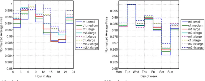
Fig. 4. Probability density functions of spot price for all SIs in the eu-west data center.

the cost of unreliability. Moreover, the maximum price of some SIs (likem1.large) is bigger than the price of corresponding on-demand instance (especially in the east data center). Since us-east is the cheapest data center, more user demand increases the fluctuation in spot prices. (The higher value of CV in spot prices in us-east confirms this variability.) Thus, even if the users’ bid is as high as the on-demand prices, we may still have a probability of out-of-bid events.

The results in these tables reveal that the ratios between the mean and the median for spot price and the inter-price time of SIs are close to 1 for each trace. This indicates that a Gaussian distribution might be a good option for the model. However, the skewness and kurtosis values show that the underlying distributions are right skewed and short tailed. Therefore, a Gaussian distribution may not be a representative model to use and a better distribution is in order.

Additionally, we can observe that the inter-price time is more variable than spot price due to higher values of coefficient of variance. Also, analysis of the trimmed mean confirmed that inter-price time has greater variability. Therefore, we may need distributions with higher degrees of freedom, to model the inter-price time for these traces. It is worth noting that the minimum inter-price time is almost one hour in all data centers except eu-west which is about a few minutes and can be seen inTable 4. Moreover, in eu-west and us-east data centers, the set prices of SIs are stable on average for 2–3 h. This observation is valid for other data centers as well [10]. This is the justification of 3-h time slots to examine patterns of spot price inFigs. 2(a) and3(a).

6. Distribution fitting

After global statistical analysis, we first inspect the Probability Density Function (PDF) of spot price and the inter-price time. Then, we conduct parameter fitting for the Mixture of Gaussians (MoG) distribution by the expectation maximization (EM) algorithm to model both time series. We considered other distributions, such as Weibull, Normal, Log-normal and Gamma distributions as well. However, the mixture of Gaussians distribution shows better fit with respect to the others [10]. In this section, we show the process of fitting for the eu-west data center to avoid presenting similar figures and plots. We present the final results for both selected data centers.

6.1. Probability densities

The PDFs of spot price of each SI in the eu-west data center are depicted inFig. 4. We can easily observe bi-modalityin the probability density functions. Moreover, the price distribution of all SIs, exceptm1.small, are almost symmetric. The exception for

m1.small is possibly because of diverse usage patterns of this instance as the cheapest resource in each data center.

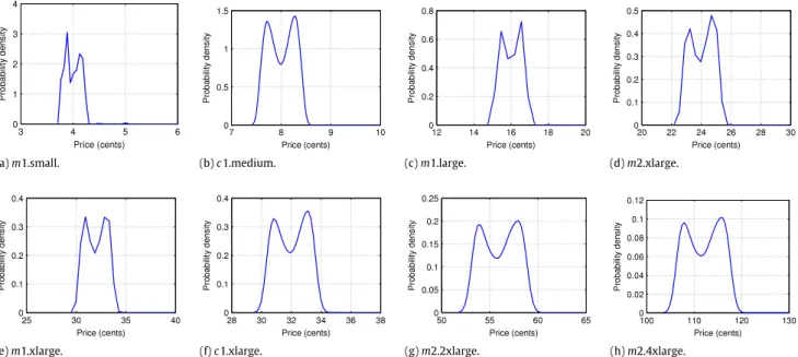
The PDFs of the inter-price time for each SI in eu-west are represented inFig. 5. Obviously, there is a single dominant mode (peak) in the density functions when compared to (nearly) equal peaks in the PDFs of spot price. Most SIs have the peak around two hours, which confirms the results of the previous section (see Mean column inTable 4). The reason for the very sharp peak in these density functions is investigated in Section7. Observing the plotted density functions of both time series, our decision to propose a mixture of Gaussians distribution as a good candidate for approximating such density shapes is further strengthened. This is also confirmed by Li et al. [25] where they used a mixture of Gaussians distribution to model amulti-modaldensity function.

6.2. Parameter estimation and goodness of fit tests

In this section, we conduct parameter fitting for the mixture of Gaussians distribution withkcomponents, which is defined as follows: cdf

(

x

;

k

,

⃗

p

,

µ,

⃗

σ

⃗

2

)

=

k



i=1 pi 2



1

+

erf



x

−

µ

_i

σ

i

√

2



(1)

where

µ

⃗

,

σ

⃗

2_{, and}_p

⃗

_{are the vectors of mean, variance and}

proba-bility of components withkitems. Also,erf

()

is the error function, which is defined as follows:

erf

(

x

)

=

√

2

π



x

0

e−t2dt

.

(2)

To maximize the data likelihood in terms of parameters

µ

⃗

and

σ

⃗

2 _where _k _{is given a priori, we adopt the expectation}

maximization (EM) algorithm, which is a general maximum likelihood estimation [21]. Parameter fitting was done using Model Based Clustering (MBC), which was introduced by Fraley and

(6)

Fig. 5. Probability density functions of the inter-price time for all SIs in the eu-west data center.

Raftery [26]. MBC is a methodological framework that can be used for data clustering as well as (multi)variate density estimation. One assumption is that data has several components each of which is generated by a probability distribution. Model Based Clustering uses Bayesian model selection to choose the best model in terms of number of components [25]. In contrast, we use the goodness of fit (GOF) tests to determine the best model as we have an estimation for the number of components in the model. We choose the number of components between 2 and 4 (2

≤

k

≤

4) based on the observation of the density functions. We measured the goodness of fit of the resulting models using a visual method (i.e. standard probability–probability (PP) plots) and Kolmogorov–Smirnov (KS) and Anderson–Darling (AD) tests [21] as quantitative metrics.

After parameter estimation, we must examine the quality of each fit through GOF tests. First of all, we present the graphical results of distribution fitting for spot price and the inter-price time of all SIs inFigs. 6and7for the eu-west data center, respectively. In these plots, the closer the plots are to the liney

=

x, the better the fit. In each plot thex-axis is the empirical quantiles while the

y-axis is the fitted quantiles. Based on these figures, a mixture of Gaussians distribution with three or four components can fit the spot price and the inter-price time of SIs in the eu-west data center. The only instance which is hard to fit, especially in terms of spot price, is them1.small instance.

To be more quantitative, we also report thep-values of two GOF tests (i.e. KS and AD tests). We randomly select a subsample of 50 from each trace, compute thep-values iteratively 1000 times and finally obtain the averagep-value. This method is similar to the one used by the authors in [27]. Moreover, in all cases the coefficient of variance is less than one (i.e.,CV

<

1), so the average value is a representative estimate.

The results of GOF tests are listed inTables 6and7for spot price in eu-west and us-east data centers. For the inter-price time, the

p-values are presented inTables 8and9in eu-west and us-east, respectively. Moreover, in each row the best fits are highlighted. In some cases, we have two winners as there is one best fit per GOF test. These quantitative results strongly confirm the graphical results of the PP-plots. Thep-values in the first row ofTables 6and

7express that the spot price of them1.small instance is hard to fit, even with four components.

The set of parameters for MoG distributions is listed inTables 10

and11for spot price and the inter-price time fork

=

3 in eu-west and us-east data centers, respectively. It is worth noting that in

Table 6

p-values resulting from KS and AD tests for spot price in eu-west.

Instances MoG (k=2) MoG (k=3) MoG (k=4)

m1.small 0.016 0.791 0.017 0.789 0.053 0.803 c1.medium 0.211 0.779 0.217 0.791 0.224 0.790 m1.large 0.113 0.678 0.319 0.752 0.354 0.754 m2.xlarge 0.139 0.616 0.356 0.721 0.415 0.734 m1.xlarge 0.134 0.570 0.369 0.708 0.431 0.706 c1.xlarge 0.394 0.681 0.444 0.705 0.421 0.707 m2.2xlarge 0.420 0.648 0.469 0.682 0.450 0.672 m2.4xlarge 0.429 0.617 0.463 0.637 0.476 0.653 Table 7

p-values resulting from KS and AD tests for spot price in us-east.

Instances MoG (k=2) MoG (k=3) MoG (k=4)

m1.small 0.000 0.732 0.000 0.736 0.000 0.727 c1.medium 0.056 0.774 0.150 0.796 0.147 0.797 m1.large 0.158 0.726 0.157 0.723 0.329 0.763 m2.xlarge 0.132 0.697 0.138 0.690 0.126 0.693 m1.xlarge 0.142 0.634 0.138 0.633 0.142 0.627 c1.xlarge 0.180 0.669 0.187 0.673 0.187 0.673 m2.2xlarge 0.169 0.553 0.433 0.693 0.453 0.699 m2.4xlarge 0.169 0.464 0.181 0.470 0.181 0.467

the list of parameters, we just report two items of parameter

⃗

p, as the last item in this vector can be computed using the others (i.e.pk

=

1

−



k−1

i=1pi).

As the number of parameters in the MoG distribution is 3k

+

1 (see Eq.(1)), we have a trade-off between accuracy and complexity of the model. With fewer components, the analysis becomes simpler that gives reasonably good fit to spot price and inter-price time with a compromise of accuracy to some extent. This would significantly help in understanding the data series on the first step. With this understanding a model to better fit the data series with many components can be designed. Hence, for the sake of simplicity and homogeneity, in the rest of this paper we choose the model with three components (k

=

3) for both spot price and the inter-price time for further analysis. The set of parameters for MoG

(7)

(a)m1.small. (b)c1.medium.

(c)m1.large. (d)m2.xlarge.

(e)m1.xlarge. (f)c1.xlarge.

(g)m2.2xlarge. (h)m2.4xlarge.

Fig. 6. PP-plots of spot price in eu-west for the mixture of Gaussians (k=2,k=3,k=4).X-axis: empirical quantiles, andY-axis: fitted quantiles.

Table 8

p-values resulting from KS and AD tests for inter-price time in eu-west. Instances MoG (k=2) MoG (k=3) MoG (k=4)

distributions for spot price and the inter-price time for 2

≤

k

≤

4 in all data centers is reported in [10].

7. Model calibration

In this section, we look into the time evolution of spot price and the inter-price time, which potentially can lead us to obtain a more accurate model. For this purpose, we examine the scatter plot of spot price and the inter-price time during February 2010 to November 2010. We just present the plots for them2.4xlarge instance, as the results are consistent for other instance types within the data centers.

Fig. 8(a) depicts the scatter plot of spot price form2.4xlarge in the eu-west data center for the duration of the price history. As can be seen in this figure, there is no clear correlation in spot price

Table 9

p-values resulting from KS and AD tests for inter-price time in us-east. Instances MoG (k=2) MoG (k=3) MoG (k=4)

where they are evenly distributed in a specific range (this range depends on the type of instances). However, congestion of spot price is increased after mid-July and this is the case for all SIs in the eu-west data center. To confirm this observation, we examine the scatter plot of the inter-price time for this SI inFig. 8(b). We observe that inter-price time become suddenly shorter after mid-July. That means, the frequency of changing price is increased while the spot price remains bounded within a small price range. The inspection of other SIs within the data center reveals the same result. This is also the reason for the very sharp peak in density functions of the inter-price time inFig. 5.

This trend is possibly due to some fine tunings made by Amazon in their pricing algorithm. It is worth noting that the same issue has been observed in other Amazon’s EC2 data centers oin different dates. As illustrated inFig. 9, this phenomenon is observable in

(8)

(c)m1.large. (d)m2.xlarge.

(e)m1.xlarge. (f)c1.xlarge.

(g)m2.2xlarge. (h)m2.4xlarge.

Fig. 7. PP-plots of the inter-price time in eu-west for the mixture of Gaussians (k=2,k=3,k=4).X-axis: empirical quantiles, andY-axis: fitted quantiles.

Table 10

Parameters of the mixture of Gaussians distributions for spot price and inter-price time in eu-west.

Instances Price model (k=3) Inter-price model (k=3)

⃗ p µ⃗ σ⃗2 _⃗_p _µ_⃗ _σ⃗2 m1.small 0.003 0.003 5.216 5.216 3.997 1.670 1.670 0.020 0.178 0.028 3.474 11.536 1.292 2.308 120.051 0.022 c1.medium 0.443 0.276 8.018 8.292 7.703 0.045 0.006 0.006 0.807 0.090 1.279 6.452 2.876 0.022 12.435 0.528 m1.large 0.492 0.505 15.556 16.470 24.401 0.059 0.048 114.879 0.068 0.126 6.793 3.040 1.276 13.803 0.940 0.022 m2.xlarge 0.445 0.001 23.264 53.500 24.643 0.109 12.960 0.135 0.824 0.066 1.284 2.506 5.166 0.022 0.035 8.192 m1.xlarge 0.457 0.002 31.010 53.803 32.848 0.184 326.523 0.249 0.793 0.177 1.283 3.310 8.356 0.022 1.864 29.730 c1.xlarge 0.261 0.243 33.188 30.756 32.057 0.072 0.058 0.722 0.811 0.187 1.286 4.048 84.430 0.022 5.341 15636.817 m2.2xlarge 0.492 0.252 56.119 53.784 58.100 1.813 0.157 0.216 0.405 0.399 1.155 1.398 4.044 0.007 0.008 6.795 m2.4xlarge 0.263 0.249 116.126 107.609 112.183 0.898 0.660 7.061 0.063 0.137 6.705 3.001 1.279 13.524 0.863 0.022 Table 11

Parameters of the mixture of Gaussians distributions for spot price and inter-price time in us-east.

Instances Price model (k=3) Inter-price model (k=3)

⃗ p µ⃗ σ⃗2 _⃗_p _µ_⃗ _σ⃗2 m1.small 0.024 0.952 6.009 3.012 6.009 3.402 0.009 3.402 0.164 0.043 3.581 13.935 1.301 2.638 120.212 0.025 c1.medium 0.439 0.537 5.808 6.167 8.726 0.007 0.011 2.935 0.780 0.145 1.301 2.954 7.379 0.023 0.814 20.600 m1.large 0.596 0.094 11.979 22.345 12.066 0.147 114.857 0.148 0.023 0.389 54.787 3.976 1.277 11982.593 4.795 0.022 m2.xlarge 0.461 0.504 17.020 17.020 38.737 0.299 0.299 209.027 0.147 0.814 3.508 1.282 9.249 1.809 0.023 27.356 m1.xlarge 0.008 0.439 41.511 24.045 24.023 425.466 0.591 0.593 0.778 0.015 1.278 13.908 3.655 0.022 353.873 3.005 c1.xlarge 0.071 0.328 51.722 24.064 24.028 340.120 0.594 0.593 0.759 0.016 1.280 14.298 3.651 0.021 459.583 3.196 m2.2xlarge 0.444 0.549 40.715 43.104 61.120 0.308 0.462 334.756 0.041 0.778 8.230 1.278 3.230 29.753 0.021 1.354 m2.4xlarge 0.594 0.007 83.823 166.323 84.275 7.063 2453.527 6.942 0.218 0.398 4.194 1.167 1.407 7.461 0.008 0.007

us-east at the end of July 2010 form2.4xlarge instances. Also, for us-west and ap-southeast data centers this change happened in January 2011 (figures are plotted in [10]).

Focusing on the scatter plot of the inter-price time (MoG model fork

=

3) presented inFig. 8(b), we can see that after mid-July

only one component (i.e. component 3) remains and the other components collapsed to a small band. As this observation is consistent over all SIs, we propose a model calibration algorithm (Algorithm 1) to find the date of collapse (which is called the calibration date) as well as the remaining component(s).

(9)

(a) Scatter plot of spot price form2.4xlarge. (b) Scatter plot along with the components’ distribution of the inter-price time form2.4xlarge.

Fig. 8. Scatter plot of spot price and inter-price time form2.4xlarge in eu-west.

(a) Scatter plot of spot price form2.4xlarge. (b) Scatter plot along with the components’ distribution of the inter-price time form2.4xlarge.

Fig. 9. Scatter plot of spot price and inter-price time form2.4xlarge in us-east.

The algorithm needs the trace of the inter-price time of an SI (Traceinst) and the number of components (k). The result of the mixture of Gaussians model with k components is

−−→

index. Also,

−

→

dateis a vector, each element of which corresponds to each item of

−−→

index. At first, the algorithm computes the probability of each component in each month in the whole trace and after that finds a list (

−

Q

→

_m) where the probability of one or more components is less thanq0(lines 4–8).q0is a threshold value and we define it as low

as 0.01 (i.e.q0

=

0

.

01). The components that are not in this list

are remaining components (

−−−→

RCmpsin line 10). The first month in the list of

−

Q

→

mis the calibration month, calledm(line 11). Finally, the last occurrence of the component(s) in monthmwould be the calibration date (CalDate), which is obtained in lines 13–19.

The results of applying this algorithm for all SIs in eu-west and us-east data centers are presented inTable 12where all calibration dates are in July. The remaining components can be inspected in the fifth column (

⃗

pof the inter-price time model) of Tables 10

and11, where the component(s) with higher probability remain(s)

beyond the calibration date. For instance, the third component of the inter-price time model for m2.4xlarge in eu-west with probability of 0.8 (1

−

0

.

063

−

0

.

137) remains after 15 July where the mean and variance are 1.279 and 0.022 h, respectively. The graphical demonstration ofFig. 8(b) can confirm the correctness of this algorithm, where component 3 implies a cluster around the mean value of 1.279 h.

The last step of the model calibration is probability adjustment where the probability of remaining component(s) must be scaled up to one. This adjustment can be done by the following formula:

pj

=

pj



∀i pi i

,

j

∈

−−−→

RCmps

.

(3)

In other words, in the calibrated model for each SI, we just change the probability of the remaining component(s) after the calibration date. In the following section, we investigate the accuracy of the calibrated model with respect to the real price history as well as the non-calibrated model.

(10)

4 index←(c1,c2, . . . ,cn) ci∈ {1, . . . ,k};

5

−−→

date←(d1,d2, . . . ,dn) di∈ {Ts. . .Te};

6 qa,b←probability of componentain monthb;

7 − → Q ←qa,b|a∈ {1, . . . ,k},b∈ {Ts. . .Te}  ; 8 −→ Qm← {qf,e|qf,e<q0,qf,e∈ − → Q}; 9 −−→ Cmps← {g|qg,h∈ −→ Qm}; 10 −−−→ RCmps← {1, . . . ,k} −−−→Cmps; 11 m←min{h|qg,h∈ −→ Qm};

12 //Traceinst(m) is the trace for month m;

13 Tms←Traceinst(m).start.time;

14 Tme ←Traceinst(m).end.time;

15 z←Sizeof(Traceinst(m));

16 −−−→ Sindex←(c′ 1,c ′ 2, . . . ,c ′ z) c ′ i ∈ {1, . . . ,k}; 17 −−→ Sdate←(d′ 1,d ′ 2, . . . ,d ′ z) d ′ i∈ {Tms. . .Tme}; 18 t←max{rl| −−−→ Sindex(rl)==g,l∈ {1, . . . ,z}}; 19 CalDate← −−→ Sdate(t); Table 12

The results of model calibration in eu-west and us-east (k=3). Instances Calibration dates Remaining components

eu-west us-east eu-west us-east

m1.small 24-July 25-July 3 1, 3

c1.medium 15-July 25-July 1 1

m1.large 15-July 26-July 3 2, 3

m2.xlarge 13-July 27-July 1 2

m1.xlarge 23-July 24-July 1 1

c1.xlarge 23-July 26-July 1 1, 3

m2.2xlarge 23-July 26-July 1, 2 2

m2.4xlarge 15-July 26-July 3 2, 3

8. Model validation

In order to validate the proposed model, we implemented a discrete event simulator using CloudSim [28]. The simulator has a general architecture of IaaS Cloud with the capability of provisioning of on-demand and Spot Instances for input workload. The simulator uses the model or the price history traces to run the input workload. We consider the case where the user requests one VM from one type of SI and runs whole jobs on that VM. The total monetary cost of running the workload on an SI is the parameter to be considered. In this section, we only present the results for eu-west. The validation results are the same for us-east and other data centers.

8.1. Simulation setup

The workload that we use in our experiments is the workload traces from LCG Grid which is taken from the Grid Workloads Archive [29]. We use the first 1000 jobs of this trace as the input workload for the experiments which is long enough to reflect the behavior of spot price for different SIs. We assume that one EC2 compute unit is the equivalent of a CPU core with capacity of 1000 MIPS.4_{We also assume that all jobs can be executed on a single}

VM, so we do not have any parallel jobs. As such, the selected

4 Amazon mentioned that one EC2 compute unit has equivalent CPU capacity to a 1.0–1.2 GHZ 2007 Opteron or 2007 Xeon processor [2].

bidevent in the execution of the given workload. We use the model with three components (k

=

3) for both spot price and the inter-price time to show the trade off-between accuracy and complexity. In our experiments, the results of the simulations are accurate with a confidence level of 95%.

8.2. Results and discussion

In the following, we present the results of two different sets of experiments. First, we discuss the results of model validation where we have the price history that was included in the modeling process (i.e. Feb-2010–Nov-2010). Second, we report the results from model validation using a new price history which was not included in the modeling process. The new price history is from December 2010 to mid-February 2011.

Fig. 10shows the model validation results where the probability density functions of the total monetary cost to run the given workload have been plotted for all types of SIs. In each plot, Trace, Model-Cal, and Model-nCal refer to the result of using the real price history, the model after calibration and the model before calibration, respectively. Based on these figures, the proposed models match the real trace simulations with a high degree of accuracy, especially for the calibrated models. As we can see in these plots, in all cases the calibrated models are the better match with the trace simulations. As we expect, there are discrepancies in the model and trace simulation results form1.small instance. However, the mean total cost for running the given workload for all SIs is very accurate where the maximum relative error is less than 3% for both calibrated and non-calibrated model, respectively.

Additionally, we report the model validation results where we use the new price history from December 2010 to mid-February 2011 to see the quality of the models for the future traces. The result of the simulations for the new price history are plotted inFig. 11. The results reveal that our models with three components still conform to the trace simulation results, except for them1.small instance. As mentioned earlier, the spot price for them1.small instance is hard to fit and this is the reason for this inaccuracy. This means that form1.small, we should use a model with more components (e.g. k

=

4) to get better accuracy. The calibrated models again match better with the trace simulations in comparison to the non-calibrated models for all SIs. Besides, the maximum relative error of the mean total cost for all SIs is less than 4% for both calibrated and non-calibrated models. Therefore, the proposed models are accurate enough for the new price history as well.

9. Conclusions

We considered the problem of discovering models for Spot In-stances in Amazon’s EC2 data centers for spot price and inter-price time. The main motivation behind this is to explore characteriza-tion of SIs that is essential in the design of stochastic scheduling algorithms and fault tolerant mechanisms (e.g. checkpointing and replication algorithms) in Cloud environments for the spot market. We studied the price patterns of Amazon’s data centers for a one year period and provided a global statistical analysis to get a bet-ter understanding of these patbet-terns. Based on this understanding and observed bi-modality in probability densities, we proposed a model with a mixture of Gaussians distribution with three or four

(11)

Fig. 10. Model validation for all SIs in eu-west for the modeling traces (Feb-2010–Nov-2010).

Fig. 11. Model validation for all SIs in eu-west for the new traces (Dec-2010–mid-Feb-2011).

components for eight different types of SIs. The proposed model is validated through simulations, which reveals that our model pre-dicts the total price of running jobs on spot instances with a good degree of accuracy. We believe that the proposed model is helpful for researchers and users of Spot Instances in Amazon’s EC2 data centers as well as other IaaS Cloud providers that look to offer such a service in the near future.

In future work, we intend to consider the user’s bid as another parameter and investigate how it can affect the distribution of failures. Moreover, we would like to design a brokering solution to utilize different types of Cloud resources to optimize the monetary cost as well as job completion time. This can be easily realized by extending scheduling or resource provisioning components of cloud application platforms such as Aneka [30] and incorporating models and techniques proposed in this paper.

Acknowledgments

The authors would like to thank William Voorsluys for useful discussions. This work was supported by a Discovery Project research grant from the Australian Research Council (ARC).

References

[1] J. Varia, Cloud Computing: Principles and Paradigms, in: Best Practices in Architecting Cloud Applications in the AWS Cloud, Wiley Press, 2011, pp. 459–490 (Chapter 18).

[2] Amazon Inc., Amazon Elastic Compute Cloud, Amazon EC2. http://aws. amazon.com/ec2.

[3] S. Yi, D. Kondo, A. Andrzejak, Reducing costs of Spot instances via checkpointing in the Amazon elastic compute cloud, in: 3rd IEEE International Conference on Cloud Computing, 2010, pp. 236–243.

(12)

2010.

[7] K. Vanmechelen, W. Depoorter, J. Broeckhove, Combining futures and spot markets: a hybrid market approach to economic grid resource management, Journal of Grid Computing 9 (2011) 81–94.

[8] Cloud exchange website,http://cloudexchange.org/.

[9] Amazon Inc., Amazon Discussion Forums.https://forums.aws.amazon.com. [10] B. Javadi, R. Buyya, Comprehensive statistical analysis and modeling of Spot

instances in public Cloud environments, Research Report CLOUDS-TR-2011-1, Cloud Computing and Distributed Systems Laboratory. The University of Melbourne, March 2011.

[11] S. Wee, Debunking real-time pricing in Cloud computing, in: 11th IEEE/ACM International Symposium on Cluster, Cloud and Grid Computing, CCGrid, 2011, pp. 585–590.

[12] O.A. Ben-Yehuda, M. Ben-Yehuda, A. Schuster, D. Tsafrir, Deconstructing Amazon EC2 Spot instance pricing, in: 3rd IEEE International Conference on Cloud Computing Technology and Science, CloudCom, 2011, pp. 304–311. [13] S. Chaisiri, R. Kaewpuang, B.-S. Lee, D. Niyato, Cost minimization for

provisioning virtual servers in Amazon elastic compute cloud, in: 19th IEEE International Symposium on Modeling, Analysis Simulation of Computer and Telecommunication Systems, MASCOTS, 2011, pp. 85–95.

[14] W. Voorsluys, S.K. Garg, R. Buyya, Provisioning spot market Cloud resources to create cost-effective virtual clusters, in: 11th International Conference Algo-rithms and Architectures for Parallel Processing, ICA3PP, 2011, pp. 395–408. [15] A. Andrzejak, D. Kondo, S. Yi, Decision model for Cloud computing under

SLA constraints, in: 18th IEEE/ACM International Symposium on Modelling, Analysis and Simulation of Computer and Telecommunication Systems, MASCOTS, 2010, pp. 257–266.

[16] M. Mazzucco, M. Dumas, Achieving performance and availability guarantees with Spot instances, in: 13th IEEE International Conference on High Performance Computing and Communications, HPCC, 2011, pp. 296–303. [17] N. Chohan, C. Castillo, M. Spreitzer, M. Steinder, A. Tantawi, C. Krintz, See

spot run: using Spot instances for MapReduce workflows, in: the 2nd USENIX Conference on Hot Topics in Cloud Computing, HotCloud’10, 2010, pp. 7–13. [18] Q. Zhang, E. Gurses, R. Boutaba, J. Xiao, Dynamic resource allocation for spot

markets in clouds, in: 11th USENIX Conference on Hot Topics in Management of Internet, Cloud, and Enterprise Networks and Services, Hot-ICE’11, USENIX Association, Berkeley, CA, USA, 2011, pp. 1–6.

[19] Q. Zhang, Q. Zhu, R. Boutaba, Dynamic resource allocation for spot markets in Cloud computing environments, in: 4th IEEE International Conference on Utility and Cloud Computing, UCC, 2011, pp. 178–185.

[20] M.R. Rahman, Y. Lu, I. Gupta, Risk aware resource allocation for clouds, Technical Report 2011-07-11, University of Illinois at Urbana-Champaign, July 2011.

[21] D.G. Feitelson, Workload Modeling for Computer Systems Performance Evaluation, e-Book, 2011.http://www.cs.huji.ac.il/~feit/wlmod/.

[22] H. Li, Realistic workload modeling and its performance impacts in large-scale escience grids, IEEE Transactions on Parallel and Distributed Systems 21 (4) (2010) 480–493.

[23] D. Kondo, B. Javadi, A. Iosup, D.H.J. Epema, The Failure Trace Archive: enabling comparative analysis of failures in diverse distributed systems, in: 10th IEEE/ACM International Conference on Cluster, Cloud and Grid Computing, CCGRID, 2010, pp. 398–407.

[24] D. Kondo, A. Andrzejak, D.P. Anderson, On correlated availability in internet distributed systems, in: 9th IEEE/ACM International Conference on Grid Computing, Grid 2008, 2008, pp. 276–283.

[25] H. Li, M. Muskulus, L. Wolters, Modeling correlated workloads by combining model based clustering and a localized sampling algorithm, in: Proceedings of the 21st Annual International Conference on Supercomputing, ICS’07, ACM, New York, NY, USA, 2007, pp. 64–72.

[26] C. Fraley, A.E. Raftery, Model-based clustering, discriminant analysis, and density estimation, Journal of the American Statistical Association 97 (458) (2002) 611–631.

[27] B. Javadi, D. Kondo, J.-M. Vincent, D.P. Anderson, Mining for statistical availability models in large-scale distributed systems: an empirical study of SETI@home, in: 17th IEEE/ACM International Symposium on Modelling, Analysis and Simulation of Computer and Telecommunication Systems, MASCOTS, 2009, pp. 1–10.

[28] R.N. Calheiros, R. Ranjan, A. Beloglazov, C.A.F. De Rose, R. Buyya, CloudSim: a toolkit for modeling and simulation of Cloud computing environments

Bahman Javadiis a Lecturer in Networking and Cloud Computing at the University of Western Sydney, Australia. Prior to this appointment, he was a Research Fellow at the University of Melbourne, Australia. From 2008 to 2010, he was a Postdoctoral Fellow at the INRIA Rhone-Alpes, France. He received his M.S. and Ph.D. degrees in Computer Engineering from the Amirkabir University of Technology in 2001 and 2007, respectively. He has been a Research Scholar at the School of Engineering and Information Technology, Deakin University, Australia during his Ph.D. course. He is co-founder of the Failure Trace Archive, which serves as a public repository of failure traces and algorithms for distributed systems. He has received numerous Best Paper Awards at IEEE/ACM conferences for his research papers. He served on the program committee of many international conferences and workshops. His research interests include Cloud and Grid computing, performance evaluation of large scale distributed computing systems, and reliability and fault tolerance.

Ruppa K. Thulasiram (Tulsi)is an Associate Professor with the Department of Computer Science, University of Manitoba, Winnipeg, Manitoba and directs the Computa-tional Financial Derivatives and Grid & Cloud Computing Lab. He has graduated and has been training many high quality personnel in Scientific and Grid/Cloud Comput-ing, Computational and Mathematical Finance and Pricing Transmission rights in Electricity Markets. He received his Ph.D. from Indian Institute of Science, Bangalore, India and spent years at Concordia University, Montreal, Canada; Georgia Institute of Technology, Atlanta; and University of Delaware as Post-doc, Research Staff and Research Faculty before taking up a po-sition with University of Manitoba. Tulsi has undergone training in Mathematics, Applied Science, Aerospace Engineering, Computer Science and Finance during var-ious stages of his schooling and postdoctoral positions. His current primary research interests are in the emerging area of Computational Finance and its application to Grid and Cloud Computing. He has published number of papers in the areas of High Temperature Physics, Gas Dynamics, Scientific Computing, Grid/Cloud Computing and Computational Finance in leading journals and conferences and has own best and distinguished paper awards in prominent conferences. Tulsi has been serving in many conference technical committees related to parallel and distributed com-puting, Computational Finance as program chair, general chair etc and has been a reviewer for many conferences and journals. He is a member of the ACM and a se-nior member of the IEEE.

Rajkumar Buyyais Professor of Computer Science and Software Engineering; and Director of the Cloud Comput-ing and Distributed Systems (CLOUDS) Laboratory at the University of Melbourne, Australia. He is also serving as the founding CEO of Manjrasoft Pty Ltd., a spin-off com-pany of the University, commercializing its innovations in Grid and Cloud Computing. He has authored and published over 300 research papers and four textbooks. The books on emerging topics that Dr. Buyya edited include, High Per-formance Cluster Computing (Prentice Hall, USA, 1999), Content Delivery Networks (Springer, Germany, 2008), Market-Oriented Grid and Utility Computing (Wiley, USA, 2009), and Cloud Com-puting: Principles and Paradigms (Wiley, USA, 2011).

Software technologies for Grid and Cloud computing developed under Dr. Buyya’s leadership have gained rapid acceptance and are in use at several academic institutions and commercial enterprises in 40 countries around the world. Dr. Buyya has led the establishment and development of key community activities, including serving as foundation Chair of the IEEE Technical Committee on Scalable Computing and four IEEE conferences (CCGrid, Cluster, Grid, and e-Science). He has presented over 250 invited talks on his vision on IT Futures and advanced computing tech-nologies at international conferences and institutions around the world.

Future Generation Computer Systems 29 (2013) 988–999

SciVerse ScienceDirect

http://aws.amazon.com/ec2

http://cloudexchange.org/.

https://forums.aws.amazon.com.

http://www.cs.huji.ac.il/~feit/wlmod/.