Spatial-temporal variability of in situ cyanobacteria vertical structure in Western Lake Erie: Implications for remote sensing observations

Digital Commons @ Michigan Tech

Digital Commons @ Michigan Tech

Michigan Tech Publications

2-20-2019

Spatial-temporal variability of in situ cyanobacteria vertical

Spatial-temporal variability of in situ cyanobacteria vertical

structure in Western Lake Erie: Implications for remote sensing

structure in Western Lake Erie: Implications for remote sensing

observations

observations

Karl Bosse

Michigan Technological University, [email protected]

Michael Sayers

Michigan Technological University, [email protected]

Robert Shuchman

Michigan Technological University, [email protected]

Gary L. Fahnenstiel

Michigan Technological University, [email protected]

Steven A. Ruberg

National Oceanic and Atmospheric Administration

See next page for additional authors

Follow this and additional works at:

https://digitalcommons.mtu.edu/michigantech-p

Recommended Citation

Recommended Citation

Bosse, K., Sayers, M., Shuchman, R., Fahnenstiel, G. L., Ruberg, S. A., Fanslow, D. L., Stuart, D. G.,

Johengen, T. H., & Burtner, A. M. (2019). Spatial-temporal variability of in situ cyanobacteria vertical

structure in Western Lake Erie: Implications for remote sensing observations. Journal of Great Lakes

Research, 45(3), 480-489.

http://dx.doi.org/10.1016/j.jglr.2019.02.003

Retrieved from: https://digitalcommons.mtu.edu/michigantech-p/641

Authors

Authors

Karl Bosse, Michael Sayers, Robert Shuchman, Gary L. Fahnenstiel, Steven A. Ruberg, David L. Fanslow,

Dack G. Stuart, Thomas H. Johengen, and Ashley M. Burtner

Spatial-temporal variability of

in situ

cyanobacteria vertical structure in

Western Lake Erie: Implications for remote sensing observations

Karl R. Bosse

⁎

, Michael J. Sayers

, Robert A. Shuchman

, Gary L. Fahnenstiel

, Steven A. Ruberg

,

David L. Fanslow

, Dack G. Stuart

, Thomas H. Johengen

, Ashley M. Burtner

a

Michigan Tech Research Institute, Michigan Technological University, 3600 Green Court, Suite 100, Ann Arbor, MI 48105, USA b

Great Lakes Environmental Research Laboratory, National Oceanic and Atmospheric Administration, 4840 S. State Road, Ann Arbor, MI 48108, USA c

Cooperative Institute for Great Lakes Research (CIGLR), University of Michigan, G110 Dana Building, 440 Church Street, Ann Arbor, MI 48109, USA

a b s t r a c t

a r t i c l e i n f o

Article history:

Received 21 March 2018 Accepted 15 February 2019 Available online 20 February 2019

Communicated by Caren Binding

Remote sensing has provided expanded temporal and spatial range to the study of harmful algal blooms (cyanoHABs) in western Lake Erie, allowing for a greater understanding of bloom dynamics than is possible throughin situsampling. However, satellites are limited in their ability to specifically target cyanobacteria and can only observe the water within thefirst optical depth. This limits the ability of remote sensing to make con-clusions about full water column cyanoHAB biomass if cyanobacteria are vertically stratified. FluoroProbe data were collected at nine stations across western Lake Erie in 2015 and 2016 and analyzed to characterize spatio-temporal variability in cyanobacteria vertical structure. Cyanobacteria were generally homogenously distributed during the growing season except under certain conditions. As water depth increased and high surface layer con-centrations were observed, cyanobacteria were found to be more vertically stratified and the assumption of ho-mogeneity was less supported. Cyanobacteria vertical distribution was related to wind speed and wave height, with increased stratification at low wind speeds (b4.9 m/s) and wave heights (b0.27 m). Once wind speed and wave height exceeded these thresholds the assumption of vertically uniform cyanobacteria populations was jus-tified. Thesefindings suggest that remote sensing can provide adequate estimates of water column cyanoHAB biomass in most conditions; however, the incorporation of bathymetry and environmental conditions could lead to improved biomass estimates. Additionally, cyanobacteria contributions to total chlorophyll-awere shown to change throughout the season and across depth, suggesting the need for remote sensing algorithms to specifically identify cyanobacteria.

© 2019 The Authors. Published by Elsevier B.V. on behalf of International Association for Great Lakes Research. This is an open access article under the CC BY-NC-ND license (http://creativecommons.org/licenses/by-nc-nd/4.0/).

Keywords: FluoroProbe Vertical structure Remote sensing Cyanobacteria Lake Erie Harmful algal bloom

Introduction

Lake Erie is the shallowest, and most productive of the Laurentian Great Lakes (Beeton, 1965). Water quality is of major importance as the lake provides drinking water to many of the 11.6 million people liv-ing in the lake's watershed while also servliv-ing as a popular source of rec-reation including swimming, boating, and_fishing (Lake Erie Lamp, 2011). Persistent nuisance algal blooms led to phosphorus loading reg-ulations in 1972 as part of the Great Lakes Water Quality Agreement resulting in improved water quality and reductions in blooms through the 1970s and 1980s (Makarewicz, 1993). Phytoplankton concentra-tions began to increase again in the mid-1990s (Conroy et al., 2005), and harmful algal bloom (cyanoHAB) events have been increasing in se-verity throughout the 2000s in the western basin of Lake Erie (WBLE) (Stumpf et al., 2012;Sayers et al., 2016). CyanoHAB development in WBLE typically starts in mid/late July near the mouth of the Maumee

River and the bloom spreads eastward as the season progresses. CyanoHAB biomass and extent typically peak between mid-August and mid-September and typically disappear by late October (Wynne and Stumpf, 2015).

In Lake Erie, the most common phytoplankton groups include chlorophytes, bacillariophytes (or diatoms), and cyanobacteria. The dominant phytoplankton group varies by year but together these three groups can comprise as much as 90% of the total chlorophyll-a concentration (Millie et al., 2009). The WBLE cyanoHABs are dominated by the cyanobacteriaMicrocystis aeruginosa.This cyanobacterium has caused significant water quality and health impacts due to two charac-teristics of the bloom. First, high concentrations ofMicrocystisare found in surface scums (defined as algae above or in close proximity to the air-water interface;Sayers et al., 2016) due to the ability of the cells to produce gas vacuoles (Paerl, 1983). Second,Microcystisis capable of producing toxins, most notably, microcystin, which is a hepatotoxin (Millie et al., 2009;Rinta-Kanto et al., 2009). At high concentrations such as those found in surface scums in the Great Lakes, microcystin can cause skin irritations and gastrointestinal discomfort (if ingested) ⁎ Corresponding author.

E-mail address:[email protected](K.R. Bosse).

https://doi.org/10.1016/j.jglr.2019.02.003

0380-1330/© 2019 The Authors. Published by Elsevier B.V. on behalf of International Association for Great Lakes Research. This is an open access article under the CC BY-NC-ND license (http://creativecommons.org/licenses/by-nc-nd/4.0/).

Contents lists available atScienceDirect

Journal of Great Lakes Research

in humans and even death in wildlife and pets (International Joint Commission, 2014). CyanoHABs in western Lake Erie led to a multi-day_“do not drink_”advisory in 2014, impacting the drinking water sup-ply of 500,000 residents of the Toledo, Ohio metro area (Henry, 2014). Due to these concerns for public health and recreation, extensive re-search has been undertaken in an effort to track cyanoHAB extent and severity.In situsurveys of WBLE have provided an extensive time series of chlorophyll-aand cyanobacteria concentrations (Bridgeman et al., 2013;Bertani et al., 2016). Paired with thesein situvalues, remote sens-ing algorithms have been created to generate estimates of chlorophyll-a concentration and cyanoHAB abundance or biomass from satellite im-agery (Wynne et al., 2008;Stumpf et al., 2012;Shuchman et al., 2013; Sayers et al., 2016). Remote sensing provides distinct advantages over in situsampling in that it can generate estimates over greater temporal and spatial ranges as well as offering a detailed historical perspective. One limitation of remote sensing for algal monitoring is that it can only observe the water down to one optical depth, the portion of the water column where approximately 90% of the remote sensing ob-served signal originates (Gordon and McCluney, 1975;Werdell and Bailey, 2005). The optical depth (used in this study to define the surface layer) is equivalent to the inverse of the diffuse attenuation coefficient just below the air-water interface (Gordon and McCluney, 1975) and has also been shown to empirically relate to the Secchi disk depth (Lee et al., 2018). In eutrophic waters like the western basin of Lake Erie, this often means that remote sensing is observing a meter or less of the water column (Wynne et al., 2010). Cyanobacteria has been shown to accumulate near the air-water interface (Hunter et al., 2008; Wynne et al., 2010) which has allowed the application of remote sens-ing algorithms,i.e., the cyanobacteria index (CI). However, it is acknowl-edged that only considering the surface layer concentrations can lead to underestimation of bloom severity, particularly under high wind condi-tions whenMicrocystisis more likely to be vertically mixed (Wynne et al., 2010;Stumpf et al., 2012). Frequent cloud cover in the Great Lakes can also be a concern for the tracking of cyanoHAB events with re-mote sensing, often leading to many consecutive days without a view of the water conditions (Ackerman et al., 2013;Wynne et al., 2013;Xue et al., 2017).

In addition to tracking cyanoHAB in western Lake Erie using remote sensing andin situobservations, predictive models have also been de-veloped. Seasonal forecasts are used to predict the bloom severity for a given year based on the spring phosphorus load from the Maumee River and perform well in explaining the inter-annual bloom variability (Stumpf et al., 2012;Obenour et al., 2014). A short-term forecast which tracks the location and predicts the movement of cyanoHAB based on satellite imagery, meteorological forecasts, and hydrodynamic models has been developed (Wynne et al., 2013). Modeling of the vertical dis-tribution ofMicrocystiscolonies is also being developed in order to assist water treatment plant operators who care about subsurface concentra-tions where municipal water intakes draw from and for the early detec-tion of cyanoHAB (Rowe et al., 2016). Rowe's model has been incorporated into NOAA's Lake Erie HAB Tracker (https://www.glerl. noaa.gov/res/habs_and_hypoxia/habtracker.html; accessed on Decem-ber 21, 2018) in order to estimate the distribution of cyanoHAB throughout the water column and forecast this into the future.

When using a tool developed to track one specific algal group, such as cyanobacteria, one must be cognizant of the abundance of other algal/phytoplankton groups, particularly in eutrophic environments like western Lake Erie where many different algae can exhibit bloom abundances (Makarewicz, 1993;Millie et al., 2009). Typically, the abun-dance of phytoplankton groups has been determined by direct cell counts or abundance of group-specific pigments (i.e., carotenoids, xan-thophylls,etc.) determined by high-performance liquid chromatogra-phy (HPLC) (Ghadouani and Smith, 2005;Millie et al., 2009). Recently several instruments have been developed to determine thein situ con-centration of phytoplankton groups based on pigmentfluorescence. The FluoroProbe III (bbe-Moldaenke GmbH), hereafter simply referred

to as FP, is an instrument designed to estimate chlorophyll-a concentra-tions as a function of depth in the water column based on thefl uores-cence response of various biological and non-biological constituents. It can estimate the chlorophyll-aconcentrations of several algal groups (green algae, blue-green algae, diatoms, and cryptophyta) as well as col-ored dissolved organic matter (CDOM)_fluorescence, temperature, and transmissivity (Beutler et al., 2002).

The FP may underestimate chlorophyll-aconcentrations in waters where solar irradiation is highest due to non-photochemical quenching (NPQ) or photoinhibition which can decrease thefluorescence yield of phytoplankton (Falkowski and Raven, 2007). Laboratory analyses have shown that most algal species are impacted by NPQ but that diatoms and green algae are most severely impacted (Escoffier et al., 2015). The recovery from NPQ varies widely by algal group and can take sev-eral hours (Montero et al., 2002); and in addition to being more suscep-tible to NPQ, some diatom species can migrate vertically through the water column to avoid higher levels of irradiation (Heaney and Furnass, 1980;Serra et al., 2009).Microcystishas been shown to have protective measures against photoinhibition, especially in more turbid or sediment-filled waters (Paerl et al., 1985;Sommaruga et al., 2009).

The objective of this study is to investigate the spatial and temporal variability of phytoplankton community composition and cyanobacteria vertical structure in western Lake Erie. The results of this analysis have important implications for remote sensing and whether remote sensing can provide reasonable estimates of cyanobacteria biomass in western Lake Erie. The analysis will be based on an extensive FP dataset collected across western Lake Erie in 2015 and 2016, allowing for comparisons across time and space (using station depth as a spatial proxy).

Methods

WBLE served as the study area, with sampling taking place on a near-weekly basis from June through October in 2015 and 2016 resulting in 224 FP data points. Near-weekly data were collected from 7 master stations (WE2, WE4, WE6, WE8, WE12, WE13, WE15) while stations WE9 and WE14 were not sampled continuously from year-to-year. All data were collected using a single, consistently calibrated FP owned by NOAA GLERL.Fig. 1shows the locations of all sampling sta-tions overlaid on the bathymetric depths of the basin. The western basin of Lake Erie has an average depth of 7.4 m with a maximum of ap-proximately 19 m (Lake Erie Lamp, 2011). The depths sampled in this study ranged from 2.2 to 13 m with an average of 6.2 m.

A Satlantic HyperPro II profiler (Satlantic, Inc.) was deployed to col-lect radiometric data including upwelling radiance and downwelling ir-radiance throughout the water column. The profiler was deployed off the unshaded side of the research vessel and sampled at a frequency of 10 Hz while free-falling through the water column at a rate of 0.35 m/s, with special care taken to prevent the profiler from traveling through the shadow of the research vessel. ProSoft software v7.7 (Satlantic, Inc.) was used to process the HyperPro data, generating hyperspectral below-surface diffuse attenuation coefficients (K_Ed) de-rived from the profiler's downwelling irradiance sensor (Ed).

Thefirst optical depth for a homogenous water column has been re-ported as the depth at which the downwelling irradiance diminishes to 1/e (approximately 37%) of the value at the air-water interface, equiva-lent to 1/K(0,-). where K(0,-) is the attenuation coefficient just beneath the air-water interface (Gordon and McCluney, 1975). For this study, optical depth was calculated for each wavelength as the inverse of the ProSoft-derived K_Ed metric. The mean optical depth was calculated over the optical wavelengths (400–700 nm) for each cast. The spectrally averaged optical depths were then pooled and the mean value was computed. This mean optical depth value was then used to define the surface layer in subsequent analyses. The mean optical depth represents the portion of the water column observed, on average, by remote sens-ing systems.

481

The FP uses six light-emitting diodes to determine phytoplankton group concentration (emitting light at 370, 470, 525, 570, 590, and 610 nm). Relativefluorescence at these six wavelengths is compared to standard curves from specific phytoplankton groups to determine the concentration of diatoms, blue-green algae (referred to as cyanobacteria from this point on), green algae, and cryptophyta. CDOM or“yellow substance” fluorescence is estimated using the 370 nmfluorescence excitation band in order to remove CDOMfl uores-cence contamination from algal chlorophyll concentrations (Beutler et al., 2002).

In thefield, the FP was deployed by hand over the side of the re-search vessel with a rope. The FP was allowed to equilibrate just below the air-water interface as the instrument warmed up. After this warmup period, the instrument was allowed to descend slowly through the water column at an approximate rate of 1 m/s, sampling at a rate of 1 Hz, until it hit the lake bottom, at which point it was pulled up quickly. Data were extracted off the FP into the bbe++ software (version 2.6; bbe-Moldaenke GmbH) where standard calibrations were applied in order to derive phytoplankton group-specific chlorophyll-a concentra-tions from thefluorescence returns. Regular in-lab validations were per-formed with known concentrations of algal cultures to check for instrument drift.

Sediments were sometimes stirred up when the FP hit the lake bot-tom during deployment which could impact the instrument retrievals. To account for this, only downcast data were used in the analysis. Read-ings from when the instrument was warming up were also removed so that thefinal analysis only includes the data points when the FP was de-scending through the water column.

Several metrics were derived from the FP outputs. Surface layer con-centrations of chlorophyll-afor each algal group were derived as the av-erage value of all measurements within the mean optical depth to represent the data that are visible to remote sensing satellites. The con-tribution of cyanobacteria to the total chlorophyll-acomposition is

measured as the FP-derived cyanobacteria concentration divided by the total chlorophyll-aconcentration in the surface layer. The center of mass was used as an indicator of vertical distribution of cyanobacteria concentration and was calculated according to equations inRowe et al. (2016). This metric ranges from 0 to 1 and can be interpreted as the rel-ative depth in the water column where the average concentration lies. A value of 0.5 indicates that the average concentration lies 50% through the water column and values closer to 0 indicate that the cyanobacteria is more heavily concentrated near the air-water interface.

These metrics were calculated for each cast, but analysis was focused on the cyanoHAB season for data quality purposes. This is defined as the time from when cyanoHABs typically begin to develop until they are typically gone from western Lake Erie, or approximately July 22 through October 18 (Wynne and Stumpf, 2015). Limiting our dataset to the cyanoHAB growing season cut our sample size to 136 casts.

Wind speed and wave height data were collected in order to assess their effects on algal vertical structure. Modeled wind speed and signif-icant wave height were generated through the Great Lakes Coastal Fore-casting System (GLCFS;Schwab and Bedford, 1999) and acquired for each sampling station from the Great Lakes Observing System (GLOS) Point Query Tool for the GLCFS (http://data.glos.us/glcfs/; accessed on December 20, 2017). For each data point, the variables were averaged over the 24 h prior to FP data collection, as well as 12, 6, 3, 2, and 1 h prior. Modeled wind speeds for stations WE4 and WE12 and modeled wave heights for station WE12 were compared to buoys at the same lo-cations (NOAA GLERL buoy THL01 at WE4, LimnoTech buoy 45165 at WE12). All comparisons showed good agreement between modeled and measured values.

Unless otherwise specified, all regression analyses were performed with the Theil-Sen Estimator (Theil, 1950;Sen, 1968) using the mblm package in R (Komsta, 2013). Theil-Sen is a nonparametric, median-based analysis that is robust to outliers (Fernandes and Leblanc, 2005). To statistically compare measured center of mass values to a Fig. 1.Map of western basin Lake Erie showing the locations of the sampling stations. The bathymetric layer comes from the National Geophysical Data Center (National Geophysical Data Center, 1999).

well-mixed condition (center of mass = 0.5), data were binned by ei-ther the Julian day or the station depth. The data in each bin were then compared to the well-mixed condition using the Wilcoxon Signed-Rank test. When binning by Julian day, casts were put into one of 20five-day bins ranging from day 200 to day 300. When binning by station depth, casts were put into one of 6 2-meter bins ranging from 2 m to 14 m. Statistical significance was set at alpha = 0.05.

Results

Substantial variability was found in the Satlantic HyperPro-derived optical depth metric. On average (across all casts), the lowest optical depth was observed at 402 nm (0.68 m) and highest at 566 nm (1.65 m). The decreased optical depths in the short wavelengths (e.g. 402 nm) can be explained by the increased attenuation of light (i.e. lower optical depth) due to signi_ficant CDOM and non-algal particle ab-sorption. Conversely the greater optical depths observed in the green-yellow wavelengths (i.e.566 nm) correspond to a spectral region of minimal phytoplankton pigment absorption thus more light penetrat-ing deeper into the water. After averagpenetrat-ing across the optical wave-lengths for all casts, the derived optical depths were found to range between 0.33 and 4.72 m with a mean of 1.12 m.Fig. 2shows that water tended to become less clear (lower optical depth) as the growing season progressed, reaching a minimum around early-September (Fig. 2A) and that deeper stations tended to be more clear (Fig. 2B).

The vertical distribution of phytoplankton groups, in particular cyanobacteria, varied during sampling. The vertical profile examples presented inFig. 3represent the variety of structures sampled in west-ern Lake Erie, ranging from well-mixed to strati_fied. The center of mass was used as an indicator of the degree of stratification and could be seen to vary as well.

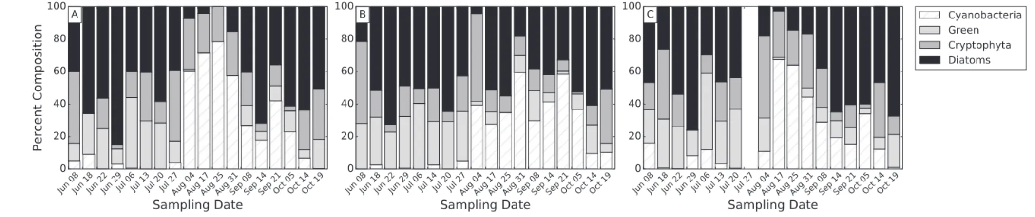
The phytoplankton community composition was relatively similar across stations as evidenced from sampling at three stations (Fig. 4). The percentage due to cyanobacteria increased at all stations during the cyanoHAB growing season (July 22–October 18). These time series also showed the varying contribution of diatoms over time. At stations WE2 and WE12 (Fig. 4A and C, respectively), the increase in cyanobacteria percentage appeared to coincide with a decrease in dia-tom percentage. At station WE6 (Fig. 4B), the diatoms maintained a strong contribution throughout the cyanoHAB growing season.

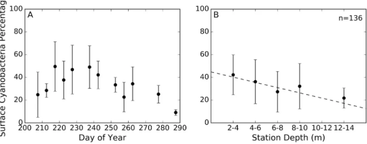
There was a significant increase in surface layer cyanobacteria con-tribution in the cyanoHAB growing season (p_b0.01; Wilcoxon Rank Sum test). The cyanobacteria contribution outside the cyanoHAB season was 6.1% and increased to 34.8% within the growing season. When narrowing to the cyanoHAB season there was a signi_ficant decline in cyanobacteria contribution as the season progressed (p b 0.01; Fig. 5A). Moreover, there was a significant decline in surface layer cyanobacteria contribution as water depth increased (pb0.01;Fig. 5B).

On average, the cyanobacteria were uniformly distributed through-out the water column during the study period. The mean cyanobacteria center of mass ranged from 0.25 to 0.64 during the cyanoHAB season with a mean of 0.48 which is effectively well-mixed. This indicates that in a hypothetical 10 m water column, the cyanobacteria concentra-tion would be centered at 4.8 m as opposed to 5 m in a perfectly well-mixed scenario with a center of mass of 0.5. There was a statistically sig-nificant (pb0.01) decrease in center of mass as the season progressed and a significant increase in center of mass as water depth increased (pb0.01).

Our data revealed a significant relationship between cyanobacteria center of mass and cyanobacteria concentration within the surface layer, such that increases in surface layer concentrations corresponded with decreases in the center of mass (pb0.01). Because of this observed relationship, we split our dataset into two categories based on surface layer cyanobacteria concentration in order to more clearly see how other variables (i.e., time, station depth, wind speed, and wave height) influence the vertical structure. The high concentration category in-cluded casts where the surface layer cyanobacteria concentration exceeded the mean (3.76μg/L,n= 65) and low concentration was de-fined as casts where the surface layer concentration was below the mean (n= 71).

The low concentration category exhibited a significant declining trend over time (pb0.01;Fig. 6A) but binning this data into 5 day inter-vals showed that the average center of massfluctuated around 0.5 with only two bins showing significant discrepancies from 0.5 based on the Wilcoxon Signed-Rank test (p= 0.027, 0.043 for the August 13–18 and August 28–September 2 bins, depicted as days 227 and 242, respec-tively). Both high and low cyanobacteria concentration data showed a significant decline in center of mass as station depth increased (pb

0.01;Fig. 6B). The 2-m binned low concentration data did not show any signi_ficant discrepancies from 0.5 throughout the depth range based on the Wilcoxon Signed-Rank test (allpN0.05). The binned high concentration data visually showed a clear decline in average cyanobacteria center of mass as depth increases and all bins had center of mass significantly lower than 0.5 (p= 0.045, 0.001, 0.028, 0.007 for the 2–4, 4–6, 6–8, and 8–10 m bins, respectively). Similarly, when looking only at deeper stations (those with depth greater than the over-all average of 6.2 m), there was a clear decline in center of mass as sur-face layer cyanobacteria concentrations increased (p b 0.01). In summary, cyanobacteria tended to be vertically stratified in deeper off-shore waters when surface layer concentrations were high, with strati-fication becoming more severe with increasing depths and/or increasing surface layer concentrations. Cyanobacteria were generally well-mixed in shallower nearshore waters and/or when surface layer cyanobacteria concentrations were low.

Projecting the surface layer concentration throughout the water col-umn allows for the assessment of biomass estimation error if one were

Fig. 2.Variability of Satlantic HyperPro-derived optical depths for all stations from July 22 through October 18 in 2015 and 2016. A) optical depth plotted against the sampling date, B) optical depth plotted against the station depth. For each date and station depth bin, the dot represents the mean optical depth and the bars represent one standard deviation.

483

to assume a well-mixed condition. When water depths wereb6.2 m and surface layer concentrations were high, assuming a well-mixed water column resulted in an average biomass overestimation of 6.7% and got as high as 52.1%. When water depths wereN6.2 m, the average biomass overestimation was 33.9% reaching as high as 75.3%.

In order to examine other factors controlling cyanobacteria vertical distribution we compared cyanobacteria distribution to wind speed and wave height. Because cyanobacteria were well-mixed when the surface layer concentration was low, modeled wind speed and wave height data were only compared to the cyanobacteria center of mass for casts when high surface layer concentrations were observed (Fig. 7). A segmented regression analysis (using the segmented package in R;Muggeo, 2008) showed that there was a significant shift in the re-lationships at a wind speed of 4.9 m per second (pb0.01) and a wave height of 0.27 m (p= 0.037). This analysis found significant positive slopes when wind speeds and wave heights were below the thresholds (slope = 0.07 andpb0.01 for wind speed, slope = 0.19,p= 0.014 for wave height) and non-significant slopes when wind speeds and wave heights were greater than the thresholds with center of mass values av-eraging 0.49 above the threshold in both comparisons. The piecewise regression model for wind speed explained more variability than the wave height model, with R2values of 33.7% and 26.7%, respectively. Comparing the segmented model R2_{using different aggregation times,}

it was found that averaging wind speeds and wave heights over the 24 h prior to sampling provided a betterfit than any of the shorter time periods.

Discussion

Remote sensing has been used to study cyanoHAB extent, severity, and movement in Lake Erie due to its spatial and temporal sampling ad-vantages overin situtracking (Wynne et al., 2008;Stumpf et al., 2012; Wynne et al., 2013;Sayers et al., 2016). There are key limitations with remote sensing though that could inhibit the ability to use the satellite retrievals to adequately monitor cyanoHAB events. Because satellites can only observe water down to one optical depth, assumptions have to be made about the vertical structure in order to make water column cyanobacteria biomass estimates. If the vertical structure is variable, then a universal assumption of either mixed or stratified would lead to errors in these estimates. Approaches that assume a highly stratified water column and treat the surface layer concentrations as the majority of the water column biomass (i.e.,Wynne et al., 2010;Stumpf et al., 2012) would underestimate in cases where the water column was more mixed. Conversely, approaches that assume a homogenous cyanobacteria distribution (asBertani et al., 2016did forin situ mea-surements) would overestimate biomass in cases where vertical strati-fication was present. This study used an extensivein situFP time series to investigate the variability of vertical structure in western Lake Erie in order to assess the ability of remote sensing to study cyanoHAB in west-ern Lake Erie.

Even though cyanobacteria were typically homogenously distrib-uted throughout the water column, significant variability was seen in the cyanobacteria vertical structure metric, particularly when cyanobacteria concentrations were high. When cyanobacteria concen-trations within the surface layer were elevated, the center of mass was found to be significantly lower than 0.5 (indicating that the cyanobacteria were more concentrated toward the air-water interface) and the vertical stratification became more severe as water depth in-creased. Cyanobacteria has been reported to be well-mixed in shallow lakes (Hunter et al., 2008), and stratification at increased depths is likely due to temperature gradients since cyanoHAB growth is sensitive to temperature (Robarts and Zohary, 1987;Kanoshina et al., 2003). Rowe reported that western Lake Erie experiences varying surface mixed layer depths as a result of the“diel cycle of surface heating and cooling” with additional influence from wind and that cyanobacteria buoyancy is able to keep concentrations within this surface mixed layer where growth conditions are optimal (Rowe et al., 2016).

The explanation for the relationship between cyanobacteria vertical structure and surface layer concentration is less clear. Given that the center of mass metric indicates where in the water column the cyanobacteria is most heavily concentrated and that cyanobacteria buoyancy limits the presence at depths below the surface mixed layer, it is intuitive that increased concentrations in the surface layer would skew the center of mass higher in the water column. However, it is also possible that increased concentrations of cyanobacteria in the sur-face layer are driving center of mass shifts in more indirect ways. It has been shown that cyanobacteria blooms can increase the water tem-perature near the air-water interface, providing a positive feedback mechanism leading to increased cyanobacteria presence (Hense, 2007). Additionally, in small lakes, increased concentrations of cyanobacteria are known to diminish the depth of the surface mixed layer by attenuating light (Mazumder et al., 1990;Fee et al., 1996; Houser, 2006), though this effect may be less of a factor in large lakes (Fee et al., 1996). A potential confounding factor here is that cyanobacteria colony size has been linked to increased buoyancy (Walsby, 1972;Reynolds et al., 1987) so it is possible that the observed relationship between cyanobacteria concentration and vertical struc-ture is the result of a spurious correlation between concentration and colony size. Going forward, collecting particle size distribution data along with the FP profiles (either through the use of anin situ instru-ment or a laboratory analysis of water samples) would allow for further unraveling of this relationship.

Wind speed and/or wave height were also found to be critical to de-termining periods when cyanobacteria may be vertically stratified in the water column. Heavy winds have been widely reported as a key driver of vertical mixing of cyanoHAB (Wallace et al., 2000;Gons et al., 2005;Hunter et al., 2008; Wynne et al., 2010;Rowe et al., 2016). Several studies have identified threshold wind speeds required for vertical mixing in shallow inland lakes, from 3.1 m/s (Cao et al., 2006) to 4 m/s (George and Edwards, 1976; Hunter et al., 2008; Fig. 3.Example FP profiles demonstrating different vertical structures in western Lake Erie and the corresponding cyanobacteria center of mass. A) example of a well-mixed station from WE13 on 8/25/2015 where the cyanobacteria center of mass is approximately 0.5, B) example of a vertically stratified cyanobacteria population from WE2 on 8/17/2015 with a cyanobacteria center of mass of approximately 0.33, C) example of a highly stratified cyanobacteria population from WE2 on 8/31/2015 with a center of mass of approximately 0.29.

Fig. 4.Surface layer algal composition time series for three stations in WBLE in 2015: WE2 (A), WE6 (B), and WE12 (C). Each bar represents the percent composition of total chlorophyll-aby each algal group over the top 1.12 m. Empty columns indicate dates where sampling occurred, but no FP measurements were recorded within the top 1.12 m.

48 5 K .R .Bo ss e et a l. / Jo u rn al of Gr ea t La k es Re se ar ch 4 5 (2 0 1 9 ) 48 0 – 48 9

Huang et al., 2014). A 6.2 cm wave height threshold, or approximately 0.2 ft, was previously identified as sufficient to force mixing (Cao et al., 2006). These thresholds are lower than what was identified in our analysis (4.9 m/s wind speeds and 0.91 ft wave heights), likely due to the fact that western Lake Erie is deeper than the other lakes studied. Wind mixing thresholds have also been identified using remote sensing for larger lakes more similar to Lake Erie. For Lake of the Woods (which straddles the USA/Canada border),Binding et al. (2011) re-ported a lower cyanobacteria mixing threshold at wind speeds of 3 m/s, though this was for blooms ofAphanizonmenonrather than Microcystis(Binding et al., 2011). StudyingMicrocystisblooms in west-ern Lake Erie,Wynne et al. (2010)found a greater threshold wind speed, reporting that wind speedsN15 knots (approximately 7.7 m/s) were likely to cause mixing. This study'sfinding of a threshold at 4.9 m/s most closely matches the NOAA Lake Erie Harmful Algal Bloom Bulletin, which notes that wind speedsN10 knots (approxi-mately 5.14 m/s) may result in an increased chance of mixing (https://tidesandcurrents.noaa.gov/hab/hab_publication/Lake_Erie_ HAB_Bulletin_Guide.pdf; accessed on July 20, 2018). Because the verti-cal structure varies with station depth as well as disturbance due to winds and waves, it follows that a universal assumption of either a mixed or stratified water column would lead to errors in estimating cyanobacteria biomass based on remote sensing-derived surface layer values.

Aside from varying water column vertical structure, current remote sensing algorithms also face issues with how cyanobacteria concentra-tions are derived. Due to spectral resolution limitaconcentra-tions of most sensors, these algorithms are typically using spectral features specific to chlorophyll-a (i.e., the chlorophyll-a absorption maxima around 667 nm, andfluorescence peak at 681 nm,etc.) to generate relationships to estimate cyanobacteria abundance/biomass (Wynne et al., 2010; Stumpf et al., 2012;Sayers et al., 2016). This approach is adequate if cyanobacteria are consistently the dominant algal group during the cyanoHAB season, but if the surface layer algal group composition is var-iable then these relationships could be invalid. Wynne notes that the CI algorithm“may be sensitive to large blooms of other types of phyto-plankton”(Wynne et al., 2010).

Western Lake Erie was found to exhibit a diverse phytoplankton community even during the cyanoHAB growing season. Despite the in-creased concentration of cyanobacteria during the bloom season, they only accounted forN50% of total chlorophyll-ain the surface layer in 17% of the samplings during bloom season. The mean cyanobacteria contribution during the bloom season was 34.8%, similar to what was reported in 2005 and greater than what was seen in 2003 and 2004 (Millie et al., 2009). Seasonal trends observed in the FP data were also compared to previously reported trends. Diatoms were the dominant algal group from the start of sampling until late July and again in the fall as the cyanobacteria died down, agreeing well with thefindings of Fig. 5.Temporal and spatial variability of surface layer cyanobacteria percentage for all stations from July 22 through October 18 in 2015 and 2016. A) cyanobacteria percent composition in the top 1.12 m plotted against the sampling date, B) cyanobacteria percent composition in the top 1.12 m plotted against the station depth. Regression line in panel B was calculated using the full un-binned dataset and was derived using the Theil-Sen Estimator, showing a significant decline in percent composition as depth increased (pb0.01). For each date and station depth bin, the dot represents the mean optical depth and the bars represent one standard deviation.

Fig. 6.Temporal and spatial variability of cyanobacteria center of mass for all stations from July 22 through October 18 in 2015 and 2016, with data split by surface layer cyanobacteria concentration. High concentration represents casts where the surface layer cyanobacteria concentration was greater than the mean (3.76μg/L) and low concentration represents casts where the surface layer concentration was below the mean. A) cyanobacteria center of mass plotted against the sampling date, B) cyanobacteria center of mass plotted against the station depth. Regression lines in panel B were calculated using the full un-binned dataset and were derived using the Theil-Sen Estimator, both showing a significant decline in center of mass as depth increased (pb0.01). For each date and station depth bin, the dot represents the mean optical depth and the bars represent one standard deviation.

priorin situstudies (Munawar and Munawar, 1982;Ghadouani and Smith, 2005). Cyanobacteria began developing in late-July in Maumee Bay before spreading eastward and persisted until mid-October, corre-sponding well with observations based on remote sensing (Wynne and Stumpf, 2015).

Our analysis also showed that the contribution of cyanobacteria to the total chlorophyll-aconcentration was found to be variable through time and space in western Lake Erie. Cyanobacteria contribution de-clined significantly over the cyanoHAB season, but this trend appears to be better modeled with a non-linear function. The percentage of cyanobacteria in the surface layer increases from the beginning of the growing season, peaking in mid-August before it begins to decline. Liter-ature suggests that the cyanobacteria peak varies by year (Bridgeman et al., 2013), but the mid-August peak we identified was also seen in other studies (Bridgeman et al., 2013;Wynne and Stumpf, 2015). Cyanobacteria were shown to be more dominant at shallow stations, with its contribution declining as station depth increased. Geographi-cally, the shallowest sampling stations are closest to the mouth of the Maumee River and depths increase as distance from Maumee Bay in-creases. Multiple remote sensing studies have shown that within west-ern Lake Erie, Maumee Bay is most severely impacted by cyanoHAB with maps showing declining severity further from the Maumee River (Wynne and Stumpf, 2015;Sayers et al., 2016). The variable phyto-plankton community and cyanobacteria contribution suggest that in most cases one cannot simply use chlorophyll-aconcentration as a sur-rogate for cyanobacteria abundance/biomass.

Since significant variability was identified in cyanobacteria vertical structure and surface layer composition, current remote sensing ap-proaches for tracking cyanobacteria may require some improvement when being used to estimate water column biomass. This could include expanding algorithms to utilize spectral features more specific to cyanobacteria in addition to the total chlorophyll-afeatures currently targeted, including the absorption maxima at 620 nm (Bryant, 1994) which is available on the European Space Agency's Ocean Land Color In-strument (OLCI) aboard Sentinel-3. Stumpf et al. note that the total chlorophyll-afeatures at 665 and 681 nm are targeted rather than the 620 nm band because of the increased sensitivity of these bands to pig-ment concentration which enhances the ability of satellite remote sens-ing algorithms to retrieve biomass variations (Stumpf et al., 2016). However, the maximum peak height (MPH) algorithm, while retrieving concentrations of chlorophyll-arather than cyanobacteria, uses these more sensitive bands while also incorporating the 620 nm band as an indicator of cyanobacteria presence (Matthews et al., 2012;Matthews and Odermatt, 2015). Promise has also been shown in the use of hyperspectral remote sensing to utilize these and other bands to track cyanobacteria blooms (Kudela et al., 2015) and to break down the ob-served water color into phytoplankton functional groups (Werdell

et al., 2014). Other indicators or predictors (i.e., water temperature) could also be used to help estimate cyanobacteria abundance/biomass from chlorophyll-ameasures (Stumpf et al., 2012;Sayers et al., 2016).

There has been little reporting on the variability of optical depth and light attenuation in Lake Erie.O'Donnell et al. (2010)measured the dif-fuse attenuation coefficient (Kd) at 14 stations in the western and

cen-tral basins of Lake Erie over the course of two days in 2007,finding large differences driven by the concentration and composition of opti-cally active constituents including chlorophyll-a. Based on the calcula-tion of optical depth as the inverse of Kd, they found spectrally

averaged optical depths ranging from approximately 0.66 to 1.66 m (O'Donnell et al., 2010). Results from this study showed an approxi-mately four-fold larger range of optical depths, likely because of our ex-panded temporal sampling. The exex-panded range of optical depths reported in this study is important for the interpretation of remote sens-ing data in terms of understandsens-ing the volume of water besens-ing observed by the sensors.

Knowledge of the spectral variability of optical depths is also impor-tant when using remote sensing to study water quality. An optical depth of approximately 1 m for the wavelengths between 660 and 700 nm had been previously estimated based on a chlorophyll concentration of 10

μg/L (Wynne et al., 2010). Our data was in agreement with this value, with an average optical depth of 0.9 m across the same wavelengths, however depths were found to range from 0.35 to the theoretical pure water maximum of 2 m (Pope and Fry, 1997;Wynne et al., 2010). The range of optical depths was much wider at other wavelengths which is critical information for algorithms utilizing other portions of the opti-cal spectrum. At the commonly used 550 nm band (O'Reilly et al., 2000; Shuchman et al., 2013) the average optical depth observed was 1.6 m but ranged between 0.3 and 9.3 m. This spectral variability indicates that remote sensing bands in different portions of the spectrum (i.e., red, green, and blue) are observing different volumes of water. In the case of a well-mixed water column, this effect is likely negligible. How-ever, under stratified conditions, these different volumes could contain different particle compositions and/or concentrations. The vertical dis-tribution of cyanobacteria has been shown to impact remote sensing re-flectance retrievals (Kutser et al., 2008), indicating that multispectral remote sensing algorithms for studying cyanoHAB need to take this varying optical depth into account.

The FP has been shown to be an effective tool to characterize phyto-plankton inin situsettings (Gregor and Maršálek, 2004;Ghadouani and Smith, 2005), but the application of FP results does require some cau-tion. Due to the FP deployment methods and outputfiltering of upcast data, there is limited sampling of the top meter of the water column. The average depth of thefirst measurement was 0.62 m below the air-water interface and 12.5% of casts did not have a measurement within 1 m of the air-water interface. Because cyanoHABs are known to Fig. 7.Comparison between cyanobacteria center of mass and modeled wind speed (A) and modeled significant wave height (B) for all points within the cyanoHAB growing season (July 22–October 18) in 2015 and 2016. The plotted lines represent the results from segmented regression analysis. Both wind speed and wave height showed a significant positive relationship with center of mass up to a threshold value, above which the water column was consistently well-mixed (wind speed: slope = 0.07,pb0.01, threshold = 4.9 m/s; wave height: slope = 0.19,p= 0.014, threshold = 0.27 m).

487

concentrate near the air-water interface in calm conditions, our FP dataset may have missed some of the largest concentrations of cyanobacteria, particularly when surface scums were present. The cyanobacteria dominance in the surface layer is likely underestimated by not sampling this shallowest portion of the water column. In highly strati_fied conditions, not sampling the top meter may also falsely sug-gest a more mixed water column than is actually present.

Undersampling the top meter of water does not invalidate the trends that were found, but it does compromise our ability to directly link the FP results to remote sensing retrievals. This is particularly true in turbid waters where the optical depth could be shallow enough that it is not sampled at all by current FP deployment methods. There are a few methodological improvements that can be made to the FP deployment to improve sampling within the top meter of water. For example, after allowing the FP to warm up in the water, the instrument can be lifted completely out of the water before beginning the descent process. Alter-natively, the FP can be deployed in a horizontal position. Since the instrument's LED sensors are located approximately 0.5 m below the top of the cage, a horizontal deployment would allow the user to ensure that the top portion of the water column is being sampled even if the warm up period takes place in the water. Increasing the sampling rate (slower rate of lowering) would also allow for more measurements within the top meter. Another approach to ensure data within the top meter would be to collect a water sample from the surface layer, store it in a cool, dark space, and analyze it in the lab with the FP in WorkSta-tion mode. Since surface scum thickness generally does not exceed 1–2 cm it is unlikely to ever be adequately sampled with a FP in the field. In this case, integration with remote sensing algorithms that iden-tify surface scums could be used to ideniden-tify areas where the well-mixed water column assumption is not met. One such algorithm is the Surface Scum Index (SSI) which uses an implementation of the NDVI over water pixels to identify scums (Sayers et al., 2016).

The FP is also susceptible to errors in pigmentfluorescence quantum yields which can vary in surface layer samples due to non-photochemical quenching (NPQ) (Falkowski and Raven, 2007). Quenching has been shown to increase as the level of incoming radia-tion increases (Sackmann et al., 2008), causing the FP to underestimate concentrations by 10–40% in waters where the photosynthetically ac-tive radiation is greatest (Leboulanger et al., 2002;Serra et al., 2009). Be-cause radiation levels decrease in deeper waters,fluorescence quantum yields can increase and lead to biased vertical profiles, suggesting a deep chlorophyll layer when one is not actually present (Sackmann et al., 2008).Microcystishas been suggested to be less impacted by NPQ than other species (Paerl et al., 1985;Sommaruga et al., 2009), but NPQ could lead to overestimates of cyanoHAB dominance in the surface layer while also limiting our ability to study the concentration and structure of other algal groups with FP data.

Several techniques exist for avoiding NPQ or correcting for it. In low-sediment waters, particulate backscattering has been shown to be cor-related with chlorophyll-aconcentrations and thefl uorescence:back-scattering ratio can be propagated from deep layers to the air-water interface to determine the level of quenching and correct for it (Sackmann et al., 2008). However, sediments are frequently present in western Lake Erie, limiting the effectiveness of this approach. Concur-rent photochemical yield estimations can also be used to correct for NPQ (Chekalyuk and Hafez, 2011). Sampling at night or before sunrise would limit the effect of NPQ on our data, but would also limit the appli-cability of the results to remote sensing data (most satellitesfly over be-tween 11 am and 2 pm) due to relatively rapid daily vertical migration patterns typically observed for buoyant cyanobacteria (Kromkamp and Mur, 1984;Ibelings et al., 1991).

Despite the minor issues with the data, this extensive FP dataset has provided and will continue to provide extreme value to the research community. The FP provides a quick way to assess vertical homogeneity of phytoplankton, a necessary requirement for applications to remote sensing. The spatial and temporal coverage of this dataset allows for

users of the data to study trends across the western basin over the course of multiple growing seasons at afiner scale than prior data allowed.

Acknowledgements

This work was supported by the National Oceanic and Atmospheric Administration Great Lakes Environmental Research Laboratory (NOAA GLERL) through the Cooperative Institute for Great Lakes Research (CIGLR) under subcontract #3004701270 and the National Aeronautics and Space Administration (NASA) under contract #80NSSC17K0712. The authors would like to thank the interns who assisted in processing data for this project, including: Ethan Ader, Anthony Chavez, Alice El-liott, and Jeremiah Harrington.

References

Ackerman, S.A., Heidinger, A., Foster, M.J., Maddux, B., 2013.Satellite regional cloud clima-tology over the Great Lakes. Remote Sens. 5 (12), 6223–6240.

Beeton, A.M., 1965.Eutrophication of the St. Lawrence great lakes. Limnol. Oceanogr. 10 (2), 240–254.

Bertani, I., Obenour, D.R., Steger, C.E., Stow, C.A., Gronewold, A.D., Scavia, D., 2016. Proba-bilistically assessing the role of nutrient loading in harmful algal bloom formation in western Lake Erie. J. Great Lakes Res. 42 (6), 1184–1192.

Beutler, M., Wiltshire, K.H., Meyer, B., Moldaenke, C., Lüring, C., Meyerhöfer, M., Hansen, U.P., Dau, H., 2002.Afluorometric method for the differentiation of algal populations in vivo and in situ. Photosynth. Res. 72 (1), 39–53.

Binding, C.E., Greenberg, T.A., Jerome, J.H., Bukata, R.P., Letourneau, G., 2011.An assess-ment of MERIS algal products during an intense bloom in Lake of the Woods. J. Plankton Res. 33 (5), 793–806.

Bridgeman, T.B., Chaffin, J.D., Filbrun, J.E., 2013.A novel method for tracking western Lake ErieMicrocystisblooms, 2002–2011. J. Great Lakes Res. 39 (1), 83–89.

Bryant, D.A. (Ed.), 1994.The Molecular Biology of Cyanobacteria. Kluwer Academic, Dor-drecht, The Netherlands.

Cao, H.S., Kong, F.X., Luo, L.C., Shi, X.L., Yang, Z., Zhang, X.F., Tao, Y., 2006.Effects of wind and wind-induced waves on vertical phytoplankton distribution and surface blooms of Microcystis aeruginosa in Lake Taihu. J. Freshw. Ecol. 21 (2), 231–238. Chekalyuk, A., Hafez, M., 2011.Photo-physiological variability in phytoplankton

chloro-phyllfluorescence and assessment of chlorophyll concentration. Opt. Express 19 (23), 22643–22658.

Conroy, J.D., Kane, D.D., Dolan, D.M., Edwards, W.J., Charlton, M.N., Culver, D.A., 2005. Temporal trends in Lake Erie plankton biomass: roles of external phosphorus loading and dreissenid mussels. J. Great Lakes Res. 31, 89–110.

Escoffier, N., Bernard, C., Hamlaoui, S., Groleau, A., Catherine, A., 2015.Quantifying phyto-plankton communities using spectralfluorescence: the effects of species composition and physiological state. J. Plankton Res. 37 (1), 233–247.

Falkowski, P.G., Raven, J.A., 2007.Aquatic Photosynthesis. Princeton University Press, Princeton, NJ.

Fee, E.J., Hecky, R.E., Kasian, S.E.M., Cruikshank, D.R., 1996.Effects of lake size, water clar-ity, and climatic variability on mixing depths in Canadian Shield lakes. Limnol. Oceanogr. 41 (5), 912–920.

Fernandes, R., Leblanc, S.G., 2005.Parametric (modified least squares) and non-parametric (Theil–Sen) linear regressions for predicting biophysical parameters in the presence of measurement errors. Remote Sens. Environ. 95 (3), 303–316. George, D.G., Edwards, R.W., 1976.The effect of wind on the distribution of chlorophyll a

and crustacean plankton in a shallow eutrophic reservoir. J. Appl. Ecol. 13, 667–690. Ghadouani, A., Smith, R.E., 2005.Phytoplankton distribution in Lake Erie as assessed by a

newin situspectrofluorometric technique. J. Great Lakes Res. 31, 154–167. Gons, H.J., Hakvoort, H., Peters, S.W., Simis, S.G., 2005.Optical detection of cyanobacterial

blooms. In: Huisman, J., Matthijs, H.C.P., Visser, P.M. (Eds.), Harmful Cyanobacteria. Springer, Netherlands, pp. 177–199.

Gordon, H.R., McCluney, W.R., 1975.Estimation of the depth of sunlight penetration in the sea for remote sensing. Appl. Opt. 14 (2), 413–416.

Gregor, J., Maršálek, B., 2004.Freshwater phytoplankton quantification by chlorophyll a: a comparative study of in vitro, in vivo, and in situ methods. Water Res. 38 (3), 517–522.

Heaney, S.I., Furnass, T.I., 1980.Laboratory models of diel vertical migration in the dinofl a-gellateCeratium hirundinella. Freshw. Biol. 10 (2), 163–170.

Henry, T., 2014. Toledo seeks return to normalcy after do not drink water advisory lifted. Toledo Blade (5 August) Available at.http://www.toledoblade.com/local/2014/08/ 05/Toledo-seeks-return-to-normalcy-after-do-not-drink-water-advisory-lifted.html. Hense, I., 2007.Regulative feedback mechanisms in cyanobacteria-driven systems: a

model study. Mar. Ecol. Prog. Ser. 339, 41–47.

Houser, J.N., 2006.Water color affects the stratification, surface temperature, heat con-tent, and mean epilimnetic irradiance of small lakes. Can. J. Fish. Aquat. Sci. 63 (11), 2447–2455.

Huang, C., Li, Y., Yang, H., Sun, D., Yu, Z., Zhang, Z., Chen, X., Xu, L., 2014.Detection of algal bloom and factors influencing its formation in Taihu Lake from 2000 to 2011 by MODIS. Environ. Earth Sci. 71 (8), 3705–3714.

Hunter, P.D., Tyler, A.N., Willby, N.J., Gilvear, D.J., 2008.The spatial dynamics of vertical migration byMicrocystis aeruginosain a eutrophic shallow lake: a case study using

high spatial resolution time-series airborne remote sensing. Limnol. Oceanogr. 53 (6), 2391–2406.

Ibelings, B.W., Mur, L.R., Walsby, A.E., 1991.Diurnal changes in buoyancy and vertical dis-tribution in populations ofMicrocystisin two shallow lakes. J. Plankton Res. 13 (2), 419–436.

International Joint Commission (IJC), 2014.A Balanced Diet for Lake Erie: Reducing Phos-phorus Loadings and Harmful Algal Blooms.

Kanoshina, I., Lips, U., Leppänen, J.M., 2003.The influence of weather conditions (temper-ature and wind) on cyanobacterial bloom development in the Gulf of Finland (Baltic Sea). Harmful Algae 2 (1), 29–41.

Komsta, L., 2013.mblm: Median-Based Linear Models. R Package Version 0.12. Kromkamp, J.C., Mur, L.R., 1984.Buoyant density changes in the cyanobacterium

Microcystis aeruginosadue to changes in the cellular carbohydrate content. FEMS Microbiol. Lett. 25 (1), 105–109.

Kudela, R.M., Palacios, S.L., Austerberry, D.C., Accorsi, E.K., Guild, L.S., Torres-Perez, J., 2015. Application of hyperspectral remote sensing to cyanobacterial blooms in inland wa-ters. Remote Sens. Environ. 167, 196–205.

Kutser, T., Metsamaa, L., Dekker, A.G., 2008.Influence of the vertical distribution of cyanobacteria in the water column on the remote sensing signal. Estuar. Coast. Shelf Sci. 78 (4), 649–654.

Lake Erie Lamp, 2011.Lake Erie Binational Nutrient Management Strategy: Protecting Lake Erie by Managing Phosphorus (Prepared by the Lake Erie LaMP Work Group Nu-trient Management Task Group).

Leboulanger, C., Dorigo, U., Jacquet, S., Le Berre, B., Paolini, G., Humbert, J.F., 2002. Appli-cation of a submersible spectrofluorometer for rapid monitoring of freshwater cyanobacterial blooms: a case study. Aquat. Microb. Ecol. 30 (1), 83–89.

Lee, Z., Shang, S., Du, K., Wei, J., 2018. Resolving the long-standing puzzles about the ob-served Secchi depth relationships. Limnol. Oceanogr.https://doi.org/10.1002/ lno.10940.

Makarewicz, J.C., 1993.Phytoplankton biomass and species composition in Lake Erie, 1970 to 1987. J. Great Lakes Res. 19 (2), 258–274.

Matthews, M.W., Odermatt, D., 2015.Improved algorithm for routine monitoring of cyanobacteria and eutrophication in inland and near-coastal waters. Remote Sens. Environ. 156, 374–382.

Matthews, M.W., Bernard, S., Robertson, L., 2012.An algorithm for detecting trophic sta-tus (chlorophyll-a), cyanobacterial-dominance, surface scums andfloating vegetation in inland and coastal waters. Remote Sens. Environ. 124, 637–652.

Mazumder, A., Taylor, W.D., McQueen, D.J., Lean, D.R.S., 1990.Effects offish and plankton and lake temperature and mixing depth. Science. 247 (4940), 312–315.

Millie, D.F., Fahnenstiel, G.L., Bressie, J.D., Pigg, R.J., Rediske, R.R., Klarer, D.M., Tester, P.A., Litaker, R.W., 2009.Late-summer phytoplankton in western Lake Erie (Laurentian Great Lakes): bloom distributions, toxicity, and environmental influences. Aquat. Ecol. 43 (4), 915–934.

Montero, O., Sobrino, C., Parés, G., Lubián, L.M., 2002.Photoinhibition and recovery after selective short-term exposure to solar radiation offive chlorophyll c-containing ma-rine microalgae. Cienc. Mar. 28 (3), 223–236.

Muggeo, V.M., 2008.segmented: an R package tofit regression models with broken-line relationships. R news 8 (1), 20–25.

Munawar, M., Munawar, I.F., 1982.Phycological studies in Lakes Ontario, Erie, Huron, and Superior. Can. J. Bot. 60 (9), 1837–1858.

National Geophysical Data Center, 1999. Bathymetry of Lake Erie and Lake Saint Clair. https://doi.org/10.7289/V5KS6PHK.

Obenour, D.R., Gronewold, A.D., Stow, C.A., Scavia, D., 2014.Using a Bayesian hierarchical model to improve Lake Erie cyanobacteria bloom forecasts. Water Resour. Res. 50 (10), 7847–7860.

O'Donnell, D.M., Effler, S.W., Strait, C.M., Leshkevich, G.A., 2010.Optical characterizations and pursuit of optical closure for the western basin of Lake Erie through in situ mea-surements. J. Great Lakes Res. 36 (4), 736–746.

O'Reilly, J.E., Maritorena, S., Siegel, D.A., O'Brien, M.C., Toole, D., Mitchell, B.G., Kahru, M., Chavez, F.P., Strutton, P., Cota, G.F., Hooker, S.B., McClain, C.R., Carder, K.L., Muller-Karger, F., Harding, L., Magnuson, A., Phinney, D., Moore, G.F., Aiken, J., Arrigo, K.R., Letelier, R., Culver, M., 2000.Ocean Color Chlorophyll a Algorithms for SeaWiFS, OC2, and OC4: Version 4. SeaWiFS Postlaunch Calibration and Validation Analyses, Part, 3. pp. 9–23.

Paerl, H.W., 1983.Partitioning of CO2fixation in the colonial cyanobacteriumMicrocystis aeruginosa: mechanism promoting formation of surface scums. Appl. Environ. Microbiol. 46 (1), 252–259.

Paerl, H.W., Bland, P.T., Bowles, N.D., Haibach, M.E., 1985.Adaptation to high-intensity, low-wavelength light among surface blooms of the cyanobacteriumMicrocystis aeruginosa. Appl. Environ. Microbiol. 49 (5), 1046–1052.

Pope, R.M., Fry, E.S., 1997.Absorption spectrum (380–700 nm) of pure water. II. Integrat-ing cavity measurements. Appl. Opt. 36 (33), 8710–8723.

Reynolds, C.S., Oliver, R.L., Walsby, A.E., 1987.Cyanobacterial dominance: the role of buoyancy regulation in dynamic lake environments. N. Z. J. Mar. Freshw. Res. 21 (3), 379–390.

Rinta-Kanto, J.M., Konopko, E.A., DeBruyn, J.M., Bourbonniere, R.A., Boyer, G.L., Wilhelm, S.W., 2009.Lake ErieMicrocystis: relationship between microcystin production, dy-namics of genotypes and environmental parameters in a large lake. Harmful Algae 8 (5), 665–673.

Robarts, R.D., Zohary, T., 1987.Temperature effects on photosynthetic capacity, respira-tion, and growth rates of bloom-forming cyanobacteria. N. Z. J. Mar. Freshw. Res. 21 (3), 391–399.

Rowe, M.D., Anderson, E.J., Wynne, T.T., Stumpf, R.P., Fanslow, D.L., Kijanka, K., Vanderploeg, H.A., Strickler, J.R., Davis, T.W., 2016.Vertical distribution of buoyant Microcystisblooms in a Lagrangian particle tracking model for short-term forecasts in Lake Erie. J. Geophys. Res. Oceans 121 (7), 5296–5314.

Sackmann, B.S., Perry, M.J., Eriksen, C.C., 2008.Seaglider observations of variability in day-timefluorescence quenching of chlorophyll-a in Northeastern Pacific coastal waters. Biogeosci. Discuss. 5 (4), 2839–2865.

Sayers, M., Fahnenstiel, G.L., Shuchman, R.A., Whitley, M., 2016.Cyanobacteria blooms in three eutrophic basins of the Great Lakes: a comparative analysis using satellite re-mote sensing. Int. J. Rere-mote Sens. 37 (17), 4148–4171.

Schwab, D.J., Bedford, K.W., 1999.The great lakes forecasting system. Coast. Estuar. Stud. 157–173.

Sen, P.K., 1968.Estimates of the regression coefficient based on Kendall's tau. J. Am. Stat. Assoc. 63 (324), 1379–1389.

Serra, T., Borrego, C., Quintana, X., Calderer, L., López, R., Colomer, J., 2009.Quantification of the effect of nonphotochemical quenching on the determination of in vivo chl a from phytoplankton along the water column of a freshwater reservoir. Photochem. Photobiol. 85 (1), 321–331.

Shuchman, R.A., Leshkevich, G., Sayers, M.J., Johengen, T.H., Brooks, C.N., Pozdnyakov, D., 2013.An algorithm to retrieve chlorophyll, dissolved organic carbon, and suspended minerals from Great Lakes satellite data. J. Great Lakes Res. 39, 14–33.

Sommaruga, R., Chen, Y., Liu, Z., 2009.Multiple strategies of bloom-formingMicrocystisto minimize damage by solar ultraviolet radiation in surface waters. Microb. Ecol. 57 (4), 667–674.

Stumpf, R.P., Wynne, T.T., Baker, D.B., Fahnenstiel, G.L., 2012.Interannual variability of cyanobacterial blooms in Lake Erie. PLoS One 7 (8), e42444.

Stumpf, R.P., Davis, T.W., Wynne, T.T., Graham, J.L., Loftin, K.A., Johengen, T.H., Gossiaux, D., Palladino, D., Burtner, A., 2016.Challenges for mapping cyanotoxin patterns from remote sensing of cyanobacteria. Harmful Algae 54, 160–173.

Theil, H., 1950.A rank-invariant method of linear and polynomial regression analysis, part 3. Proceedings of Koninalijke Nederlandse Akademie van Weinenschatpen A. vol. 53, pp. 1397–1412.

Wallace, B.B., Bailey, M.C., Hamilton, D.P., 2000.Simulation of vertical position of buoy-ancy regulatingMicrocystis aeruginosain a shallow eutrophic lake. Aquat. Sci. 62 (4), 320–333.

Walsby, A.E., 1972.Structure and function of gas vacuoles. Bacteriol. Rev. 36 (1), 1. Werdell, P.J., Bailey, S.W., 2005.An improved in-situ bio-optical data set for ocean color

algorithm development and satellite data product validation. Remote Sens. Environ. 98 (1), 122–140.

Werdell, P.J., Roesler, C.S., Goes, J.I., 2014.Discrimination of phytoplankton functional groups using an ocean reflectance inversion model. Appl. Opt. 53 (22), 4833–4849. Wynne, T.T., Stumpf, R.P., 2015.Spatial and temporal patterns in the seasonal distribution

of toxic cyanobacteria in Western Lake Erie from 2002–2014. Toxins 7 (5), 1649–1663.

Wynne, T.T., Stumpf, R.P., Tomlinson, M.C., Warner, R.A., Tester, P.A., Dyble, J., Fahnenstiel, G.L., 2008.Relating spectral shape to cyanobacterial blooms in the Laurentian Great Lakes. Int. J. Remote Sens. 29 (12), 3665–3672.

Wynne, T.T., Stumpf, R.P., Tomlinson, M.C., Dyble, J., 2010.Characterizing a cyanobacterial bloom in western Lake Erie using satellite imagery and meteorological data. Limnol. Oceanogr. 55 (5), 2025–2036.

Wynne, T.T., Stumpf, R.P., Briggs, T.O., 2013.Comparing MODIS and MERIS spectral shapes for cyanobacterial bloom detection. Int. J. Remote Sens. 34 (19), 6668–6678. Xue, P., Schwab, D.J., Sawtell, R.W., Sayers, M.J., Shuchman, R.A., Fahnenstiel, G.L., 2017.A

particle-tracking technique for spatial and temporal interpolation of satellite images applied to Lake Superior chlorophyll measurements. J. Great Lakes Res. 43 (3), 1–13. 489