DRAFT FLARE WASTE GAS FLOW RATE AND COMPOSITION
MEASUREMENT METHODOLOGIES EVALUATION DOCUMENT
Prepared By:
Shell Global Solutions Shell Global Solutions (US) Inc.
3333 Highway 6 South Houston, Texas 77082
Lee K. Gilmer - Principal Investigator Christopher A. Caico
Jacob J. Sherrick Gary R. Mueller
TABLE OF CONTENTS
Page Executive Summary...E-1 1.0 INTRODUCTION... 1-1
1.3 Typical Flare Header/Tip Sizes ... 1-4 1.4 Typical Operating Conditions... 1-4 1.5 Typical Flow Rates/Ranges ... 1-4 1.5.1 Typical Velocity Ranges in Flare Systems... 1-5 1.5.2 NSPS J Flow Rate Limitations... 1-5 1.6 Typical Ranges/Variability of Waste Gas Composition... 1-6 1.7 Inherent flow meter precision and accuracy ... 1-9 1.8 Secondary selection criteria ... 1-10 1.9 Summary ... 1-10 2.0 FLARE WASTE GAS FLOW MEASUREMENT... 2-1
2.1 Flow Measurement Fundamentals ... 2-1 2.2 Flow Meter Evaluations... 2-1 2.2.1 Pitot Tubes... 2-4 2.2.2 Thermal Mass Meters... 2-8
2.2.3 Ultrasonic Time-of-Flight Meters... 2-13 2.2.4 Combination Systems ... 2-18
2.3 Factors Influencing Measurement Performance ... 2-19
2.3.1 Measurement Uncertainties ... 2-19 2.3.2 Combination Systems ... 2-22
2.4 Summary Overall Results of Flow Meter Evaluation... 2-33 3.0 FLARE WASTE GAS COMPOSITION MEASUREMENT... 3-1
3.1 Fundamentals ... 3-1 3.2 Analytical Performance Criteria Applicable to Flare Systems ... 3-1
3.2.1 Representative Sampling... 3-1 3.2.2 Constituentsof Interest ... 3-1
3.2.3 Dynamic Range ... 3-2 3.2.4 Separation... 3-3 3.2.5 Quantification... 3-3
3.3 Basics of Analytical Instrumentation Applicable to Flare Systems... 3-4
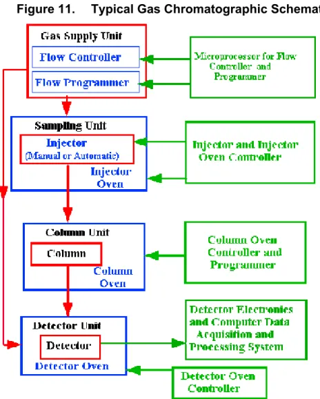
3.3.1 Gas-Solid Chromatography ... 3-4 3.3.2 Non Dispersive Infrared (NDIR) ... 3-5
3.3.3 Photoacoustic Sensor ... 3-6 3.4 Offline Techniques for Measurement of Flare Gas Compositions ... 3-8
3.4.1 EPA Method 18 ... 3-8 3.4.2 ASTM D-1945 and D-1946 ... 3-10 3.4.3 GPA 2261 and 2177... 3-12 3.4.4 Multichannel Micro GCs... 3-14 3.4.5 Summary of Offline Methods ... 3-19 3.5 Online Techniques for Measurement of Flare Gas Compositions... 3-20 3.5.1 Total VOC Analyzers ... 3-23
3.5.2 NDIR Analyzers ... 3-23 3.5.3 Permanent Online Monitoring Gas Chromatographs... 3-27
3.5.4 Permanent Online Monitors: Commercially Available Systems... 3-28
3.5.5 Photoacoustic Spectroscopy ... 3-32 3.5.6 Summary of Online Methods... 3-33
4.0 FLARE GAS EMISSION CALCULATION ERROR ANALYSIS... 4-1 4.1 Overall Error in Calculated Emissions ... 4-1 5.0 CONTROL OF GAS ASSIST RATIO ON OPERATING FLARES... 5-1
5.1 Introduction... 5-1 5.2 Examples of Assist Gas Ratio Control Techniques ... 5-2 5.3 Assist Gas Ratio Technique Performance... 5-4 5.4 Summary Results of Assist Gas Control Techniques Evaluation... 5-5 5.5 Developmental Recommendations ... 5-6 6.0 CONCLUSIONS AND RECOMMENDATIONS... 6-1 7.0 REFERENCES... 7-1 8.0 BIBLIOGRAPHY... 8-1
LIST OF FIGURES
Page
Figure 1. Elevated Flare 1-3
Figure 2. John Zink Thermal Oxidizer Flare “Ground Flare” 1-3 Figure 3. Range of Observed Waste Gas Velocities in Flare Systems 1-6
Figure 4. Molecular Weight Variations of Waste Gas 1-7 Figure 5. Generic Model of Pitot Tube 2-5 Figure 6. Generic Example of Thermal Mass Flow Meter 2-10 Figure 7. Comparison of Various Flow Measurement Techniques 2-13 Figure 8. Generic Example of Ultrasonic Flow Meter 2-14 Figure 9. Example Gas Flow Meter Calibration Curve 2-26 Figure 10. Effect of Averaging Time on Measured Flows 2-33 Figure 11. Typical Gas Chromatographic Schematic 3-5 Figure 12. Non-Dispersive Infrared Gas Analyzer 3-6 Figure 13. The Principal Components of a PAS Detector 3-7 Figure 14. Effect of Assist Gas on Combustion Efficiency 5-7 Figure 15. Influence on Steam on Global Efficiency 5-8 Figure 16. Manual Assist Gas Ratio Control Example 5-9 Figure 17. Automated Assist Gas Ratio Control Example 5-9 Figure 18. Smoke Monitor Assist Gas Ratio Control Example 5-10
LIST OF TABLES
Page
Table 1. Flare Waste Gas Compositions – Constituents and Variability 1-9 Table 2. Flow Meter Selection Table 2-3 Table 3. Typical Micro GC Configuration 3-15 Table 4. Summary of Offline Waste Gas Composition Measurement Techniques 3-17 Table 5. Online Non-Speciated Waste Gas Composition Measurement Techniques
Evaluation 3-21
Table 6. Online Speciated Waste Gas Composition Measurement Techniques Evaluation 3-25 Table 7. Emerging Waste Gas Composition Measurement Techniques 3-35
Executive Summary
The Texas Commission on Environmental Quality (TCEQ) has determined that Volatile Organic Compound (VOC) emissions may be underestimated in air shed emission inventories. It is expected that emissions from flares would be better estimated if they were based on waste gas flow rate and composition measurements. The TCEQ has established data quality objectives for conducting such measurements. This study evaluates currently available flow measurement and gas composition measurement techniques; their applicability to the measurement of waste gas flow and composition in flare systems and their ability to meet the data quality objectives established by TCEQ. Additionally, this study evaluates current practices for controlling assist gas to waste gas ratios in flares.
The overall objective of the Texas Commission on Environmental Quality (TCEQ) studies on flare emissions is to obtain performance specifications that ensure quality assured sampling, testing, monitoring, measurement, and monitoring systems for waste gas flow rate, waste gas composition, and assist gas flow rate. Specific objectives of this report are shown below.
To evaluate existing methods of monitoring or measuring waste gas flow rate and composition to determine the mass rate of volatile organic compounds (VOC) being routed to the flare within a known certainty. The overall desired accuracy, precision, and sensitivity is + 20 percent. Specifically for flow rate, composition measurements and the resulting calculated mass rate to the flare the desired accuracy, precision and sensitivity is + 20% (never to exceed + 5000 lb/hr) of total VOC emitted from the flare, whichever is greater. An additional consideration is the desire that the waste gas composition measurement methods must be able to provide 90% speciation by mass of the individual VOC in the waste gas with specific focus on propylene, ethylene, formaldehyde, acetaldehyde, isoprene, all the butenes/butylenes, 1,3-butadiene, toluene, all pentenes, all trimethylbenzenes, all xylenes, and all ethyltoluenes.
To evaluate methods of controlling the assist gas (steam or air) to waste gas ratio to assure the proper ratio is maintained within a known certainty. The overall desired accuracy, precision, and sensitivity is + 20 percent.
Flare systems are typically designed to burn large quantities of gas resulting from de-inventorying process units during emergencies. However, frequently they are also used to dispose of smaller quantities of waste gas, which are uneconomical to recover for beneficial use or as fuel. This dual mode of operation results in typical flows that are quite low, but sporadic high flow events. By design the number of compounds of interest and the dynamic range of these compounds can be quite large and variable. As a result of a detailed review of operating data from over 40 flares systems, current flow measurement techniques, and gas composition measurement techniques the following conclusions and recommendations have been developed. Waste Gas Flow Measurement Range
Due to the unique requirements of flare systems (low pressures, large pipe sizes, and 1000:1 turndown on flows) only multi-ranged pitot tubes, thermal mass meters, and ultrasonic time-of-flight meters are broadly applicable to the measurement of flows in flare systems.
Ultrasonic time-of-flight meters and Thermal mass meters can measure a greater range of gas velocities, and therefore are easier to apply to flare systems than pitot tubes. For the flares examined, all flows were below velocities of 300 fps, the high end measurable by ultrasonic and thermal mass meters. However, many flares are designed for worst-case events that will exceed this measurement capability.
Flow measurement systems that combine multiple measurement techniques can measure this design worst case. Using multiple measurement techniques increases the costs associated with purchase, installation, calibration, and maintenance of dual meters. Design worst-case events are infrequent and rarely occur. Typically, design worst-case events are associated with emergency, unplanned shutdowns of a complete process unit or the shutdown of several process units serving a flare due to a power failure. Other process data usually exist which can be used to estimate the mass flow during such events. Thus, the additional expense of installing multiple measurement systems may not be warranted due to the relative infrequency of such events and the availability of process data that can be used to estimate mass flow during worst-case design events.
Effects of Waste Gas Composition on Flow Measurements
Ultrasonic time-of-flight meters have greater accuracy and precision for measuring flows in flare gas systems, because they are less sensitive to changes in gas composition and can correct for variable gas composition using only flow meter inputs. Thermal mass meters and pitot tubes
need significant correction for changing gas compositions. Currently, real time correction for gas composition changes has not been demonstrated in field applications with thermal mass meters or pitot tubes, although vendors claim such meters are available. Correcting with periodic composition data adds to the uncertainty of the flow measurement of thermal mass meters and pitot tubes used in flare applications. Measurement of flows in flare systems can be made with an uncertainty in the range of + 5-10 percent. However, obtaining this accuracy in flare systems with highly variable compositions or where the meter cannot be located in a section of pipe with a representative flow profile will be a challenge.
Overall Flow Measurement Assessment
Currently, ultrasonic time of flight meters show the most promise of meeting the stated data quality objectives of this study in waste gas service. However, their cost probably limits their application to flow measurements at the terminal end of flare systems . Thermal mass meters offer a suitable alternative in services where the waste gas composition does not vary greatly, and as a sturdy portable instrument that can be used to troubleshoot flare systems (e.g. identify stray flows in complex flare headers).
Flare Waste Gas Composition Measurement
Measurement of the gas composition in flare systems on a continuous basis will be a challenge due to the number of compounds of interest and the dynamic range of concentrations, that may be present for the compounds of interest.
To design and implement a continuous monitoring system capable of detecting the full range of compounds of interest across all concentrations of interest using conventional GCs will require considerable up-front data collection, and fairly sophisticated combinations of columns and detectors.
If aldehydes happen to be present at quantities that would impact achieving the data quality objectives, the GC system required to analyze for them will become even more complex.
Portable multi-channel, micro GCs have proven extremely capable of detecting most compounds of interest in flare systems across an extremely large dynamic range (105). Application of such instruments in online applications will significantly reduce the complexity of the GC
instrumentation needed to achieve the data quality objectives of this study. However, online versions of these instruments have yet to be demonstrated in flare applications. While online GC
systems can be designed to meet the data quality objectives of this study a high percentage of the time, the actual percent of time the data quality objectives can be met will be a strong function of the specific flare system, in particular the variability of the waste gas composition. There is insufficient data available to make a fact-based estimate on this percentage.
Application of US EPA Performance Specification 9 to online GCs in flare service is problematic given the potential number of compounds of interest and the dynamic range potentially encountered for these compounds. The linearity requirement will be extremely difficult to meet and the calibration procedures impractical.
Picking a few representative compounds with which to calibrate and using relative response factors for other compounds of interest seems a practical solution. Due to the large dynamic range, the linearity requirement of PS9 may need to be relaxed in favor of a multipoint calibration curve.
Assist Gas Rate
Automatic controlling of the assist gas to waste gas ratio based on waste gas flow to the flare appears to be more effective at controlling this parameter at a desired value than manual control, but there was very little data available from which to make this conclusion. Additional data collection on the effectiveness of manual control would be warranted.
Waste Gas Flow and Composition Measurement Data Quality
The author’s assessment is that current flow and measurement technologies are capable of meeting the stated data quality objectives a high percentage of the time in most flares
applications. However, the scarcity of data on real world applications and the high degree of variability in flare applications make it impossible to quantify what percentage of the time these data quality objectives can be met, and on what percent of flare systems they may be met. Both flow and gas composition measurement vendors have responded to the added interest in
measurement of waste gas flow and composition. Significant recent developments have been made in both flow and composition measurement techniques. Demonstration of these
advancements could significantly enhance the ability of sources to meet these data quality objectives over a wider range of operations in the near future.
Under ideal conditions the mass flow in flare systems can be measured with an uncertainty in the + 5-10% range. However, problematic applications with widely varying gas compositions and poor meter installation geometries will have difficulty meeting the + 20% data quality objectives of this study.
Obtaining measurement of flare emissions within an absolute uncertainty of + 5,000 lb/hr
appears doable for all but the very largest flare. However, this assessment is strongly influenced by the 98% destruction efficiency assumption used in this study.
1.0 INTRODUCTION
The Texas Commission on Environmental Quality (TCEQ) has determined that flares may be a significant source of emissions of volatile organic compounds (VOC). Of particular interest are highly reactive volatile organic compounds (HRVOC), which may contribute to rapid ozone formation under certain atmospheric conditions. TCEQ is concerned that flare emissions may be one source of VOC and HRVOC emissions that are being underestimated in current air emission inventories and wants to investigate methods to improve emission estimates from this source. This study evaluates current flow measurement and gas composition measurement technologies, and their applicability to measuring waste gas flows and compositions to flares. In the past, other than requiring pilot lights to be monitored and lit at all times as well as limiting flare tip exit velocities and flare waste gas heating values, flares have not been subject to environmental regulations mandating accurate measurement of waste gas flows and compositions. Typically, flare waste gas flow rate and compositional measurements have been used to assist in designing flare gas recovery compressors, to identify sources upstream of the flare contributing to flare flows, to quantify the change in flare waste gas flow rates and compositions associated with process changes upstream of the flare header, and to assess normal flows versus design flows. The level of accuracy required for these purposes is not as stringent as that associated with regulatory requirements. Thus, existing instruments for measuring flare waste gas flows and compositions were not designed to meet stringent regulatory requirements.
TCEQ has established preliminary data quality objectives for measurements of waste gas flows to flares and wants to assess the ability of current technology to obtain these objectives. Further, as assist gas addition to flares is a primary means of improving combustion efficiency in flares at high load conditions, the TCEQ would like to evaluate methods used to control assist gas
addition to flares, and assess the ability of these methods to control the assist gas ratio within known certainties. This study assesses the ability of three common methods to control the assist gas to waste gas ratio.
1.1 Objectives
The overall objective of the TCEQ studies on flare emissions is to obtain performance specifications that ensure quality assured sampling, testing, monitoring, measurement, and monitoring systems for waste gas flow rate, waste gas composition, and assist gas flow rate. The
purpose of this project is to provide data and methodologies to improve emission estimates from flares. Specific objectives of this report are:
To evaluate existing methods of monitoring or measuring waste gas flow rate and composition to determine the mass rate of volatile organic compounds (VOC) being routed to the flare within a known certainty. The overall desired accuracy, precision, and sensitivity is + 20 percent. Specifically for flow rate, composition measurements and the resulting calculated mass rate to the flare the desired accuracy, precision and sensitivity is + 20% (never to exceed + 5000 lb/hr) of total VOC emitted from the flare, whichever is greater. An additional consideration is the desire that the waste gas composition measurement methods must be able to provide 90% speciation by mass of the individual VOC in the waste gas with specific focus on propylene, ethylene, formaldehyde, acetaldehyde, isoprene, all the butenes/butylenes, 1,3-butadiene, toluene, all pentenes, all trimethylbenzenes, all xylenes, and all ethyltoluenes.
To evaluate methods of controlling the assist gas (steam or air) to waste gas ratio to assure the proper ratio is maintained within a known certainty. The overall desired accuracy, precision, and sensitivity is + 20 percent.
1.2 Flare System Design and Operations 1.2.1 Purpose
Process flares are used as safety devices to combust large quantities of waste gases during emergency conditions, such as power failures or process upsets. Additionally, many facilities routinely flare smaller quantities of hydrocarbon gases that are exhausted at pressures too low to allow them to be routed to the facility fuel gas system or hydrocarbon gases that are
uneconomical to recover. Smaller ground flares are sometimes used to handle the smaller, more routine flows while higher capacity elevated flares are used for emergency condition flaring. Ground flares are designed for lower flow rates than elevated flares and typically the burners are enclosed in a stack. Also, their design (in the case of thermal oxidizers such as the one shown in Figure 2) results in a wider, less elevated, less visible, and less noisy flame. In simple terms, a thermal oxidizer ground flare flame is similar to a burner on a gas stove (several small flames from several points on a circle) while a traditional elevated flare flame is similar to a lit match (a larger, more defined flame emitted from a point). Figure(s) 1 and 2 provide schematics of typical ground and elevated flare systems.
1.2.2 Schematics
Figure 1. Elevated Flare1
Figure 2. John Zink Thermal Oxidizer Flare “Ground Flare” 2
1 Figure 1 is courtesy of John Zink Company. 2 Figure 2 is courtesy of John Zink Company.
1.3 Typical Flare Header/Tip Sizes
The authors have worked with or knowledge of the design and operation of approximately 40 flare systems in numerous U.S. refineries and chemical plants. The range in size of the terminal flare header, just prior to the flare, in these flare systems is from 24 to 60 inches in diameter with about 75% having a terminal diameter in the 36 to 48 inch range. Flare tip diameters utilized in these 40 flares range from 24 to 36 inches with over 80% in the 30 to 36 inch range. Therefore, to be broadly applicable flare waste gas flow measurement devices should be capable of being applied in line sizes from 4” up to 72”.
1.4 Typical Operating Conditions
The operating temperature in flare headers is typically at or very near ambient temperature due to the long lengths of pipe from the process unit boundary to the flare. Flare headers normally operate at very low pressures, typically at 1 to 2 psig. Some upstream relief valves relieve at pressures as low as 5 psig, necessitating the flare header operating pressure be designed as low as possible to insure flow from all required process relief systems to the flare system. The low operating pressures of most flare systems requires that a maximum pressure drop specification across any potential flare waste gas flow measurement device be set at less than 0.5 psig. Assist gas (usually steam or air) may be routed to the flare flame at the flare tip to assist mixing of combustion air, minimize smoking, and to maximize combustion efficiency. Since assist gas is added at the flare tip or into the flare riser, this gas will have no impact on the measurement of waste gas flows and compositions to the flare.
1.5 Typical Flow Rates/Ranges
Flare waste gas flows can range from nominally small flow rates of a few standard cubic feet per hour (SCFH) to several million SCFH. The U.S. EPA New Source Performance Standard for Flares (40CFR60.18) limits the maximum tip velocity for all flares constructed since 1973 to 400 feet per second, if the flare gas has a BTU content of at least 1,000 BTU/SCF and 60 feet per second for flares combusting gas with a BTU content of 300-1000 BTU/SCF. For the tip and header sizes in the flare systems the authors have worked with this velocity limitation equates to a maximum allowable volumetric flow rate of 4.5 million to 10 million SCFH or 100 to over 240
million standard cubic feet per day (for 24-36” flare tips). The authors’ discussions with
knowledgeable individuals from other companies would indicate that the above flow rate ranges are representative of flares at many of the petrochemical facilities in the Houston-Galveston airshed.
1.5.1 Typical Velocity Ranges in Flare Systems
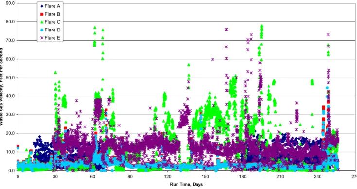
Most flow measurement devices that will be applicable to flare systems work on the principle of sensing the velocity of the waste gas stream, which is then converted into a volumetric or mass flow measurement. The large difference in flows between design maximums and normal operating flows for most flare systems leads to a requirement that any flow measurement device applied in flare systems to be capable of sensing a wide range of velocities. While there is no such thing as a typical flare system, hourly average data from 5 flares were examined over an eight-month period to demonstrate the range of velocities encountered in flare systems. These data are presented in Figure 3. A cursory analysis of the data would indicate that anywhere from 90-98% of the hourly averages are in the 0.1-20 fps range, and the balances of the hourly
averages (2-10%) are in the 20-100 fps range. While the design case for some of these flares is in the 275-400 fps range, velocities in this range are rare and seldom, if ever, seen. In the event that a design case scenario does occur, there frequently will be other process data available that can be used to estimate the quantity of material that is sent to the flare, such as which portions of the unit were isolated and de-inventoried.
1.5.2 NSPS J Flow Rate Limitations
Given the NSPS Subpart J regulatory limit of 400 feet per second (fps) tip velocity limit
applicable to many flares, a working range of 0-400 fps was established as the desired range for flow measurement devices applicable to flare systems. The limited data presented suggest that for many applications a range of velocities from 0-100 fps will cover the bulk of the flaring events. In addition to the ability to detect velocities up to this maximum velocity, the flow measurement device must also have the ability to quantify velocities across a three decades range of velocities (e.g. 1000:1 turndown ratio) to give sufficient accuracy to cover the range of
0.0 10.0 20.0 30.0 40.0 50.0 60.0 70.0 80.0 90.0 0 30 60 90 120 150 180 210 240 270
Run Time, Days
W a st e G as V el o ci ty , F eet P er S ec o n d Flare A Flare B Flare C Flare D Flare E
Figure 3. Range of Observed Waste Gas Velocities in Flare Systems 1.6 Typical Ranges/Variability of Waste Gas Composition
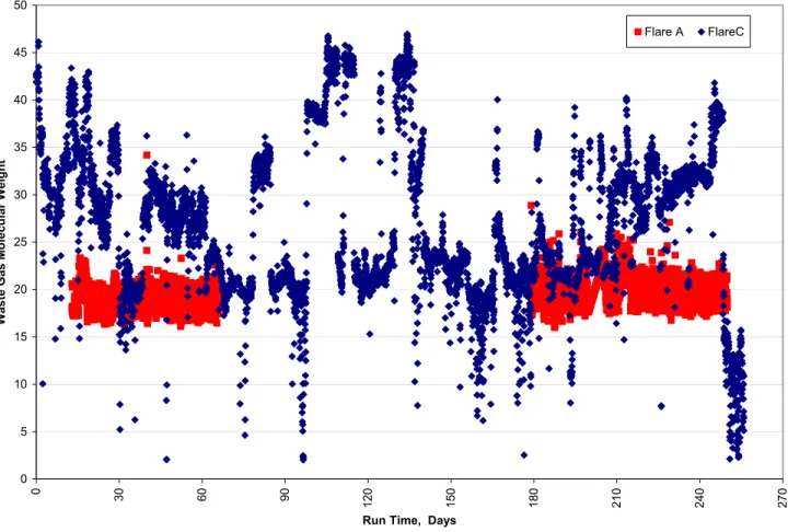
Compositions of waste gases routed to flares can vary significantly depending on the nature of the event(s) that are causing the need to flare waste gas. Sweep or “purge” gas is maintained in the flare header at all times to ensure clear lines and positive flow to the flare tip. Sweep gas normally is natural gas or fuel gas. At low flow rates the sweep gas flow may have a significant impact on the flow and composition measurements depending on the actual locations of the meters and the sweep gas injection point. Figure 4 illustrates the variability in the molecular weight of waste gas observed at two process unit flares, as measured by online flow
Figure 4. Molecular Weight Variations of Waste Gas 0 5 10 15 20 25 30 35 40 45 50 0 30 60 90 120 150 180 210 240 270
Run Time, Days
Waste Gas Molecular Weight
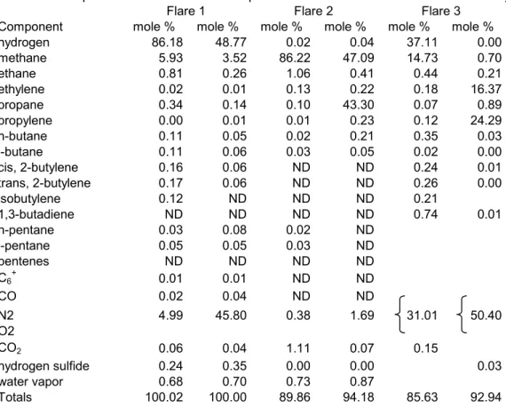
These two examples clearly illustrate significantly different types of flare applications. A flare that is has a relatively consistent composition, and one that sees great changes in composition, in terms of molecular weight and perhaps even in components of interest. Table 1 gives additional examples of waste gas compositions in terms of both constituent of interest and the degree of variation of these components. Table 1 shows 2 cases as measured at different times for each of three flares. Note there is significant variation between the first and 2nd case for each flare. Also note that the recoveries ranged from 89.86 to 100.02 depending on the flare, the components analyzed for, and the components identified. The composition of the waste gas being measured can have a significant impact on the accuracy of many flow measurement technologies. Correcting measured flow rates for these compositional changes will be discussed later.
Table 1. Flare Waste Gas Compositions – Constituents and Variability Table 1. Examples of Flare Waste Gas Compositons-Constituents of Interest and Variability
Component mole % mole % mole % mole % mole % mole %
hydrogen 86.18 48.77 0.02 0.04 37.11 0.00 methane 5.93 3.52 86.22 47.09 14.73 0.70 ethane 0.81 0.26 1.06 0.41 0.44 0.21 ethylene 0.02 0.01 0.13 0.22 0.18 16.37 propane 0.34 0.14 0.10 43.30 0.07 0.89 propylene 0.00 0.01 0.01 0.23 0.12 24.29 n-butane 0.11 0.05 0.02 0.21 0.35 0.03 i-butane 0.11 0.06 0.03 0.05 0.02 0.00 cis, 2-butylene 0.16 0.06 ND ND 0.24 0.01 trans, 2-butylene 0.17 0.06 ND ND 0.26 0.00 isobutylene 0.12 ND ND ND 0.21 1,3-butadiene ND ND ND ND 0.74 0.01 n-pentane 0.03 0.08 0.02 ND i-pentane 0.05 0.05 0.03 ND pentenes ND ND ND ND C6+ 0.01 0.01 ND ND CO 0.02 0.04 ND ND N2 4.99 45.80 0.38 1.69 31.01 50.40 O2 CO2 0.06 0.04 1.11 0.07 0.15 hydrogen sulfide 0.24 0.35 0.00 0.00 0.03 water vapor 0.68 0.70 0.73 0.87 Totals 100.02 100.00 89.86 94.18 85.63 92.94
Flare 1 Flare 2 Flare 3
1.7 Inherent Flow Meter Precision and Accuracy
Each flow measurement device will have an inherent precision and accuracy associated with that technology and model. These metrics will be a function of the fundamental property being measured (e.g. pressure, temperature, frequency, etc.) and the components used in the meter. These metrics are determined under ideal conditions in the laboratory. While the inherent precision and accuracy of the meter is but one of the components that goes into determining the precision and accuracy of the flow measurement in a field application, it is an important
specification to qualify flow measurement technologies. Due to the extreme variations and conditions encountered in flare applications, it is important to have relatively high specifications for the inherent precision and accuracy of flow measurement devices. For this reason an inherent precision specification of +1% and an inherent accuracy of +5% was selected for this study. The reason for selecting such tight inherent flow meter precision and accuracy specifications will be
addressed later in the discussion of the roll up of errors in the overall uncertainty of the mass flow of waste gas to flares.
1.8 Secondary selection criteria
There are a number of other selection criteria, which while important in the selection of a flow measurement device can to some degree be engineered around. These include such
characteristics as applicability to corrosive environments and environments with aerosols and particulate matter. As well as what temperatures and pressures the flow measurement device can be applied. Other factors such as the length of straight pipe required for installation, and the ability to detect backflow in the line can also be of importance. While not primary selection criteria, these characteristics where also assessed for flow measurement technologies which satisfied all of the primary selection criteria.
1.9 Summary
Based upon the above description of flare design and operating parameters the following list of primary design specifications were selected to assess whether available flow measurement technology was applicable to measuring flows in flare systems.
• Applicable in lines from 4”-72” in diameter.
• Maximum pressure drop across measurement device of <0.5 psig.
• Applicable to measurement of velocities from 0-400 ft/sec.
• Quantification of flow (velocities) across 3 decades (1000:1 turndown).
• Inherent flow meter accuracy of + 5 percent.
• Inherent flow meter precision of + 1 percent.
There are a number of secondary criteria such as applicability to corrosive service, specific temperature and pressure constraints, length of straight pipe required, and the ability to sense backflow that are important, but can potentially be engineered around or into a particular
application. These criteria were reviewed and used to evaluate the performance of flow measurement technologies for application in flare service.
2.0 FLARE WASTE GAS FLOW MEASUREMENT
2.1 Flow Measurement FundamentalsVirtually all flow measurement devices calculate volumetric flow by sensing a velocity in the pipe and multiplying that velocity by the cross sectional area of the pipe in which the velocity is being sensed. This velocity is assumed to be uniform across the cross section. Applications where this may not be a good assumption may have reduced precision and accuracy. In fact, the consensus of the flow measurement vendor representatives at a recent API meeting to begin developing an API Standard for measuring flow rates in flares was that the flow profile is the most important consideration in the choice, location, and operation of any flare flow meter.28 Inherent in all of these velocity measurements is an assumption that the gas is of a known composition. Deviation from this assumed composition must be corrected to maintain the overall precision and accuracy of the flow measurement.
2.2 Flow Meter Evaluations
A variety of flow meters were evaluated as a part of this report. The following types of flow meters were evaluated:
Differential Pressure
• Orifice Run with Differential Pressure Taps
• Venturi Run with Differential Pressure Taps
• Pitot Tubes
• Rotameters Mechanical
• Turbines
• Pistons/Disks/Impellers
Mass • Thermal • Coriolis Electronic • Magnetic Meters • Vortex Meters • Ultrasonic Meters
A brief description of the principles of operation for each of these meters and their applicability to flare applications is given in Appendix A. The performance characteristics of each meter type versus the evaluation criteria developed previously for flare systems is summarized in Table 2. If a flow measurement technique failed one or more of the primary evaluation criteria developed for flare systems, it was not considered further. Of the technologies evaluated only constant temperature anemometers (thermal mass meters), pitot tubes, ultrasonic time of flight meters, and possibly a recently developed Doppler shredding vortex meter did not fail one or more of the primary evaluation criteria. However, all of these meters had at least one or more concerns when evaluated against the complete list of flare flow measurement selection criteria. Application of these four techniques to flare applications will be discussed in more detail in the following sections.
Table 2. Flow Meter Selection Table
• See Note At Bottom of Table
Flare Waste Gas Flow Meter Vapor Service Pipe ID Range Backpressure @ Max Design Flow
Obstructs Flare Header Flow Corrosive Service Backflow Measurement Capability Aerosols and Particulates Transmitter Signal Output Straight Pipe Required Principle of Operation Process Velocity Range Process Temperature Range Process Pressure Range Stated Model Accuracy TD Ratio Table I Flow Meter Evaluation Results
Evaluation Criteria Yes 4"-72" <0.5 psig No Yes Yes Yes < 100' 0-1000 FPS -20F to 300F 0 to 60 psig
minimum + 5% 1000:1minimum FLOWMETER Constant Temperature Anemometer (Thermal Mass Meter)
Yes all < 0.1 psig N not
recommended No Yes analog 10 Feet Thermal - Mass0-300 FPS -40C to 200C or 500C model
variation
150 psig 1-3% varying
with TemperatureHigh
Pitot Tubes and
Annubars Yes 0.5 to 72" < 0.5 psig No recommended not Yes Yes (mA) transducer 48 Feet Pressure - Velocity 10 to 1000 FPS up to 546C 2600 psig 1%, depending onapplication
(sensor)
Medium 30:1 Ultrasonic Time Of
Flight Flowmeters Yes 3-120" < 0.1 psig No recommended not Yes Yes 100 Feet time transit 0.1-275 FPS -166 to 300F or 500F optional 1500psig 1 path 3 - 7%, 2 path 2.4 - 5% High 2750:1
Vortex Meters Yes 1-5 or more psig Yes not
recommended
Magnetic Meters No not
recommended
Coriolis Meters Yes < 6" 10 or more psig not
recommended
Dry Test Meters Yes < 6" 1-5 or more psig Yes not
recommended
Wet test Meters Yes < 6" 1-5 or more psig Yes not
recommended
Pistons/Discs/Impell
ers Yes 1-5 or more psig Yes recommended not
Turbines Yes 1-5 or more psig Possibly not
recommended
Rotameters Yes < 4" 1-5 or more psig Yes not
recommended 3-10:1
Venturis Yes 1-5 or more psig Yes not
recommended 3-10:1
Orifice Plates Yes 1-5 or more psig Yes Not
recommended 3-10:1
* Traditional Vortex Meters were ruled out here due to their bluff body design creating excessive pressure drop. A new, novel design, Doppler Shredding Vortex meter that may be able to overcome this limitation was recently developed. According to the Manufacturer and their representative, several of these meters were recently installed in flare headers. The authors have no data or experience with these meters. However, they seem to have potential. Additional information
2.2.1 Pitot Tubes Principle of Operation
A pitot tube calculates a point velocity by measuring the static pressure and the impact or velocity pressure. The static pressure is the operating pressure of the pipe, duct, or stack at a specific point. The impact pressure is a combination of the static pressure and the pressure created by the flowing fluid. Pitot tubes generally measure the impact velocity by situating the opening directly into the oncoming fluid stream. Static ports are often located perpendicular to the fluid flow either on the tube itself or on the pipe or duct. The two pressures create a
differential pressure that is directly related to the velocity through the following equation: Equation 1
(
)
(
)
2
1
/
P
P
C
V
p=
×
T−
S℘
f Where: Vp = Point Velocity C = Dimensional constantρf = Density of the fluid PT = Impact Pressure (a) PS = Static Pressure (b)
This equation gives a linear velocity, not the mass flow rate. The mass flow rate is calculated from the flare header’s cross-sectional area and the molecular weight of the fluid being measured assuming ideal gas behavior of the flared waste gas. In the petrochemical industry, pitot tubes are primarily used to conduct isokinetic sampling traverses in boiler and process heater stacks. The measured flow rate is corrected for the actual fluid using empirically derived K-factors. These measurements are traditionally post-combustion measurements in internal or external combustion device stacks where the gas is primarily air, nitrogen, and water vapor with trace concentrations (<0.1% by volume) of other constituents. Some vendors of averaging pitot tubes are currently advertising them as capable of accurately (within + 2-3%) measuring flows from 10-1000 feet per second in flare headers when used in conjunction with an online gas
Design Variations
There are several variations of pitot tubes: single-port, averaging, area averaging, and s-type. Single-port pitot tubes similar to the one shown in Figure 5, below measure velocity at one point in the flow stream with one static port and one impact port. They are typically used for turbulent streams with well-defined velocity profiles.
Figure 5. Generic Model of Pitot Tube3
To overcome the limitations of a single-port pitot tube, averaging pitot tubes were developed. Averaging pitot tubes have multiple impact pressure and static pressure ports that measure pressure across the pipe diameter. The pressures are tabulated and averaged, thereby negating the issue of placement of a single tube.
Area averaging pitot tubes measure multiple impact and static pressures over the pipe diameter and also over a length of pipe. Area averaging pitot tubes usually are comprised of several sets of pitot tubes connected to a manifold. These are typically used for large stacks or ducts. S-type pitot tubes are specially designed to withstand dirty flows with a high level of particulate matter. Any of the above instruments could employ the s-type design for use in flows with high levels of particulate matter. For flare applications averaging pitot tubes are typically used. For the remainder of this section the applicability of pitot tubes to measuring flare flows will be discussed.
Applicability to Flares
Pitot tubes have been used for years to measure flare flows. This is primarily because until fairly recently pitot tubes were the only viable flow measurement option. Although pitot tubes are fully capable of measuring flare flows, they may not be the best solution for all applications. Using an averaging pitot tube to measure flare flow has several positives; but there are several limitations to the design and operation of the device as compared to some newer waste gas flow measurement technologies.
Pitot tubes are capable of meeting the data quality objectives of this study across a limited range of flows (10-1000 feet/second). However, the stipulation that the flow meters measure through the entire range of the potential flow may cause problems for pitot tubes. As stated previously, flares are capable of having wide ranging flare flows, upwards of 100-1000:1. A typical
averaging pitot tube turndown ratio is 30:12. A particular problem with pitot tubes is their ability to measure low flows in large diameter pipes, as the pressure differentials that must be sensed are quite low. To accurately measure over the entire possible design window for flares would
require multiple pitot tubes calibrated over several ranges of flow. While this could be considered an acceptable approach to measuring flare waste gas flow rates, this has to the authors’ knowledge not been done. Several flow meter suppliers are now offering multiple ranges averaging pitots, but there is limited data available on their use in flare applications. Under ideal conditions the precision and accuracy of pitot tubes is quite good. For example, the quoted accuracy of the Dieterich Standard Diamond II Annubar is +1% with a precision of 0.1% for the sensor3. Ideal conditions for pitot tubes are stable flows, operating temperatures and pressures, and constant density of the stream being measured. These unfortunately are not common conditions in most flare applications. Correcting for the actual gas composition in most cases will induce as much or more uncertainty into the flow measurement than the inherent error of the flow meter being used. A more detailed discussion of the roll-up of error in flow
measurements is presented in Section 4.0, but in most field applications of pitot tubes in waste gas service the total uncertainty of the flow measurement will be in the range of 5-20 percent. The exact value being a function not only of the inherent uncertainty of the flow meter, but also of the variability of the gas composition and one’s ability to measure and compensate for the actual gas composition.
Pitot tubes require a rather large amount of straight run piping prior to the device. If
straightening vanes are not used, a straight run of between 10-25 pipe diameters is often quoted. Typical downstream straight pipe run requirements are 5-10 diameters. In many flare
applications this may not be an issue due to the length and amount of piping needed to transport the flare gas to the remote areas usually used for flare locations. Where space is limited and the flare stacks are very near the flare knockout drum, this 10-25-pipe diameter requirement will definitely be problematic. Straightening vanes or other flow correcting devices can be used to minimize the impact on observed meter accuracy of not having the desired runs of straight pipe for installing pitot tubes. However, the installation of straightening vanes and/or other flow correcting devices in flare headers can pose a serious safety hazard, due to the potential to collect debris and inhibit flow, and may not be allowed in many flare installations.
Other than applications requiring straightening vanes, the application of pitot tubes to flare systems should not pose any significant safety risk. The actual instrument is a slim, aerodynamic tube that does not obstruct the flow enough to be of significant concern for collecting
hydrocarbons. Additionally there are no mechanical or moving parts that could be affected by electrical problems. Pitot tubes also induce very low-pressure loss across the device due to the unobtrusive design, typically less than 0.5 psig. One potential problem area for pitot tubes is measuring flows in corrosive service or applications with high levels of particulate matter. The pressure ports are prone to plug when used in dirty flows. Some designs attempt to alleviate this problem by using larger size portholes or flushing the holes with an inert gas. Periodically cleaning the ports and checking the differential pressure cell ensures device accuracy and usually is a routine task. Annual calibrations may also be required to ensure accurate performance. Pitot tubes can be used to measure flows in virtually any size pipe. Pitot tubes can be installed in piping in excess of 48" without incurring additional costs for installation. For example, the Diamond II+ Annubar is capable of being installed in piping from 0.5” to 72". 3 Additionally, most pitot tubes can function across a wide range of temperatures and pressures, up to 546oC and 2600 psi. This is well within the operating range for almost all flares in terms of temperature and pressure.
In the authors’ experience, pitot tubes were originally installed in many flare headers to measure waste gas flow rates for informational purposes rather than for critical process controls or meeting regulatory requirements. Typically, the pitot tubes ports were found to have “plugged
up” from salts, polysulfides, ammonium sulfide, and other particulates that may form in flare headers from time to time. Also, many of the originally installed pitot tubes were found to be bent or broken as a result of maintenance activities on the flare headers. Typically, since the flow signal was not a critical control variable or a compliance parameter, the level of
maintenance was not adequate to keep the pitot tube functioning. Also, the readings from these meters became more and more suspect as additional sources were tied into the flare line thereby increasing the potential for the waste gas composition to vary considerably.
2.2.2 Thermal Mass Meters Principle of Operation
Thermal mass flow meters operate on the principle of measuring temperature differences between two sensors. Generally, a unit contains two temperature sensors, such as
thermocouples, and a heating element. The temperature difference between the two sensors is a function of the flow past the sensor. There are two methods to achieve the temperature
differential, constant temperature and constant power.
In the constant power approach, one of the sensors receives a constant supply of energy, or heat, from an electric heater. The temperature rise of the sensor is measured as well as the heat supplied. The other sensor measures the operating temperature of the fluid.
The constant temperature approach maintains one of the sensors at a specific temperature above operating conditions. The amount of energy needed to maintain the temperature is measured and used to compute a mass flow rate. As in the previous method the second sensor measures
operating temperature conditions.
One recently developed constant temperature thermal mass meter has two sets of sensors with one set in the traditional waste gas flow area and the other set very near the flare header wall. According to the vendor, this allows the meter to continually measure both a waste gas flow and a near-zero flow in real time. 29 Having two pairs of sensors, one in the main waste gas flow stream and one near the walls, allows the meter to obtain a flowing stream waste gas velocity and a near zero waste gas velocity. One pair of sensors could conceivably give the same velocity reading for two or more widely varying gas mixtures. According to the vendor29, no two gas compositions will have identical velocity readings at both the in stream velocity and at a near
zero velocity. Thus, the meter is able to identify the actual composition of the waste gas by comparing the two readings and correct the velocity measurement for the actual composition in real time.
The underlying equation governing both methods of thermal mass flow meters is essentially the same: Equation 2:
(
)
[
C
pT
2T
1]
KQ/
M
=
−
Where:M = Mass flow rate K = Meter coefficient
Q = amount of energy supplied Cp = specific heat of the flow
T2 = Temperature of the constant power sensor T1 = Temperature at operating conditions.
Per Equation 2, one can see that the observed flow from a thermal mass meter requires
knowledge of the gas composition. Any significant deviation in composition of the waste gas being measured from the composition of the gas on which the meter was calibrated will impact the accuracy of the observed flow measurement. While real time correction of thermal mass meters for changes in gas composition are possible (correction for variable gas composition will be discussed further in Compositional impacts on calibration), there are a limited number of applications where this has been done in the petrochemical industry.
Design Variations
There are several variations of thermal mass flow meters that use one of the methods mentioned above to measure mass flow rate including heated tube designs, bypass, insertion probes, and hot wire anemometers. Heated tube mass meters are designed to protect the heater and temperature sensor elements from corrosive or dirty flows. The heater is mounted on the outside of the pipe and directly heats a section of the pipe wall. One temperature sensor is situated far enough downstream of the heater to measure operating temperature conditions. A second sensor is upstream in close proximity with the electric-driven heater. The mass flow rate is a nonlinear
function of the heat transfer of the pipe walls and the sensor. Bypass thermal mass meters are generally used in high flow, high-pressure applications. Essentially a portion of the flow is bypassed into a tube that is heated. A portion of the energy is transferred to the gas, which is measured by temperature sensors. Due to the bypassing of flow, a large pressure drop is incurred across this type of meter, and generally is not suitable for flare applications.
Figure 6. Generic Example of Thermal Mass Flow Meter 4
Insertion probes use the constant temperature method stated above except the sensors or probes are inserted into the flow stream. One sensor is maintained at a constant temperature above ambient conditions. The energy necessary to maintain the temperature is recorded and used to calculate mass flow. Hot wire anemometers use the same principles as constant-temperature or constant-power mass flow meters. Anemometers use thin filaments to measure the heat transfer between a reference and a heated sensor.
Thermal mass meters are capable of obtaining and relaying continuous measurements. There are several current petrochemical industry examples of this process. Turndown ratios are a minor issue for thermal meters as most can quantify flow velocities across a two-decade range (100:1) or more. Flares can have turndown ratios of 1000:1; therefore the use of two or more thermal meters may be necessary to cover the whole range of flow seen in these applications.
The quoted accuracy from the K-bar 2000 from Kurz Instruments is listed as +1-3%, depending on operating temperature.69 Because thermal mass meters require the composition of the gas to be known to compute the flow, the uncertainty of the flow will also be a function of the
uncertainty of the gas composition. In the authors’ experience, total flow measurement error can be in the 5-10% range and could be as high as 20% in applications with widely varying
compositions. Correcting measured linear velocities to actual mass flow rates can be problematic if the molecular weight of the waste gas varies by more than 20% from the molecular weight of the meter’s calibration gas. [More detail on this problem is presented Section 2.3 “Factors Influencing Measurement Performance”.] The repeatability of the instrument is given as 0.25%4.
Many source-testing protocols dictate that flow meters have a minimum of 8 pipe diameters of straight pipe upstream and 2 pipe diameters of straight pipe downstream of the meter to ensure consistent velocity and velocity profiles. For most circumstances, thermal meters do not require additional space beyond these requirements. It is possible to install thermal meters by inserting them through existing gate valves on flare lines or permanently installing by hot-tapping into the flare system. Thermal meters do not present safety concerns as they induce very little pressure drop and do no not act as an obstruction in most circumstances. The instrument has low-pressure drops (< 0.1 psig) due to the unobtrusive design. Typical thermal meters consist of a metal probe that houses two thermal transducers. Corrosive or hazardous flows may be a problem for carbon steel instruments, but most instruments are typically constructed of stainless steel or other materials that resist corrosion or rusting.
Thermal meters can be used across a wide range of temperatures and pressures, and for the most part are unaffected by density, viscosity, pressure, or temperature fluctuations. Therefore, process conditions tend to not be an issue when evaluating the applicability of a thermal mass meter. For example, the operating limits for the K-bar 2000 can range from -40 to 500oC over a pressure range of 150 psig. The flow meter is designed to measure flows from 0-18000 standard cubic feet per minute (SCFM).
Thermal meters can be installed in pipe sizes well in excess of 48 inches. Typical costs of thermal meters are between $3,000-$5,000. Permanent installment increases the cost as does harsh operating conditions and maintenance due to operator error. Flows with high levels of particulate matter may induce error by coating the transducers and limiting transducer life. Typical maintenance for thermal flow meters consists of periodic cleaning of the transducers. In severe applications additional particulate removal equipment or frequent meter change outs may
4http://kurzinstruments.com/K-BAR1.pdf
be required to keep the meter functional. When thermal mass meters are removed from the flare header for cleaning or being moved to new locations (temporary installations) care must be taken when removing and reinserting to avoid damaging the transducers. Additionally, annual
calibrations of the probe may be required in order to ensure accurate measurement.
One drawback of thermal meters is the inability to measure bi-directional flow and compensate for backflow. Unlike most other flow meters, thermal mass meters are not unidirectional,
meaning that they sense flow in either direction as a positive signal. While this would be of little concern when detecting flows at the terminal end of a flare system, it may be a confounding factor when using a thermal mass meter to detect the source of waste gas flows in a complex flare piping system.
Applicability to Flares
Both constant-power and constant-temperature thermal meters have been used to measure petrochemical industry waste gas flows to flares. John Zink engineers use thermal mass meters exclusively in measuring flare header waste gas flows for designing flare gas recovery
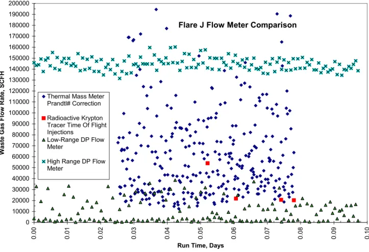
compressors. Several petrochemical facilities use thermal mass meters to isolate potential sources of flows to flare headers. One petrochemical facility has over 50 thermal mass meters installed for this purpose. The authors’ experience is that thermal mass meters are more reliable than pitots since they aren’t as prone to the mechanical integrity problems mentioned previously concerning pitot tubes. Figure 7 shows a comparison of flare waste gas measurements between single point pitot tubes and thermal mass meters. Note that both the high-range and low-range pitot tubes only provide measurements over a narrow range at each end of the measured flows while the thermal mass meter covers the entire range. Also, note that the flows in Figure 7 are in typical flare waste gas ranges all of which both the thermal mass meter and the pitot tube
vendors claim they can handle accurately. Using the pitot tubes only, one could conclude that either the low or high flow pitot is not giving accurate readings and base the measurements on either a very high or a very low flow compared to the oscillating flow rates as measured by the thermal mass meter and the tracer injections. This can be particularly misleading for flare systems that are subject to surge or oscillating flows, as was the case for this example.
Flare J Flow Meter Comparison 0 10000 20000 30000 40000 50000 60000 70000 80000 90000 100000 110000 120000 130000 140000 150000 160000 170000 180000 190000 200000 0.00 0.01 0.02 0.03 0.04 0.05 0.06 0.07 0.08 0.09 0.10
Run Time, Days
Waste Gas Flow Rate, SCFH
Thermal Mass Meter Prandtl# Correction Radioactive Krypton Tracer Time Of Flight Injections
Low-Range DP Flow Meter
High Range DP Flow Meter
Figure 7. Comparison of Various Flow Measurement Techniques
2.2.3 Ultrasonic Time-of-Flight Meters Principle of Operation
There are two types of ultrasonic flow meters, Doppler shift and transit time. Flow meters that use Doppler shift technology rely on the principle that wavelengths are perceived as shorter as the source approaches and longer as the source retreats. In fluid applications, Doppler shift flow meters are anchored or clamped onto the pipe and house a transmitter and a receiver. The transmitter emits signals that are reflected back to the receiver by discontinuities in the flowing fluid such as air bubbles, particles, or other turbulent phenomena. The receiver detects the change in wavelength of the signal reflected from these discontinuities in the flowing fluid, rather than the fluid itself. For this reason Doppler shift only works on fluids with appreciable levels of discontinuities. The underlying equation governing flow meters using Doppler shift is:
Equation 3:
(
f
f
)
K
V
=
o−
1Where:
V = Velocity of the fluid fo = transmitter frequency f1 = receiver frequency
K = constant of the transmitter and system
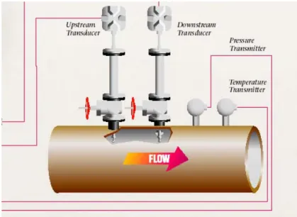
Figure 8. Generic Example of Ultrasonic Flow Meter5
5http://www.gepower.com/dhtml/panametrics/en_us/products/ultrasonic_gas_flow meters/gf868_flare_gas_flow meter.jsp
Flow meters that operate on transit time measurement operate on the principle that ultrasonic signals travel faster with the flowing fluid and slower when traveling against the flowing fluid. Typically, one transducer is mounted upstream while another is mounted downstream at a fixed separation. The transducers act as transmitters and receivers alternatively, and emit and receive sound waves simultaneously. Waves that travel with the fluid flow exhibit a faster velocity than waves that travel against the flow, giving a differential time. In the absence of flow, sound waves travel from both transducers to each other in the same amount of time, therefore the differential is zero. The basic equation used to calculate the velocity of the fluid is37: Equation 4:
⋅
−
=
12 21 12 21 22
T
T
T
T
X
L
V
1 Where:V = Velocity of the flow
L = direct distance between transducers X = lateral distance between transducers
T21 = travel time from downstream transducer to upstream transducer T12 = travel time from upstream transducer to downstream transducer
An additional advantage of ultrasonic time of flight meters is that the differential times may also be use to solve for the speed of sound in the flowing gas. For an ideal gas the speed of sound, c, can be related to the molecular weight of the gas by the following,39
Equation 5:
MW
RT
c
=
γ
/
Where:
c = speed of sound in gas R =universal gas constant T = absolute temperature γ = specific heat ratio
Thus, in addition to the velocity of the gas, ultrasonic time of flight meters can be used to
estimate the molecular weight of the gas. This allows one to estimate the mass flow rate without doing any other composition measurements.
Design Variations
Aside from the design variations involved with Doppler shift and transit time, ultrasonic flow meters come in portable clamp-on models and installed tap-in models. While clamp-on Doppler shift meters have been used successfully to measure liquid flows, where substantial flow
disturbances or particulate matter may be present, the authors are aware of no clamp-on Doppler shift meters used in gas service. The current generation of portable, clamp-on, transit time flow meter requires pressures approaching 80 psig or more when measuring gaseous flow. Thus, portable clamp-on transit time meters are not applicable to measuring waste gas flows in near atmospheric pressure flare headers. For petrochemical industry flare applications, permanently installed transit time devices are used. Available literature indicates that well over 2000 time of flight ultrasonic flow meters have been install in flare applications worldwide.76 The remainder of this section will focus primarily on permanently installed transit time models.
Transit time flow meters are capable of providing continuous flow measurements and there are many industry applications. Ultrasonic flow meters are capable of handling very large ranges of flows, as is prevalent in flare systems. One supplier gives a typical turndown ratio of 2750:1, over a flow range of 0.1 to 275 ft/s.5 As with most flow meters, the accuracy declines at very low and very high flow rates. For ultrasonic time-of-flight meters, the high level of sound at high flow rates (above 275 feet per second) makes it impossible to obtain a reading forcing their inaccuracy to approach infinity. At very low flow rates (<0.1 feet per second); the very low level of sound makes the sound very difficult to detect.
Panametrics quotes the accuracy of the Digital Flow GF868 Mass Flow meter at + 2-5% at a velocity range of 0.1-275 ft/s and measuring gas of the same composition as that used to calibrate the meter.5 However, actual accuracies depend on transducer design, electronics installed, flow rate, the actual composition of the waste gas, and the profile of the actual flow. Accuracies may range from 5-10% or higher with additional error incorporated for additional pieces of equipment and operating conditions (see Section C Factors influencing measurement performance). The quoted precision for the instrument is given as 1 percent.5 Transit time
models are claimed by the vendors to be the most accurate of all the flow meters currently used to measure flare or waste gas flows.
Manufacturers of transit time meters suggest installing the meter in a straight run of pipe with upstream to down stream ratios of straight pipe of 20 pipe diameters upstream and 10 pipe diameters downstream to ensure a smooth velocity profile and accurate performance. This may be an issue in flares that do not contain the necessary piping. As mentioned for pitot tubes, straighten vanes or other flow correction devices may be used in some applications to correct for not having enough straight pipe run, but due to safety concerns they may not be utilized in many applications.
Ultrasonic flow meters do not obstruct the flare lines and are not indirect safety hazards. Most meters consist of transducers that are slim in design and do not inhibit the flow of material. Due to the unobtrusive design, ultrasonic flow meters also offer negligible pressure drop (<0.1 psig) across the device. This, as stated in previous sections, is an important consideration due to the low operating pressures of most flares. Ultrasonic time-of-flight meters can also handle
corrosive or hazardous flows with additional material expense incurred. Typically, all the parts of the meter exposed to the waste gas are made of stainless steel or other specialty materials making them appropriate for most petrochemical industry applications. For very harsh
applications, it is possible to design the parts of the meter that come in contact with the waste gas using more expensive specialty materials.
Ultrasonic transit time meters are available for application in piping from approximately 3” up to 120",5 which make them applicable to the large pipe sizes frequently found in flare systems. These meters may be used across temperature ranges of -110 to 150° C and pressures up to 1500 psig. Ultrasonic meters can accurately measure bi-directional flow due to the design of the meter. One transducer acts as an accelerated sound wave, while the second acts as a retarded wave. In the event of bi-directional flow the transducers simply measure this as a negative flow. The instrument can calculate the actual positive flow by adding the negative number from one transducer to the positive number from the other transducer. Additionally, ultrasonic meters can operate in flows that have a fairly high level of particulate matter. Past designs often had
induced error associated with flows with high levels of particulate matter, however current models have been specifically designed to overcome these limitations. Changes to the design to reduce waste gas particulate limitations include orienting the two transducers at a 45 degree
angle, decreasing the diameter of the transducer probes, and reducing the distance the transducer probes intrude into the flare header line. Additionally, process changes driven by regulatory requirements and economics reduced the particulate levels in flare waste gas considerably from those originally encountered.
Ultrasonic meters are typically permanently installed into the flare line and require a unit shutdown for installation. Some models can be hot-tapped into the process and are portable. However, some petrochemical facilities do not allow hot tapping of flare lines under any circumstances while many others only allow hot tapping under very specific process conditions due to safety concerns around the flare. In these cases, it may be necessary to take the flare out of service to install the meters.
For the most part ultrasonic transit time meters require little maintenance in order to ensure accurate performance well within the stated TCEQ data quality objectives. Panametrics states in the brochure for the GF868 mass flow meter that the unit "does not require regular maintenance", "has no moving parts to clog or wear", and " is constructed of titanium or other metals that withstand the corrosive environment usually found in flare gas applications". 5 Annual calibrations of the meter may be necessary to ensure accurate performance.
Applicability to Flares
Ultrasonic transit time meters have successfully measured flare flows in refineries and in flare gas applications. Since ultrasonic time of flight meters do not have to be corrected for varying gas composition, and in fact can be used to estimate the molecular weight from the observed speed of sound, they are in many instances the preferred flow meter for flare applications. One drawback to the time transit flow meter is the high purchase and installation cost. Typical costs for an ultrasonic time-of-flight meter are in the $20,000-30,000 range. The author’s experience is that design, site preparation, installation, field calibration, and connecting the meter to the distributed control system typically make the overall up-front cost for an ultrasonic time-of-flight meter approach $100,000.
2.2.4 Combination Systems
Because of the potential large dynamic range of velocities that can be encountered in flare systems, there has been some interest in flow measurement systems that use a combination of
flow measurement technologies to cover different ranges of the flow spectrum (multiple range averaging pitots, time of flight meters used in conjunction with high flow pitots, etc.). While there are several vendors whose product literature mentions such combination systems, the authors were not able to identify any such systems that had been installed in flare systems to date. In theory extending the range of velocities that can be measured should be possible by combining flow measurement technologies to cover different ranges. The relative strength and weaknesses of the individual technologies is largely unchanged by combining them into an integrated flow measurement system. However, there are some inherent problems with matching the flows measured in the region where their measurement capability overlap and it remains to be demonstrated in a full scale application. In most cases the advantage of such a combined system may be to extend the range to cover large design case release scenarios that may seldom or never be seen. It is unclear to the authors whether this seldom-used extended range will warrant the additional complication of a combined flow measurement system.
2.3 Factors Influencing Measurement Performance 2.3.1 Measurement Uncertainties
The types of flow meters acceptable for flare measurement service have some differences in the standard accuracy and precision responses. The data for these metrics are shown in Table 2, along with other comparative data that will be discussed later.
One vendor of ultrasonic flare gas meters quotes velocity measurement accuracy within + 1.4 to + 3.5% 5. However, using the vendor-supplied parameters in the International Organization for Standardization (ISO) TR 5168 root sum square model 6 results in a higher measurement error. This model, given in Equation 6, can be used to estimate flow measurement inaccuracy with a 95% confidence interval based on the principal sources of uncertainty in the measurement,
Equation 6
Overall Error =
(Vo)2
+
(So)2
+
(To)2
+
(Po)2
+
(Do)2
Where:
Vo = Gas velocity uncertainty (Per vendor + 1.4 to 3.5 % for a 2 path flow meter and velocities between 1 and 275 feet/second)
So = Uncertainty in speed of sound for gas being measured (+ 1.0% per vendor) To = Gas temperature uncertainty (+ 2% per Rule 115 requirements)
Po = Gas pressure uncertainty (+ 5mm Hg per Rule 115 requirements is ~0.66%)
Do = Pipe inside diameter uncertainty (+ 0.5% per Shell Flow Meter Engineering Handbook 14) Insertion of the above values into the equation results in an overall uncertainty of + 2.75% to + 4.25% for ultrasonic flow meters, depending on the gas velocity uncertainty.
For thermal mass meters, vendors quote 0.25% repeatability, + 0.5% of temperature reading for velocities above 100 standard feet per minute (SFPM, velocity of air at standard temperature and pressure conditions) and with optional velocity/temperature/mapping an overall accuracy of + [3% of the reading +(20 SFPM +0.25 SFPM/°C], above or below 25°C. Using the same values above for errors in temperature, pressure, and diameter together with the minimum + 3%
accuracy quoted for thermal mass meters, and neglecting the speed of sound term (does not enter in the uncertainty of thermal mass meters), results in a minimum overall error of + 3.8% for thermal mass meters.
As mentioned earlier one vendor of pitot tubes claims overall accuracy of + 1%. Using the same values above for errors in temperature, pressure, and diameter together with the quoted + 1% accuracy and neglecting the speed of sound term (does not enter into the uncertainty of pitot tubes) results in a minimum overall error of + 2.6%.
These uncertainties only represent the inherent uncertainty of the input variables measured to derive the flow measurement. For all the meters there is also an uncertainty associated with the composition of the gas being measured. For ultrasonic meters the uncertainty of the gas
composition can be estimated directly from the input variables measured by the flow meter by using equation 6 and the speed of sound derived from the flow meter. However, for pitot tub