Technological University Dublin Technological University Dublin
ARROW@TU Dublin
ARROW@TU Dublin
Dissertations School of Computing
2017
Critical Comparison of the Classification Ability of Deep
Critical Comparison of the Classification Ability of Deep
Convolutional Neural Network Frameworks with Support Vector
Convolutional Neural Network Frameworks with Support Vector
Machine Techniques in the Image Classification Process
Machine Techniques in the Image Classification Process
Robert KellyTechnological University Dublin
Follow this and additional works at: https://arrow.tudublin.ie/scschcomdis Part of the Computer Engineering Commons
Recommended Citation Recommended Citation
Kelly, R. (2017) . Critical Comparison of the Classification Ability of Deep Convolutional Neural Network Frameworks with Support Vector Machine Techniques in the Image Classification Process. Masters dissertation, Technological University Dublin, 2017. doi:10.21427/D7SS4S
This Dissertation is brought to you for free and open access by the School of Computing at ARROW@TU Dublin. It has been accepted for inclusion in Dissertations by an authorized administrator of ARROW@TU Dublin. For more information, please contact
[email protected], [email protected], [email protected].
This work is licensed under a Creative Commons Attribution-Noncommercial-Share Alike 3.0 License
Critical Comparison of the Classification Ability of Deep
Convolutional Neural Network Frameworks with Support
Vector Machine Techniques in the Image Classification
Process
Robert T. Kelly D14126766
A dissertation submitted in partial fulfilment of the requirements of Dublin Institute of Technology for the degree of
M.Sc. in Computing (Data Analytics) 25/01/2017
ii
Declaration
I certify that this dissertation which I now submit for examination for the award of MSc in Computing (Data Analytics), is entirely my own work and has not been taken from the work of others save and to the extent that such work has been cited and acknowledged within the test of my work.
This dissertation was prepared according to the regulations for postgraduate study of the Dublin Institute of Technology and has not been submitted in whole or part for an award in any other Institute or University.
The work reported on in this dissertation conforms to the principles and requirements of the Institute’s guidelines for ethics in research.
Student Name: Robert Kelly
Signed: ………
iii
Abstract
Recently, a number of new image classification models have been developed to diversify the number of options available to prospective machine learning classifiers, such as Deep Learning. This is particularly important in the field of medical image classification as a misdiagnosis could have a severe impact on the patient. However, an assessment on the level to which a deep learning based Convolutional Neural Network can outperform a Support Vector Machine has not been discussed.
In this project, the use of CNN and SVM classifiers is used on a dataset of approx. 55,000 images. This dataset was used to assess the classification potential of each methodology, in terms of training, implementation, and the ability to engineer parameters and features for successful classifications on a very large dataset. The use of CNN approaches is further broken down into the use of different frameworks, in this case Theano and Torch implementations. These are then compared to an SVM classifier by confusion matrix, training time and ease of use to assess which has the higher classification potential.
Here it is seen that the Theano model outperforms the Torch model slightly for this task, by roughly 3% in the accuracy of the confusion matrix. The SVM meanwhile is shown to be very limited in its ability to classify such a large dataset. Furthermore, the SVM is shown to be limited in its ability to recognise the classes corresponding to the different levels of disease severity, achieving a classification accuracy of only 75% for the whole sample.
These results suggest that the application of Deep Learning techniques currently have a very large advantage over SVM approaches in both accuracy and data handling, that to not natively avail of the computational power of Deep Learning.
Key Words: Deep Leaning, Neural Networks, Support Vector Machines, Medical Image Classification, Theano, Torch
iv
Acknowledgements
This was a very long work in progress and it is thanks to the perseverance and understanding of a number of people that it has been eventually completed
First, to John McAuley for enormous support and encouragement throughout the process, without whom I would have been unlikely to finish this work, and who was given the unenviable task of keeping this on track at times when it was completely up in the air.
Second, I would like to thank the staff of the DIT School of Computer Science, particularly Luca Longo, Sarah Jane Delaney and Andrea Curley for boundless support and understanding at a very busy time in my life.
Third, to my colleagues at Deutsche Bank, who were very supportive to the completion of this work at the expense of having to pick up the slack I left on the team while completing this.
Finally, to my family, my partner Shane-Liz Andaloc and my daughter Jasmine Andaloc-Kelly. Having a baby during the completion of this project, was both one of the most stressful and the most rewarding experience of my life. This work would not have been possible without the unbelievable patience and understanding of my partner, and I am endlessly grateful for this, and am finally able to take up my share of the baby changing responsibilities.
v
Table of Contents
Declaration ... ii
Abstract...iii
Acknowledgements ... iv
Table of Figures ... vii
Table of Tables ... viii
1. Introduction ... 9
1.1. Background ... 9
1.2. Research Question ... 10
1.3. Hypothesis and Research Objectives... 10
1.4. Research Methodologies ... 11
1.5. Thesis outline ... 11
2. Literature Review and related work ... 13
2.1 Diabetic Retinopathy Background ... 13
2.2. Machine Learning Classifiers... 14
2.3. Support Vector Machines ... 15
2.4. Convolutional Neural Networks ... 18
2.4.1. Convolutional Layers ... 18
2.4.2. Pooling Layers ... 19
2.4.3. Fully Connected Layers ... 20
2.5. Model Performance Measurements ... 20
2.6. Deep learning and GPU computing ... 23
2.7. Summary ... 24
3. Design and Implementation ... 25
3.1. Data ... 25
3.2. SVM Configuration ... 26
3.3. CNN Configuration ... 26
3.4. Summary ... 27
4. Implementation and Results ... 28
4.1. Image Pre-Processing ... 28
4.2. Development of SVM ... 31
4.3. Development of CNN ... 33
4.3.1. Theano Implementation... 33
vi
4.4. SVM Implementation ... 39
4.4.1. Grey Scale Conversion ... 39
4.4.2 Adaptive Histogram Equalisation (AHE) ... 40
4.4.3. Wavelet Transformation ... 41
4.4.4. Principal Component Analysis ... 41
4.4.5. Fuzzy c-Means Clustering ... 42
4.4.6. Feature Extraction ... 42
4.4.7. SVM Classification ... 42
4.5. Summary ... 43
5. Evaluation and Analysis ... 45
5.1. CNN Evaluation ... 45
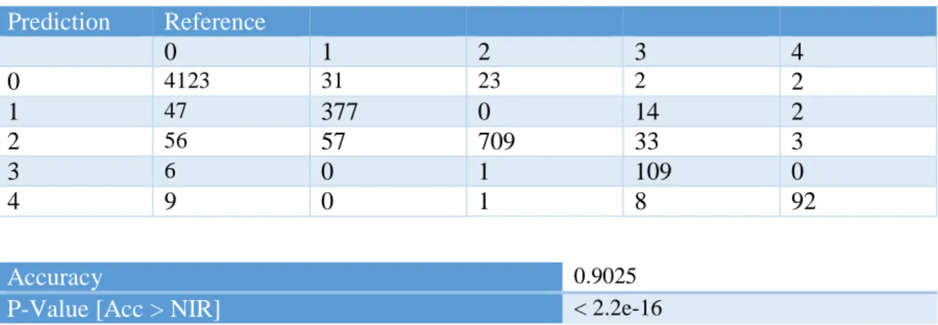
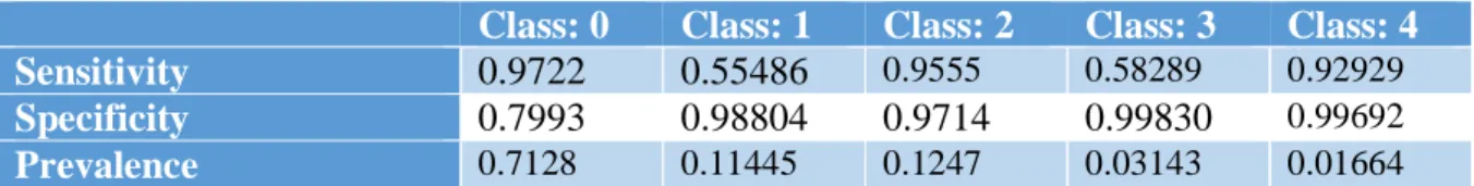
5.1.1. Model Accuracy Measures ... 48
5.1.2. CNN Model Selection ... 51 5.2. SVM Evaluation... 51 5.3. Summary ... 54 6. Conclusion ... 55 6.1. Research Objectives ... 55 6.2. Future Work ... 57 Bibliography ... 60
Appendix 1: Confusion Matrixes and Classification Results ... 64
Theano CNN Complete Confusion Matrix and Descriptive Statistics ... 64
CNN classification results ... 65
SVM Complete Confusion Matrix and Descriptive Statistics ... 66
SVM Classification Results ... 67
Appendix 2: Python Model Codes ... 68
Image Conversion Code ... 68
Theano (lasagne) Neural Net Training Script... 71
Theano Transform File ... 72
Theano Blend Script (Part) ... 74
SVM Model Generation Code ... 76
Supplementary codes ... 78
vii
Table of Figures
Figure 1:Project workflow diagram ... 12
Figure 2: Support Vector Machine Overview ... 17
Figure 3: Convolutional Neural Network Overview ... 20
Figure 4: Machine learning performance measurement ... 22
Figure 5: Source training images ... 29
Figure 6: Border Removal ... 29
Figure 7: Collage of Transformed images ... 30
Figure 8: Theano Network architecture... 34
Figure 9: Torch network architecture ... 37
Figure 10: Montage of pre-processed images and the resulting greyscale images ... 40
Figure 11: Results of the AHE pre-processing stage ... 40
Figure 12: Results of the wavelet transformation step of the feature engineering stage ... 41
viii
Table of Tables
Table 1: Theano Blend Network Architecture ... 36
Table 2: Summary of the various models being investigated and the parameter and feature engineering tasks involved with their development. ... 44
Table 3: Theano CNN Confusion Matrix ... 48
Table 4: Torch CNN Confusion Matrix ... 49
9
1. Introduction
In this section, the background scope for the study will be introduced, the research question will be presented, the hypothesis and research objectives will be stated and the data source will be specified. Finally, an overview of this thesis and its contents will be presented.
1.1. Background
Many people consider dynamic parallelism to be the future of computing as future microprocessor development will likely focus on the addition of cores to the processor system. However, it is difficult to fully integrate all CPU cores as a fully parallel system. The architecture of a graphics processing unit (GPU) allows for parallelisation as these features are necessary to render and perform computationally difficult visualisations (Merrill & Grimshaw, 2011; Owens et al., 2008).
Since its induction, a number of applications have benefited greatly from the application of Deep Learning within the field of data analytics. One such example is the field of medical imaging, which was one of the first “early adopters” of GPU programming. As patient numbers, and hospital waiting times, continue to increase, automating the diagnostic process could free up time for medical researchers to deal with more patients in the same period of time. This would also allow patients to receive a diagnosis at an expedited pace.
While a number of papers have sought to understand the performance gains possible through Deep Learning and GPU computing, information on the time saved carrying out classification of large medical image datasets is scant (Pratx & Xing, 2011; Schmidhuber, 2015)
This study intends to investigate the classification of images using modern Deep Learning based approaches and quantitatively assess to what extent they can outperform more traditional CPU based techniques. While previous works (Bandyopadhyay & Sahni, 2011; Cheng & Wang, 2011; Schmidhuber, 2015; Tarditi, Puri, & Oglesby, 2006) have identified a correlation between the addition of GPU technology to an algorithm, and an increase in performance, it has not been completely assessed to what level there will be an increase in image classification using high resolution images.
Image classification is a well-known quantity, and it is possible to use a number of techniques to implement it. The addition of Deep Learning techniques allows for the implementation of Convoluted Neural Networks (CNN), which have been shown to allow for
10
increased speed and fidelity in classification procedures in other studies. In contrast to other machine learning techniques, CNN’s do not require an overly large training time, therefore the model production can be expedited. To compare and contrast the performance increases, traditional neural networks and support vector machines will be used for comparison, as they have also been shown to have strong abilities to classify images.
1.2. Research Question
The research question that this study seeks to address is: To what extent can deep learning based neural networks statistically out-perform Support Vector Machines for image classification and under what circumstances could other Support Vector Machines be considered more useful?
1.3. Hypothesis and Research Objectives
H0: This is the null hypothesis. The application of Deep Learning will result in no performance increase over CPU approaches and will result in similar training times.
H1: The addition of Deep Learning and GPU computing techniques by way of Deep Convoluted Neural Networks will allow for a decrease in misclassification rate over a traditional neural network classification or Support Vector Machine (SVM).
H2: Training time will be greatly reduced when using Deep Learning compared to a traditional CPU based approach
This project will involve carrying out secondary research, using quantitative approaches, to empirically classify a best practice method of image classification using deductive reasoning. Data will be generated using the suggested datasets, split between a training a test set. Using these datasets, a comparative study between deep learning and traditional image classification tests will be carried out.
11
1.4. Research Methodologies
The data for this study is a large medical image dataset, focusing on the instances of diabetic retinopathy in approx. 30,000 training images, along with 55,000 testing images. This dataset was available from EyePACS, which is a diagnostics company specialising in this particular condition. This data was presented in several batches of 8GB files due to the large size, and combined later. Also provided was a master file, with the correct classifications given for each image in the testing image dataset, which is assumed to be 100% correct for this purpose. The models used for testing will consist of several iterations of various machine learning models, an SVM developed in the Python Scikit Learn package and two CNN’s developed in both Python and Lua using the Theano and Torch frameworks
1.5. Document outline
This thesis will consist of constructing models for both convolutional neural networks and support vector machines. The neural network models will be based on the Theano and Torch frameworks, which are built in python and Lua respectively. These will be critically compared to each other, being used to classify a reduced size dataset to understand their features and strengths and weaknesses, based both upon the experimental results and supported by the relevant literature. The best performing model will be selected to progress to a classification of the entire dataset, as due to time constraints both cannot be run in full. The results of this full classification procedure will be compared to the results of the SVM classification and both methods will be compared under the criteria of:
1. Adaptability of the frameworks 2. Ease of use
3. Training times 4. Confusion matrixes
The experimental process will follow the workflow presented below in Figure 1.1. This will be referenced throughout where appropriate.
12 Figure 1: Project workflow diagram. This diagram highlights the various stages in experimental
13
2. Literature Review and related work
In this chapter an overview of the medical problem contained in the dataset images, and an introduction to the different levels of classification of this condition. Next, an introduction to machine learning, and the specific machine learning techniques that will be used to address the research question and answer the hypotheses will also be presented, namely Support Vector Machines and Convolutional Neural Networks. This will give a reasonable overview of how the problem will be approached in the project.
2.1 Diabetic Retinopathy Background
Diabetic retinopathy also known as diabetic eye disease, is when damage occurs to the retina due to diabetes. It’s a systemic disease, which affects up to 80 percent of all patients who have had diabetes for 20 years or more. Despite these intimidating statistics, research indicates that at least 90% of these new cases could be reduced if there were proper and vigilant treatment and monitoring of the eyes. The longer a person has diabetes, the higher his or her chances of developing diabetic retinopathy (Priya & Aruna, 2010).
There are five major level of clinical DR severity. Many patients have no clinically observable DR early after DM diagnosis, yet there are known structural and physiologic changes in the retina including slowing of retinal blood flow, increased leukocyte adhesion, thickening of basement membranes, and loss of retinal pericytes. The earliest clinically apparent stage of DR is mild non-proliferative diabetic retinopathy(NPDR) characterized by the development of micro aneurysms. The disease can progress to moderate NPDR where additional DR lesions develop, including venous calibre changes and intra-retinal microvascular abnormalities. The severity and extent of these lesions in increased in severe NPDR, and retinal blood supply becomes increasingly compromised. As a consequence, the non-perfused areas of the retina send signals stimulating new blood vessel growth, leading to proliferative diabetic retinopathy(PDR). The new blood vessels are abnormal, friable, and can bleed easily often causing severe visual loss. Diabetic macular edema (DME) occurs when there is swelling of the retina due to leaking of fluid from blood vessels within the macula, and can occur during any stage of DR.
14
The progression from no retinopathy to PDR can take 2 decades or more, and this slow rate enables DR to be identified and treated at an early stage. Development and progression of DR is related to duration and control of diabetes. DR in its early form is often asymptomatic, but amenable to treatment. The Diabetic Retinopathy Study and the Early Treatment of Diabetic Retinopathy Study(ETDRS) showed the treatment with laser photocoagulation can more than halve the risk of developing visual loss from PDR (Pratt, Coenen, Broadbent, Harding, & Zheng, 2016; Priya & Aruna, 2010; Yu, Liu, Valdez, Gwinn, & Khoury, 2010).
2.2. Machine Learning Classifiers
One of the central medical image classification issues currently, is that manual recognition is often used, with a doctor, or another in a similarly specialised role, being required to view the image and give an opinion on the disease state of the patient. Automated classification of images would be both more cost efficient and far faster, however an issue with current computerised classification methods is that it’s very difficult to write the program that could recognise a three dimensional object for example. This issue can be compounded when new viewpoints or lightings are added to this.
The machine learning approach however is, instead of writing programs for a particular problem by hand, examples are collected which specify the correct outputs for a particular input. The particular machine learning algorithm being used for the task, then produces a program that can accomplish the task of generating the correct outputs for new input examples. In this way, the program generated by a linear algorithmic process may look completely different than one developed manually by a programmer, it may contain huge amounts of information about a seemingly trivial task, for example how to calculate the weights of a specific piece of the program can be a huge amount of the calculation in the algorithm. The ideal in this case is for the program to function as close as possible on new cases, called the testing set, then it did for the original input, called the training set. Once this training is executed, it should also be possible to retrain the model if the underlying data chances to allow it to adapt to the new requirements. As the level of available computational power has increased drastically, so has the ability to develop complex machine learning tasks simply and more cost effectively than paying someone to develop the program for us.
15
Machine learning applications have shown themselves very adept at solving some complex problems, likely more adept than a human could possibly be. Some examples of the things that learning algorithms are most adept at revolve around the topic of recognizing patterns, for example objects in real scenes, or the identities or expressions of people's faces, or spoken words. Anomaly detection is another core area in which learning algorithms excel. Anomaly detection includes things such as fraud, so, for example, an unusual sequence of credit card transactions would be considered an anomaly. Similarly, another example of an anomaly would be an unusual pattern of sensor readings in a nuclear power plant. Trusting a supervised learning process to identify and mitigate these issues alone would not be an idea scenario. The ideal scenario would be for an unsupervised process to look at the ones that blow up, and see what caused them to blow up. Then a technician could review this data and attempt to implement changes that would prevent this from occurring.
Within the field of object recognition, there are a number of classifiers that have shown themselves very adept at using a training set as a base to build a very accurate classifier. As mentioned previously, this is particularly encouraging within the field of medical image diagnostics. With the strain placed on the health services in recent years, freeing up the time of specialised professionals via automating classification of images would be very beneficial and may allow for a vastly reduced overhead in patient waiting times. In the next section, a range of different machine learning classifiers, currently used for object recognition, will be discussed.
2.3. Support Vector Machines
Support vector machines are a type of supervised learning technique that are based upon the principals of statistical learning theory. As machine learning needs have increased in areas such as character and handwriting digit and text recognition in the field of image classification, the demand for a low overhead machine learning technique to handle this need has also increased. SVM’s are simple in comparison to other, more programmatically difficult classifiers, however as they are non-parametric, they can be used to give a boost to the robustness compared to ANN’s or other non-parametric classifiers(Zhan & Shen, 2005).
16
The benefit of using an SVM over another classification technique is that it is relatively easy to obtain an acceptable result in minimal time and with very little programming overhead (Priya & Aruna, 2010). Support vector machines are some of the most theoretically superior classification methodologies and give very high levels of accuracy in high dimensionality datasets. An SVM classification tasks involves training and testing data consisting of some sort of data instances. Each of the instances of the training set must contain a target value, and several attributes, also known as Class Labels and features. The goal of this classification task is to produce the optimal hyperplane, which is the best possible model which can predict the value of the target for all the data instances in the testing set, while only been given the attributes.
SVM’s function by use of a kernel function φ, via nonlinear projection of training data in the input space to a feature space of higher, to possibly infinite, dimensions. Then, the SVM detects the linear separating hyperplane which has the maximal margin in this higher dimensional space. This process is what enables the classification procedure in remote sensing datasets, which are usually nonlinearly separable in the input space. In many classification instances, high dimension feature spaces result in overfitting of the input space. Conversely, in SVMs, overfitting is mitigated through the principle of structural risk minimization. The risk of misclassification can be minimised by maximizing the margin between the decision boundary and the data points themselves. In practice however, the minimisation of a cost factor replaces this; the cost function describes both the complexity of the classifier and the degree to which marginal points can be misclassified. The trade-off between these factors is managed through a margin of error parameter which is further tuned through cross validation procedures. An example of a binary SVM is shown in Fig 1.
SVM’s offer many advantages in the field of machine learning. Some examples of this are 1. Uniqueness of the solution, as due to the theory behind SVM’s this is guaranteed to be
the global minimum of the optimization problem the classifier corresponds to 2. The solution is certain to have good generalisation properties
3. SVM’s have a solid base, being based on statistical learning theories and also on optimisation theory
4. Common formulation for the class separable and the class non-separable problems as well as for linear and non-linear problems (through kernel trick)
17 Figure 2: Support Vector Machine Overview. The Support Vector Machine seeks to create the
optimal Hyperplane that separates all vectors in the image correctly, shown here as H3.
These properties make SVM’s a very attractive prospect for application to a number of machine learning problems (Mane, Hingane, Matkar, & Shirsat, 2015; Venkatesh & Ramamurthy, 2014.; Yu et al., 2010). SVM’s allow for the construction of various classifiers based on a different choice of dot products, therefore the influence of the functions that can be implemented by specific learning machine can be studied in a unified frame work, making SVM’s very applicable to problems requiring the generating of multiple learning machines (AR, 2011). Since SVM’s are developed from SLT, largely on the structural risk minimisation principal, they are guaranteed to have high generalisation ability. Some studies have suggested that decision rules constructed by the SVM algorithm do not reflect any incapability of the learning machine, but rather regularities of the data (Y. Lin et al., 2010).
18
2.4. Convolutional Neural Networks
Convolutional Neural Networks (CNN’s) are hierarchical neural networks whose convolutional layers alternate with subsampling layers, reminiscent of simple and complex cells in the primary visual cortex. CNNs vary in how convolutional and subsampling layers are realized and how the nets are trained. The first layer is the image processing layer. This is an optional pre-processing layer of predefined filters that are kept fixed during training. Thus additional information besides the raw input image can be provided to the network, such as edges and gradients. In particular, it can be seen that a contrast-extracting layer helps to improve the recognition rate for certain datasets and implementations (Schmidhuber, 2015).
There are three types of layers in a Convolutional Neural Network: 1. Convolutional Layers.
2. Pooling Layers.
3. Fully-Connected Layers
2.4.1. Convolutional Layers
The main layers in this approach are the convolutional layers. These layers are parametrized by the size and the number of the maps, kernel sizes, skipping factors, and the connection table. Convolutional layers are comprised of filters and feature maps.
i.
FiltersThe filters are the equivalent to neurons of the layer. These filters take in weights as an input and output some value. The input size of the filter is a fixed square, known as a patch or a receptive field. If the convolutional layer is an input layer, the format of the input patch will be pixel values. If it is deeper in the network architecture, then the convolutional layer will take its input from a feature map from the previous layer.
ii.
Feature MapsThe feature map is the output produced by one filter being applied to the previous layer. A given filter is drawn, by moving a single pixel at a time, across the entire previous layer. Each
19
position in the layer results in an activation of the neuron, and output is collected in the feature map. If the receptive field is moved one pixel from activation to activation, then the field will overlap with the previous activation by field width – 1 of the input values.
iii.
Zero PaddingThe distance which the filter moves across the input from the previous layer each activation is referred to as the stride of the filter. If the size of the previous layer is not evenly divisible by the size of the filters receptive field, and also the size of the stride, it is then possible for the receptive field to attempt to read off the edge of the input feature map. In this case, techniques like zero padding can be used to invent mock inputs for the receptive field to read.
Each layer consists of M maps of equal size (Mx, My). A kernel of size (Kx, Ky) is shifted over the valid region of the input image, meaning that the kernel has to be completely inside the image. The number of pixels that the filter skips in the X and Y directions between subsequent convolutions are defined by skipping factors Sx and Sy. The size of the output map is then defined as:
𝑀𝑛 𝑥 = 𝑀𝑛 − 1 𝑥 − 𝐾𝑛 𝑥 𝑆𝑛 𝑥 + 1 + 1; 𝑀𝑛 𝑦 = 𝑀𝑛 − 1 𝑦 − 𝐾𝑛 𝑦 𝑆𝑛 𝑦 + 1 + 1 (1)
where index n indicates the layer. Each map in layer Ln is connected to Mn−1 maps, at most, in layer Ln−1. Neurons in each given map share weights but consist of different receptive fields.
Other layers that can be involved in building a CNN are pooling layers and fully connected layers. Sometimes these layers are excluded altogether to simply skip nearby pixels prior to convolution, instead of pooling or averaging (Behnke, 2003).
2.4.2. Pooling Layers
The pooling layers’ function by down sampling the feature map from the previous layer. Pooling layers follow one or more convolutional layers in the CNN sequence and are intended to consolidate the features learned and expressed by the feature map from the previous layer. As such, pooling can be considered a technique to generalize feature representations, generally resulting in a reduction of the overfitting of the training data by the model.
20
The pooling layers also consist of a receptive field; however, it is often much smaller than the convolutional layer. The stride Also, the stride that the receptive field is moved for each activation is often equal to the size of the receptive field to avoid any overlap. The pooling layers are often quite simple, taking the average or the maximum of the input value in order to create its own feature map.
It has been shown that max-pooling can lead to faster convergence select superior invariant features, and improve generalization (Boureau, Ponce, & LeCun, 2010). The output of the max-pooling layer is given by the maximum activation over non-overlapping rectangular regions of size (Kx, Ky). Max-pooling enables position invariance over larger local regions and down samples the input image by a factor of Kx and Ky along each direction (Cirecsan, Meier, Masci, Gambardella, & Schmidhuber, 2011).
2.4.3. Fully Connected Layers
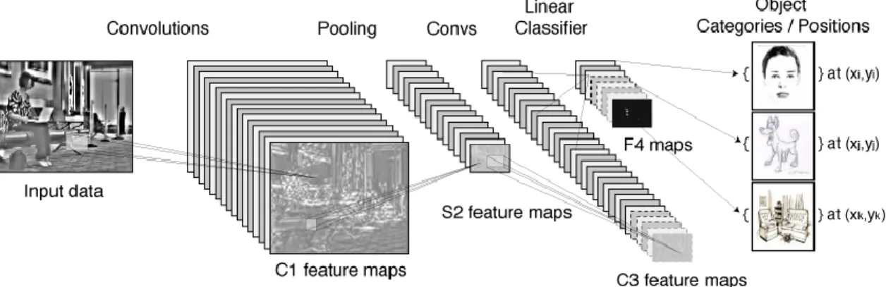
Fully connected layers are the normal flat feed-forward neural network layer. These layers may have a non-linear activation function or a softmax activation in order to output probabilities of class predictions. Fully connected layers are used at the end of the network after feature extraction and consolidation has been performed by the convolutional and pooling layers. They are used to create final non-linear combinations of features and for making predictions by the network. An overview of the use of a CNN is shown in Figure 2.
Figure 3: Convolutional Neural Network Overview. This system takes an input, passes it through a series of convolutional, pooling and linear layers, retrieving an output at the end corresponding to the classification
21
2.5. Model Performance Measurements
Model performance in classification tasks can be measured using the calculation of the 4 different performance measures of the classifier. These are:
1. Accuracy/Classification rate 2. Precision
3. Sensitivity/Recall 4. Specificity
Accuracy refers to the probability that the classification task is performed correctly. Accuracy is measured using the formula:
𝑋 = (𝑇𝑃 + 𝑇𝑁)/(𝑇𝑃 + 𝑇𝑁 + 𝐹𝑃 + 𝐹𝑁),
where X is the precision of the classifier, TP is the true positives, TN is the true negatives, FP is the false positives and FN is the false negatives.
Precision refers to the probability that a diagnostic test is performed correctly, when some classes of images come consecutively. It is a degree of the accuracy measure and is given by the formula:
𝑋 = 𝑇𝑃/(𝑇𝑃 + 𝐹𝑃),
where X is the precision.
Sensitivity is a true positive fraction and is the probability that the classification returns a positive result and is given by:
𝑋 = 𝑇𝑃/(𝑇𝑃 + 𝐹𝑁),
where X is the sensitivity
Specificity is the true negative fraction and refers to the probability that the classification will return negative and is given by:
𝑋 = 𝑇𝑁/(𝑇𝑁 + 𝐹𝑃),
22 Figure 4: Machine learning performance measurement. This shows how true positives and true
negatives are calculated. While also showing false positives and false negatives. The desired outcomes in the classification are true positives and true negatives. Also shown is how precision and
23
2.6. Deep learning and GPU computing
Deep convolutional neural networks have recently been shown to have great power at analysing and classifying data sets, ranging from handwritten digits (MNIST) (LeCun, Bottou, Bengio, & Haffner, 1998), to characters and faces (Strigl, Kofler, & Podlipnig, 2010). Deep neural networks are at their best when big and deep, however in a CPU-based system training these deep neural networks can take weeks, or even months. While these deep neural networks offer significant advantages, they also provide significant limitations in that high data transfer latency limits the ability of multi-CPU and multithreading architectures from expediting the process. In recent years fast parallel neural net code for graphics cards has attempted to overcome this limitation, and has provided results that show image processing techniques can be an order of magnitude faster than the CPU counterpart (Strigl et al., 2010; Uetz & Behnke, 2009). While many of these studies have shown correlation between the application of GPU techniques, the majority of studies are based around high throughput classification of sequences of small images. The scale of improvement that GPU based DNN’s offer in the correct classification of high resolution medical imaging for disease state recognition remains unclear.
In the past, the implementation of GPU computing was a specialised task, requiring a deep understanding of hardware architecture, as problems had to be implemented using graphical API’s such as DirectX and then convert it into a graphical pipeline friendly format. However, with the recent development of CUDA, Nvidia’s GPU programming shell, this process has been simplified immensely. The CUDA programming model has three main key abstractions, hierarchy of thread groups, barrier synchronisation, and shared memories. These abstractions provide fine-grained data parallelism together with task and thread parallelism, forming a type of coarse-grain parallelism (Owens et al., 2007). This means programmers are required to partition problems into independently executed blocks of threads that there are executed in parallel. Each of these threads are able to cooperate when solving each task, and can also be scheduled for execution on any of the available processor cores, either sequentially or concurrently, meaning at specific core is not required to run any program block, greatly speeding the execution of the programme (Vuduc, Chandramowlishwaran, Choi, Guney, & Shringarpure, 2010).
With regards to image classification this “speed up” scales greatly with the size of the dataset. For example, in the field of medical image analysis, a 4-D (3D image over time) CT
24
dataset can require up to 10 GB of memory storage, as it can be in the resolution of 512x512x512x20. For a dataset this large even using high cost massively parallel CPU computing, this process could take several hours. However, using the same GPU acceleration as the ultrasound image, this could be calculated within 10 or 15 minutes (Owens et al., 2008; Pratx & Xing, 2011)f
Traditionally, a high percentage of classification procedures are carried out using Support Vector machines (SVM’s), and much of the research surrounding the field of supervised machine learning involves these techniques (Catanzaro, Sundaram, & Keutzer, 2008a). However, similar research to quantitatively assess the application and cost-benefit of Deep Learning approaches in CNN’s is lacking (Razavian, Azizpour, Sullivan, & Carlsson, 2014).
2.7. Summary
This chapter provided the context for the research, image classification in medical diagnosis. Then several automated approached to image classification were reviewed. The literature explains how image processing is currently being used in the field of medical image diagnosis and what the cutting edge technologies are. A basic explanation was also given of neural networks and support vector machines, which will be used to answer the research question and support or refute the hypotheses given. In the next chapter, an overview of the design of the experimentation will be given.
25
3. Design and Implementation
In this chapter, an overview of the experimental design will be given, along with the specifications of the hardware being used and the data source and contents will be given. The aim of the experiment will also be specified.
All experimentation will be carried out using a desktop PC with an intel i7 5820 processor, a NVidia GTX970 graphics card and 16 gigabytes of on-board RAM.
3.1. Data
The data must be collected and downloaded from the source and cross validated, to ensure the model has enough information to correctly classify the images. The classification procedure will attempt to classify the stages of diabetic retinopathy from images taken of eyes. Data is provided by EyePACS, which is a free platform for retinal screening. The data exploration task will seek to identify the key areas to focus on during research. This includes the identification of features for classification and the feature extraction methodology to be used. Depending on the features selected; colour, texture, shape etc., a different feature extraction technique will be required.
The aim of this project is to solve a complex image processing task, using both CNN and SVM methodologies, taking advantage of Deep Learning techniques where possible, and to investigate both the differences in performance among the different methods, but also to critically assess the relative strengths and weaknesses of the different methodologies. The experimentation will be carried out using a freely assessable EyePACS dataset, consisting of ~30,000 training images of either varying level diabetic retinopathy patients, or NULL cases. This dataset also provides 55,000 test cases, for use after training the model and a master results set, which will provide certainty about the model accuracy. These designs will aim to be as similar as possible to critically assess the strengths of the design, especially in the case of the CNN, however differences will be present despite this as the different frameworks have different requirements in the design process. This process will be contrasted with a support vector machine (SVM) classifier. This type of process was selected due to its status as a more “classic” approach, however it is limited in its ability to handle complex images, therefore the time taken to train the classifier is traditionally large. The process of classification will use a linear SVM. Given an input image, the system first extracts dense local descriptors, which is coded either using local coordinate coding. The codes of the descriptors are then passed to
26
weighted pooling to form a vector for representing the image. Finally, the feature vector is fed to a linear SVM for classification (Catanzaro, Sundaram, & Keutzer, 2008; Lin et al., 2010).
Both of these techniques will be evaluated in the same way, and using the resultant information and the time taking to proceed through the steps we will be able to accept or reject the null hypothesis, as per the experimental overview shown in Figure 1.
3.2. SVM Configuration
The SVM design methodology used the SVM package from the sklearn module in python. This module allowed the classification to proceed without needing too many lines of code. However, it would be difficult to carry out the full classification of the dataset using the SVM technique as it is a resource hungry process and the size and scale of the images, and the dataset itself, suggests that a vast amount of feature and dimensionality reduction would be required before classification could proceed. The method would combine principal component analysis (PCA) along with a reduced size dataset, which was generated from the source images using the supplementary code shown in Appendix 1.
3.3. CNN Configuration
The CNN methodologies proposed here consisted of convolutional neural networks trained with various libraries until a “best performer” was established, using the large colour images, various data augmentation techniques, dynamic resampling for class imbalance between both diseased and non-diseased, which also makes considerations for the different disease states and also a “per patient” feature blending strategy which makes the most of the availability of having two sets of images per patient, which is taken advantage of in the system. The solution to the problem proposed is to use a simple average of blends, consisting of features from two different deep convolutional networks and three sets of weights for each network, forming a robust and powerful classifier. The first implementation of the CNN will begin with the training of the classifier using stochastic gradient decent, using a small weight decay <0.005%. The literature has suggested that this is the correct number to use to ensure the model learns correctly (Krizhevsky, Sutskever, & Hinton, 2012; Liu, Fang, Zhao, Wang, & Zhang,
27
2015). The CNN methodologies proposed here will consist of convolutional neural networks trained with various libraries until a “best performer” is established, using the large colour images, various data augmentation techniques, dynamic resampling for class imbalance between both diseased and non-diseased, which will also make considerations for the different disease states and also a “per patient” feature blending strategy which makes the most of the availability of having two sets of images per patient, again which will be taken advantage of in the system. The solution to the problem proposed will to use a simple average of blends, consisting of features from two different deep convolutional networks and three sets of weights for each network, forming a robust and powerful classifier.
3.4. Summary
This chapter gave an overview of the CNN and SVM experimental process and gave a short description on where the data being used came from. A brief introduction was given to the model design which will be expanded upon in the next chapter. The next chapter will asssess how these methods were implikmented and the results of the model designs that have been implimented, along with any feature or parameter engineering that was required.
28
4. Implementation and Results
In this chapter the implementation and model design of the CNN and SVM models will be shown, along with some findings from the design process that lead to the final models used. A discussion of the different CNN frameworks being tested will be given and an overview of the image processing being imposed on the data prior to model training.
4.1. Image Pre-Processing
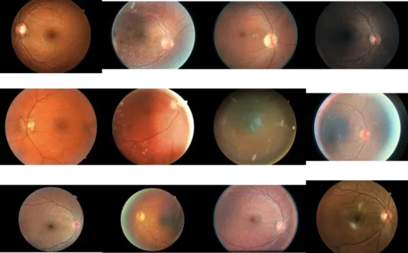
The images in this dataset are too large to be conveniently trained with convolutional networks and even the high end consumer grade hardware that was available to run the process. Therefore, to correctly build a functioning network, a reduction in image size, and therefore performance overhead was required. Since the original images are fairly large (approx. 3000x2000 pixels on average) and most contained a fairly significant black border, the first stage of the development process was to downscale all the images by a factor of five (without interpolation) and trying to remove most of these black borders. The original images are shown in Figure 5, while the resultant images of this processing step are shown in Figure 6. The images were further reduced in size, to squares of 128, 265 and 512 pixels respectively. This gave an even spread of images across multiple file sizes. After this had been completed, background subtraction was used to remove the large black border present in the images.
29 Figure 5: Source training images. This image shows the state of the source images prior to the
pre-processing tasks, including size discrepancies and a large black border being present.
Figure 6: Border Removal. The images from Figure 5, however the black border has been cropped out in this example, and the images have been downscaled by a factor of 5.
To further improve the quality of the resultant training, the images were subjected to further transformations to convince the model that there were many similar images present in
30
the dataset, despite seeming different at face value. The transformations that were carried out are shown below.
These transformations were as follows:
1. The images were cropped with certain probability 2. The images were adjusted for colour balance 3. Adjusting the brightness of the images 4. Adjusting the contrast of the images 5. Flipping some of the images (50% chance)
6. Rotating images by x degrees, somewhere between 0 and 360 7. Equal cropping of X and Y axis
Most of these were implemented from the start. During training random samples are picked from the training set and transformed before queueing them for input to the network. The augmentations were done by spawning different threads on the CPU such that there was almost no delay in waiting for another batch of samples. A collage of the resultant images from this stage is shown in Figure 7.
Figure 7: Collage of Transformed images. This figure shows acollage of 512 x 512 pixel images, which have been cropped and rotated to generate a good field of view.
A resizing transformation was carried out after the cropping and before the other transformations, as it can make some of other operations computationally intensive. This process can be carried out in two different ways:
31
1. Rescale, sparing the original aspect ratio and subsequently carrying out a centre crop on the resulting image
2. Normal bilinear rescaling, however this will destroy the aspect ratio originally present
The method chosen also depends on the model. Early designs focused more on method 1, however during development it was seen that the second method offered some improvements in model performance, therefore the design was revisited. Method 2 was used going forward from here as the best performing models took advantage of this and the addition of another hyperparameter was deemed to be suboptimal as there was a risk of information loss with the centre crops from the first method.
During the training the input is normalised by subtracting the total mean and dividing by the total standard deviation estimated on a few hundred samples before training. After this process was completed, the images were available for testing on the various different models that were highlighted as options to complete this task, broken up between CNN and SVM models.
4.2. Development of SVM
With regards to the SVM methodology, the proposed work was adapted to combat the inherent resource heavy dependency of the SVM classifier. Early approaches sought to classify across the entire dataset, similar to the CNN approach. However, this became unfeasible due to the scope of the used dataset as the vast array of images. Therefore, to correctly build an SVM classifier, a vast reduction in dimensionality was required. To accomplish this, some feature and parameter engineering was required. From the original dataset of 55,000 images, only 3000 could be loaded into an SVM and trained correctly, even with the dimensionality reduction allowed by the engineering tasks. The proposed method consisted of a feature reduction stage and a classification stage using SVM.
For the classification stage we need to extract significant information of each image, encode it as efficiently as possible, and compare one encoded image with a data set using a model encoder based on similarly. Therefore, we have used principal component analysis in order to find the significant features (principal components) of the distribution of the image data set.
32
The basis of principal component analysis is to find the vectors that best account for the distribution of fundus images within the entire image space. This analysis is as follows: Given a training data set of fundus images I1, I2, ..., IM, where every image Ii will be represented as a vector Γi. Then the average fundus image vector Ψ will be calculated as follows:
𝛹 = 1 𝑀 𝑀 𝑖 = 1 (𝛤𝑖)
where each fundus image differs from the average by the vector Γ, i.e. it subtracts the mean fundus image:
𝛷𝑖 = 𝛤𝑖 − 𝛹
This set of very large vectors is then subject to principal components analysis, which seeks a set of M orthonormal vectors un and the eigenvalues (scalars) λk, respectively, which best describe the distribution of the data. The eigenvectors uk and eigenvalues λk are obtained from the covariance matrix C. The λk are the elements in the diagonal of the matrix C.
𝐶 = 1 𝑀 𝑀 𝑛 = 1 𝛷𝑛𝛷𝑇 𝑛 = 𝐴𝐴𝑇 (2)
where the matrix,
𝐴 = [𝛷1𝛷2. . . 𝛷𝑀].
The associated eigenvalues allow us to rank the eigenvectors according to their usefulness in characterizing the variation among the objects (fundus images).
For training the SVM classifier, the Kernel-Adatron technique using a Gaussian kernel was used. To obtain the optimal values for the Gaussian kernel (s) and C we experimented with different SVM classifiers using a range of values. Tenfold cross-validation was applied to find the best classifier based on validation error. The performance of the selected SVMs was quantified based on its sensitivity, specificity and the overall accuracy. In the first experiment, with no restrictions on the Lagrange multipliers (hard margin), we achieved an overall accuracy of 88.6% with 86.2% sensitivity and 90.1% specificity for s=0.3.
33
4.3. Development of CNN
The CNN developments all followed a similar path, the training and test sets came as a subset of the training dataset available as there was a master solution file available with the data. Therefore, any development could be exactly quantified based on ease of use, success rate, time taken to run and development overhead. As there are a great many frameworks available, 2 were selected as potential candidates for testing, Torch and Theano. These models would be generated on a miniaturised dataset, and critically compared to each other, to generate the optimal model for this work
4.3.1. Theano Implementation
The first architecture used was the Theano framework. The network architecture of the Theano designed convolutional network is shown in Figure 8.
34 Figure 8: Theano Network architecture. Shown here is the architecture and positions of the various
layers in the Theano CNN
The networks were trained using rectifier linear units (ReLU), which were used over other activation functions, such as tanh’s or sigmoids, as they can be more easily developed by thresholding the matrix of activations at zero, without suffering from saturation. In some cases, ReLU’s have been shown to greatly accelerate the convergence of gradient descent compared to the other functions, due to the linear form of the function. Unfortunately, ReLU units can be fragile during the training process and can “die”. For example, a large gradient flowing through a ReLU neuron could cause the weights to update in such a way that the neuron will never activate on any data point again. Thus, from that point on, the gradient of that unit will always be zero and can never alter again. With a learning rate set too high, this can be an exponential problem, with a large percentage of the network being dead, causing substantial classification accuracy and implementation difficulties. To combat this, a solution is to use leaky ReLUs, which is one method of overcoming this limitation and fix the “dying ReLU” problem. Leaky RELU’s operate similarly to regular rectifiers, except Instead of the function being zero when x
35
< 0, a leaky ReLU will instead have a small negative slope (usually approx. 0.01). For the purposes of nonlinearity leaky rectifier units are used here following each convolutional and fully connected (dense) layer. The networks were trained with nesterov acceleration with fixed schedule.
For the networks run on the 256 and 128 pixel images, training is stopped immediately after 200 epochs. L2 weight decay is added at a small value, approx. 0.0005, as there are a large number of training examples in the dataset. The problem then becomes a simple regression issue, with mean squared error objective and threshold at (0.5, 1.5, 2.5, 3.5) to obtain integer levels for computing the kappa scores.
As the classes within the dataset are extremely unbalanced, it was difficult to determine the optimal strategy for handling the neural network generation, however the following solution was devised. Initial sampling was carried out across all classes, such that every class was represented equally on average. Gradually, the oversampling of the rarely instances was wound down to give a better view of how the dataset actually appeared. The weights for the resampling between the different disease levels, 0-4 at a given epoch, t, are given as follows:
𝑤𝑖 = 𝑟 𝑡 − 1𝑤0 + (1 − 𝑟 𝑡 − 1 )𝑤𝑓
where r was set at 0.975, w0 were approximately 1.36, 14.4, 6.64, 40.2 and 49.6 and wf were set at 1, 2, 2, 2 and 2. These were all values which were found to work well for initial convergence and final classification. It is probable that an even higher classification accuracy could be achieved by using a dynamically weighted objective function within the theano library, however this was ruled out due to a difficult implementation and unfamiliarity with the minutia of the system architecture.
In this model, the best solution that could be devised was to use 10% of the reduced dataset as a validation set, equating to roughly 590 images from a pool of 5900. The original strategy was to implement and train the network entirely from scratch, however in practice this was deemed too difficult for this particular issue. Instead a smaller network was first trained on the 128 pixel images, which was then used as a base to use the trained weights to initialize partly formed networks of intermediate size which could be implemented on the 256 pixel images. The weights from this were then used to repeat this procedure for the final networks that on the 512 pixel images. The layers of the model were constructed as follows, the 128 px images were used to build layers 1 – 11 and 20 – 25, the 256 px images were used for layers 1 – 15 and 20 – 25, (with the weights of layers 1 – 11 being initialised from the previous weights)
36
and the 512 px images being used for all layers, with weight initialising being the same for the 1 – 11 layers.
Various transformations were carried out at all times during the running of the network. Translation, stretching, rotation, flipping as well as colour augmentation were all dynamically implemented when needed. Each image channel (RGB) was scaled and centred to have zero mean and unit variance over the training set. The output sizes that were generated for the data augmentation pipeline were 112/224/448 pixels for the 128/256/512 pixel input images.
The feature extraction processes were then carried out at the last pooling layer of the convolutional neural networks. Since the feature extraction process was so vital to the success of the training procedure, it is important to increase the quality of the features at this point, to prevent extraction of low quality features. This process was repeated approximately 50 times, with varying s, per image and then mean and standard deviation of each feature is calculated and used as an input for the blending network.
The mean (µ) and standard deviation (σ) of the RMSPool layer output were next extracted for 50 pseudo random transformations for three sets of weights, these being best validation score, best kappa and final weights, for both network a and network b. For each eye, corresponding to each patient, the following were used as the input blending features:
𝑥 = (µ𝑡ℎ𝑖𝑠 𝑒𝑦𝑒, µ𝑜𝑡ℎ𝑒𝑟 𝑒𝑦𝑒, 𝜎𝑡ℎ𝑖𝑠 𝑒𝑦𝑒, 𝜎𝑜𝑡ℎ𝑒𝑟 𝑒𝑦𝑒, 𝛿𝑟𝑖𝑔ℎ𝑡)
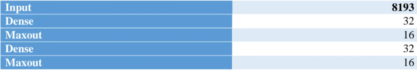
where δ right ∈ {0, 1} was selected as an indicator variable for right eyes. All these features were standardised, and therefore have no mean and unit variance throughout and can therefore be used to train the fully connected network, whose architecture is shown below in Table 1. This is a well understood blend architecture for use in CNN design (Liu, Fang, Zhao, Wang, & Zhang, 2015; Sharif Razavian, Azizpour, Sullivan, & Carlsson, 2014).
Table 1: Theano Blend Network Architecture
Input 8193
Dense 32
Maxout 16
Dense 32
37
4.3.2. Torch Implementation
The first methodology used the Torch and cuDNN libraries for all of the computational work. All work was carried out on the same hardware across all of the different architecture designs using the pre-processed images at the percentage of 10% of the total, by altering the random sample generator script to select this percentage of images. The architecture of the torch model is shown in Figure 9
Figure 9: Torch network architecture. Shown here is the architecture and positions of the various layers in the Torch CNN
The torch model was trained using a clipped MSE error function. This was the standard MSE process, with the output of the model clipped to [0, 4] before evaluation. This was an experiment carried out only for this model as the literature suggested that allowing the model
38
to generate scores lower than zero and greater than 4, would allow for an increased output range, which would assist in separating the different diseased classes. This model also used sigmoid functions, as there was a combination of 4 different sigmoid functions used as the loss. Furthermore, this was used as an opportunity to alter some of the image processing parameters, to assess if the application of GPU computing could increase the speed of the processing calls. This was changed between the Torch and Theano methods as an error exists when attempting to call the WarpAffline function on Theano. The following details were shared by all of our models:
1. Predictions were generated one eye at a time
2. Data transformations were carried out via random affine transformation. It was possible to do these calculations in the GPU, using a dedicated function from NVidia, called WarpAffine. As the GPU is computationally far more efficient than the CPU this increased the speed of these calculations greatly resulted in increased GPU memory usage, but was faster than performing the operations on the CPU. In a typical setup, images were randomly cropped to 85-95%, horizontally flipped, rotated between 0 and 360 degrees and then scaled to the desired model input size
3. Channel-wise global contrast normalization was applied to normalize image color 4. PreLU weight initialization. This was found to help train models with large numbers of
layers
5. Leaky rectifier non-linearities (0.1 leak factor)
In both model cases, the design sought to exploit the fact that each patient, in both training and test datasets, had a left and right eye image present. Therefore, a simple linear model was generated to pool the predictions from both eyes. An early 10% early stopping validation set was reused to fit this model. Several attempts were made unsuccessfully to train a neural network architecture that used both eyes as input. It is possible that further experience with modelling would have allowed this to proceed, however it was abandoned early due to excessive time constraints with both research and implementation.
In the torch model, a similar 10% validation set was used. There were small differences in the layer construction between this and the Theano model as seen in the network architectures in Figs (), however images were used to build layers in a similar way. This model was the first to use PreLU weight initialisation, which was then added into the Theano model,
39
as it was found to help train models that have a large number of layers, and is supported by the literature in this regard (He, Zhang, Ren, & Sun, 2015).
4.4. SVM Implementation
Image pre-processing steps were more advanced for the SVM implementation as a number of feature engineering tasks were required, as the SVM does not have the power of the CNN in terms of easily identifying region of interest (ROI). In this case a number of steps were used, such as gray scale conversion, adaptive histogram equalisation, discrete wavelet transform, PCA and fuzzy C-means clustering for the segmentation task. All image preprocessing tasks at this stage are carried out using the ImageJ processing tool.
4.4.1. Grey Scale Conversion
As all the images are presented in an RGB format, these must be first converted to a grey scale, which is commonly carried out by matching the luminance of the colour image. A greyscale image is an image that only encodes intensity information. The grey scale conversion was carried out using ImageJ’s luminance module. An example image is shown in Figure 10, created using the montage feature of ImageJ.
40 Figure 10: Montage of pre-processed images from the first processing stage, and the resulting
greyscale images.
4.4.2 Adaptive Histogram Equalisation (AHE)
AHE is a technique used to improve the quality of contrast in images, by enhancing the local contrast features of the image. The objective of this method is to define a point transformation, with the assumption that intensity values within the local window are a stoical representation of the distribution of intensity values within the whole image. The point transformation distribution is localised around the mean intensity of the window, covering the entire intensity range present in the image. The result of this AHE is that the dark area in the image that was badly illuminated is brighter in the output, while keeping the areas that were already brightly illuminated the same. The result of this process is shown in Figure 11.
Figure 11: Results of the AHE pre-processing stage. These images show greatly increased local contrast compared to the previous examples.
41
4.4.3. Wavelet Transformation
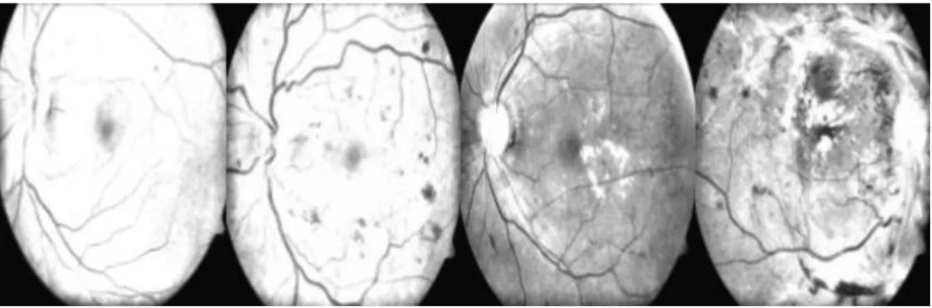
A transformation task changes the representation of the signal without altering the information content of the image. The wavelet transformation is a multi-transformation technique in which different frequencies are used with different resolutions. A discrete wavelet transformation has been seen to yield a fast computation of wavelet transforms, which is easy to implement and reduces the resources required (Priya & Aruna, 2010; Vekkot & Shukla, 2009). The wavelet transform breaks the signal into a set of base functions, called wavelets. These wavelets are obtained from a single wavelet prototype known as the mother wavelet. In this case, the mother wavelet is used to generate all basis functions based on the desired characteristics, in this case the approximation coefficients matrix and details coefficients matrix of input X, where X is a given input image. In this case the haar wavelet is used, and the usage of this transform reduces the size of each image by half. The resultant transformations are shown below in Figure 12.
Figure 12: Results of the wavelet transformation step of the feature engineering stage
4.4.4. Principal Component Analysis
PCA was used next to make a classifier system more effective, as discussed previously. Prior to the classification step, a dimensionality reduction stage was required. The PCA task is based on the assumption that most information about classes is contained in the directions along which the variations are the largest. There is an assumption made for feature extraction and dimensionality reduction by PCA, that most information of the observation vectors is contained
42
in the subspace spanned by the first m principal axes, where m < p, where p is the dimension of the dataset and m is the principal axis.
4.4.5. Fuzzy
c
-Means Clustering
FCM is a clustering method that allows one price of data to belong with multiple clusters. Upon investigation of the literature, it was decided to focus on a c means method as it has been shown in medical diagnostic systems that this can outperform a harder k means method. In this case, the clustering is based around detecting blood vessels that can be used to grade the severity of the disease. The clustering is carried out by detecting the blood vessels in the eye images and grouping these to one category as pixels which are turned on, and all other pixels, which are turned off. The results of this process are shown below in Figure 13.
Figure 13: Results of the application of fuzzy c-means clustering to the sample images
4.4.6. Feature Extraction
After these stages have been completed, the feature extraction stage is carried out, which extracts information from the image to use as inputs into the SVM. These features include
1. Area of on pixels: The area of white pixels remaining in the image 2. Mean: the average distribution of all pixels divided by the original values
3. Standard Deviation: The square of every pixel of all individual samples is collected and then an average across these N samples is calculated
43
After the processing steps have been completed, the SVM algorithm is used to produce the classification parameters for the calculated features that have been derived from the processing stages. The algorithm should break down the images into their respective classes based on level of disease state. In this case, the image is considered to be classified correctly if the fundus of the image is actually abnormal and has been screened as abnormal. The goal of the SVM here is to find the optimal hyperplane that separates the clusters of vectors in such a way that the cases with one characteristic are on one side of the plane and those without are on the other. In this case, diseased vs. non-diseased, then further separated based on the severity of the condition. The SVM makes use of a function called a kernel function, which maps the data into a different feature space where the hyperplane can be used to do the separation task
4.5. Summary
In this section the implementation of the image pre-processing steps, along with the development and implementation of the various models was discussed. Various feature and parameter engineering steps required were covered in detail and the stepwise process for how each classification would proceed was also discussed. As shown below in Table 2, there were various different stages involved in all the different methodologies before the models were fully developed, showing the breadth of options available for each technique and the level to which they were implemented in this case.
44 Table 2: Summary of the various models being investigated and the parameter and feature
engineering tasks involved with their development. Techni
ques
Framew orks
Parameter Engineering Feature Engineering
CNN Theano Decoding alterations None; features were extracted at last pooling layer
Rectifier unit design Batch Normalisation Layer modelling
Torch Clipped MSE Function None; features were extracted at last pooling layer
Random Affine Transformations Pre-Lu Weight initialisation
SVM Scikit - Learn
Reduction in image data to ensure model functionality Grey-scale conversion Adaptive Histogram Equalisation Discrete Wavelet Transformation
Principal Component Analysis Fuzzy C-means Clustering