ROC-based cost-sensitive classification with a reject option

HAL Id: hal-02088187

https://hal-normandie-univ.archives-ouvertes.fr/hal-02088187

Submitted on 2 Apr 2019

HAL

is a multi-disciplinary open access

archive for the deposit and dissemination of

sci-entific research documents, whether they are

pub-lished or not. The documents may come from

teaching and research institutions in France or

abroad, or from public or private research centers.

L’archive ouverte pluridisciplinaire

HAL

, est

destinée au dépôt et à la diffusion de documents

scientifiques de niveau recherche, publiés ou non,

émanant des établissements d’enseignement et de

recherche français ou étrangers, des laboratoires

publics ou privés.

ROC-based cost-sensitive classification with a reject

option

Clément Dubos, Simon Bernard, Sébastien Adam, Robert Sabourin

To cite this version:

Clément Dubos, Simon Bernard, Sébastien Adam, Robert Sabourin. ROC-based cost-sensitive

clas-sification with a reject option. 23rd IEEE International Conference on Pattern Recognition (ICPR),

Dec 2016, Cancun, Mexico. �10.1109/ICPR.2016.7900146�. �hal-02088187�

ROC-based cost-sensitive classification with a reject

option

Cl´ement Dubos

,Simon Bernard

,S´ebastien Adam

,Robert Sabourin

†_{Laboratoire d’Imagerie, de Vision et d’Intelligence Artificielle,} ´

Ecole de Technologie Sup´erieure, Universit´e du Qu´ebec, Montreal, Canada [email protected]

Abstract—In many real-world classification tasks, such as med-ical diagnosis, it is crucial to take into account misclassification costs for designing an accurate classification system. Nevertheless, begin able to reject a sample is also often needed in order to avoid a very risky prediction error. In that case, a cost-sensitive classi-fier must embed a rejection mechanism, that takes into account the rejection costs as well as the misclassification costs. In binary classification, the ROC space has shown to be very powerful for designing cost-sensitive classifiers, but it has been poorly exploited for designing classifiers able to reject. The purpose of this work is to extend a ROC-based ensemble method recently proposed, called the ROC Front method, with a cost-sensitive rejection mechanism. This approach compares favorably to the state-of-the-art ROC-based rejection rule recently proposed for binary cost-sensitive classification. It is also more robust as it allows to design an accurate classifier for all cost-sensitive situations contrary to the state-of-the-art method that fails in many cases, as for example with small datasets.

I. INTRODUCTION

Many real-world classification problems naturally exhibit imbalanced misclassification costs. Medical diagnosis is a typical example for which predicting a healthy condition for a patient who actually suffers from a serious pathology is obviously more dangerous than the opposite situation. For such cases, a wide variety of classifiers exist that take into account some predefined costs, associated to each of the possible classification errors. However, even by focusing on specific types of error, at the expense of the others, it may be difficult to completely avoid very costly prediction errors. In the previous example of medical diagnosis, one single diagnosis error can imply very serious consequences. In such a situation, it is desirable to be able not to predict any of the healthy/pathological classes, instead of taking the risk to predict ’healthy’ instead of ’pathological’. Consequently, in addition to cost-sensitivity, classifiers must be able to reject a sample when the risk of being wrong is critical.

In the cost-sensitive binary classification framework, the

Receiver Operating Characteristic(ROC) space has shown to be very powerful for dealing with imbalanced misclassification costs ([1]). The reason is that it allows to describe the performance of binary classifiers at different operating points, i.e. considering different cost ratios. However, it has been poorly exploited for incorporating a reject option in the cost-sensitive framework. The main reason is that the ROC space

does not naturally allows to consider the reject option as a third possible outcome of binary classifiers.

Consider a binary classification task, where a classifier predicts either the positive (P) or the negative (N) class. In a cost-sensitive framework, the misclassification costs are defined in a matrix, as shown in Table Ia. When adding the ability to reject, a third column has to be defined for the cost of rejecting samples from each of the two classes, as shown in Table Ib. The traditional 2D ROC space allows the TABLE I: Cost matrices definition. CF N denotes the cost

of predicting negative instead of positive, CF P the cost of

predictingpositive instead ofnegative,CT P andCT N are the

profits associated to correct predictions, andCRP (resp.CRN)

denotes the cost of rejecting apositive(resp.negative) sample.

(a) Traditional Cost Matrix

ˆ

P Nˆ P CT P CF N

N CF P CT N

(b) Cost Matrix with a reject option

ˆ

P Nˆ Rˆ P CT P CF N CRP

N CF P CT N CRN

representation of a classifier ability to handleCF P andCF N.

Nevertheless, if one wants to transpose the ROC space in the Table Ib case, he will have to add 2 more dimensions, corresponding to CRP andCRN.

As far as we know, very few works have proposed a reject-based extension of the ROC space ([2], [3]). In both [2] and [3], a third dimension, related to the rejection performance, is added to the regular 2D ROC space. In the first work ([2]), this third dimension represents the ability of an operating point to reject a sample predicted with a low confidence. However, it does not allow to take into account cost matrices like the one in Table Ib, since two more dimensions are needed to separately consider CRP andCRN, instead of just one.

In the second work ([3]), the third dimension represents the rates of samples predicted as positive whereas they are expected to be rejected. This extended ROC space is used for outlier detection, where samples are classified either as

positive or negative whereas they may actually belong to a third unseen class. This case would correspond to adding a new row in the Table Ia, instead of a new column as it is the case in our context.

Tortorella proposes in [4] another type of ROC-based re-jection mechanism. The traditional 2D ROC space is used to design a reject rule that leans on two decision thresholds applied on the binary classifier outcomes. It has been shown in [5] that this method is theoretically equivalent to the optimal Chow’s reject rule proposed in [6], for binary classification. However this method is ineffective in two types of situation: (i) when the Equation 8 is not true (cf. Section II) and (ii) when the dataset used for the ROC analysis is too small to correctly estimate the ROC curve. In that case, the two decision thresholds are most of the times equals and irrelevant. In a recent paper ([7]), we have shown that, for cost-sensitive classification, it can be more efficient to exploit the ROC space for learning a pool of classifiers, instead of only focusing on the decision thresholds proposed in the ROC curve of a single classifier. The purpose of the present work is to extend the method in [7] with a rejection mechanism that is able to jointly take into account the misclassification and rejection costs as defined in the Table Ib. The proposed method shows a significant improvement over the Tortorella’s method, and allows to give an accurate cost-sensitive solution in all cases, in particular when the dataset is small.

The rest of the paper is organized as follows: the next sec-tion explains the Tortorella’s method for designing a reject rule thanks to a ROC analysis; Section III presents the proposed approach; and Section IV details the experimental comparison between both methods, i.e. Tortorella’s reject rule and our approach.

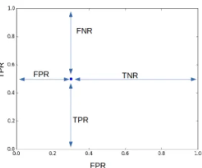
II. ROC-BASED REJECT RULE(TORTORELLA’S METHOD) A natural way to make any binary classifier cost-sensitive is to optimize a decision threshold on its outcome, according to a given cost matrix. This allows to train the classifier regardless the costs, and to find the decision threshold that best suits to the misclassification costs afterwards. To do so, the ROC space is often used, since it allows to represent any binary classification system via its ability to recognize both classes: the first class through the True Positive Rate (TPR) and the second class through the False Positive Rate (FPR). Such a classification system, that gives a predictionyˆfor any instance x, will be represented in the ROC space by a 2D point, as illustrated in Figure 1.

Consider now that a classifier gives an output scoreh(x)on any instancex. For having a predictionyˆ, a thresholdthas to be set onh(x), such that yˆ=P if h(x)> t,yˆ=N else. A typical way to represent the performance of such a classifier in the ROC space is to consider all the possible thresholds, and to draw the corresponding ROC curve, as illustrated on Figure 2. In that way, it is easy to find the operating point of this curve (and thus the corresponding threshold t) that best suits to given misclassification costs. This is usually achieved using iso-performance lines ([8]) defined by a slope given by

m= p(N)CF P

p(P)CF N

(1)

Fig. 1: Representation of a classifier system in the ROC space. F P R,T P R,F N RandT N Rrespectively denotes the false positive, true positive, false negative and true negatives rates.

Fig. 2: ROC curves and iso-performance lines

where, p(P) and p(N) are the prior probabilities of the

positive and the negativeclasses. The best threshold is given by the operating point for which the iso-performance line is tangent to the ROC curve, as illustrated in Figure 2.

The idea behind the method proposed in [4], denotedRBR hereafter, is to extend the iso-performance line principle for finding two decision thresholds,t1 andt2, in such a way that

the final predictionyˆis defined by:

ˆ y=      P if h(x)> t1 R if t2< h(x)< t1 N else (2)

These thresholds t1 and t2 can be find using two

iso-performance lines, the slopes of which are: m1=−

p(N)C_{T N}0

p(P)C_{F N}0 and m2=−

p(N)C_{F P}0 p(P)C_{T P}0 (3) whereC_{T N}0 ,C_{F N}0 ,C_{F P}0 andC_{T P}0 are modified costs, as:

C_{T N}0 =CT N −CRN (4)

CF P0 =CF P −CRN (5)

C_{F N}0 =CF N−CRP (6)

C_{T P}0 =CT P −CRP (7)

The threshold t1 (resp. t2) is found with the m1 (resp. m2)

Note that there are cases for which it is not possible to find two consistent thresholds t1 andt2. When determining both

values, three different situations can be encountered: 1) t1< t2

2) t1=t2

3) t1> t2

In the second and third situations, the prediction function of Equation 2 can not be applied. In that case, Tortorella suggests in [4] not to perform any rejection, and to use instead the regular method with only one threshold. Two types of situations can led to these situations: (i) when Equation 8 is not true and (ii) when the dataset is too small. For further explanations, please see [4].

C_{T N}0 C_{F N}0 >

C_{F P}0

C_{T P}0 (8)

III. REJECTING WITHROC-BASED COST-SENSITIVE CLASSIFIERS

In [9], [7], we have proposed an ensemble method for cost-sensitive classification, called the ROC Front method. The rationale behind this method is to replace the traditional de-cision parameter optimization by a model selection approach, based on an ensemble of cost-sensitive classifiers optimized in the ROC space. This approach has shown to significantly improve the cost-sensitive results over the decision parameter optimization approach. The goal of the method proposed in this paper is to extend this ROC-based model selection with a rejection mechanism.

What is called ROC Front is an ensemble of diverse cost-sensitive classifiers, that proposes a variety of solutions that suit to different cost-sensitive scenarios. When a cost matrix is considered, the most suitable classifier is selected accordingly in this ensemble. For adding a reject option, a second stage is added, composed with the following steps:

1) All pairs of classifiers from the ROC front are generated. Each pair of classifiers Hij = (hi, hj) is used as a

combining classifier such that the prediction is obtained following the decision function:

ˆ y=      P if hi(x) =P and hj(x) =P N if hi(x) =N and hj(x) =N R else (9)

2) These Hij classifiers are projected in a 4D ROC space,

where the dimensions correspond to the T P R, F P R, RP R andRN R, whereRP R andRN R stand for the rejected positive rates and rejected negative rates. In that extended ROC Space, the pointPo of coordinates

(1,0,0,0)corresponds to a classifier that always predicts the correct class for any new instance, and that never reject. Any other points of this space is a particular cost-sensitive classifier, represented by its 4 rates (T P R, F P R,RP R,RN R). The closer toPo, the more

accu-rate this classifier will be. However, as for the ROC Front method, the goal here is to obtain a diverse pool of classifiers, well spread all across the 4D ROC space.

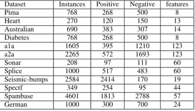
Dataset Instances Positive Negative features

Pima 768 268 500 8 Heart 270 120 150 13 Australian 690 383 307 14 Diabetes 768 268 500 8 a1a 1605 395 1210 123 a2a 2265 572 1693 123 Sonar 208 97 111 60 Splice 1000 517 483 60 Seismic-bumps 2584 2414 170 19 Spectf 349 254 95 44 Spambase 4601 1813 2788 57 German 1000 300 700 24

TABLE II: Datasets

3) Among all the Hij classifiers, a new 4D ROC Front

is built with the non-dominated solutions, in the sense of Pareto-domination as defined in the multiobjective optimization literature (please see [10] for a formal definition of Pareto-domination). In practice, this means that theHijclassifiers that can never be considered to be

the best solution for at least one cost-sensitive scenario, are discarded from the 4D ROC Front.

This ROC Front variant, with reject option, is denotedRF R in the following.

Finally, when a given cost matrix is considered, the model selection process is applied in the same way it is done in [9], [7], that is to say by minimizing the loss function defined by:

L(Hij, D) =p(P)   X j=1..3 C1jR1j  +p(N)   X j=1..3 C2jR2j   (10) whereDis a dataset,C1j (resp.C2j) corresponds to the costs

in the first (resp. second) row of the Table Ib matrix, andR1j

(resp.R2j) are the corresponding rates, estimated on D. For

example,C11 isCT P in Table Ib, andR11 is the true positive

rate ofHij, estimated on D.

IV. EXPERIMENTS

A. Experimental protocol

For evaluating both the RBR and RF R methods, SVM classifiers with a Radial Basis Function (RBF) Kernel have been used as base classifiers. The reason of this choice is that these classifiers are naturally cost-sensitive through their 3 hyperparameters: γ, C+ _{and C}− _{(please see [7] for} additional explanations on these hyperparameters). By tuning these values, in particular C+ _{and C}−_{, one can make such} an SVM classifier suits to given misclassification costs. As a consequence, the ROC front is made up with an ensemble of SVM classifiers, all trained with different triplets of hyperpa-rameters(γ, C+, C−). In the whole experiments, all the SVM has been implemented via the LibSVM software ([11]).

As for the experimental protocol, it has been inspired by the protocol used in [4]. First,12datasets have been selected from the UCI repository ([12]), and are described in Table II. For both methods, an independent validation set is required for finding thet1andt2inRBR, and for evaluating and selecting

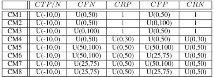
CT P /N CF N CRP CF P CRN

CM1 U(-10,0) U(0,50) 1 U(0,50) 1

CM2 U(-10,0) U(0,50) 1 U(0,100) 1

CM3 U(-10,0) U(0,100) 1 U(0,50) 1

CM4 U(-10,0) U(0,50) U(0,30) U(0,50) U(0,30) CM5 U(-10,0) U(50,100) U(0,50) U(50,100) U(0,50) CM6 U(-10,0) U(50,100) U(0,50) U(25,75) U(0,50) CM7 U(-10,0) U(25,75) U(0,50) U(50,100) U(0,50) CM8 U(-10,0) U(25,75) U(0,50) U(25,75) U(0,50)

TABLE III: Cost Models. U denotes a uniform random selec-tion in the corresponding interval of values. CM1 to CM4 are excerpt from [4]. In these first 4 CM, CRP is always equal

toCRN, while in CM5 to CM8, different values of CRP and

CRN can be obtained.

the pairs of classifiers in RF R. For that reason, each datasets have been divided into 3 distinct subsets, with 60% of the instances in the training set Dr, 20% in the validation set

Dv, and the remaining 20% in the test setDs. For reliability

concerns, 10 random partitions of each dataset have been considered in the whole experiments.

Second, several cost matrices have been generated. For that purpose, eight types of cost matrices, called cost models (CM), have been considered. Each of these CM represents a typical imbalanced costs scenario. The first four CM are excerpt from the experimental protocol proposed in [4]. The last four CM are additional CM we propose to extend the analysis: none of the CM proposed in [4] correspond to situations where the reject costs are potentially imbalanced. However, it is an important feature in our context, since it may be important to focus on the rejection of one class of instances, rather than the other. Thus, it is desirable not to reject too much instances from the healthy class. As a consequence, the four additional CM propose situations where CRP and CRN are

potentially imbalanced. In addition to this, these CM present a wider variety of imbalanced costs situations, with (i) both misclassification costs always higher than reject costs (CM5), (ii) one misclassification always higher than reject costs (CM6 and CM7) and (iii) potentially balanced misclassification costs (CM8). Table III summarizes the definition of these 8 cost models.

Each of these CM have been used to generate 1000 random cost matrices, leading to a total of 8 ×1000 = 8000 cost matrices. For each of them, results are averaged over the 10 random partitions described above. Consequently, both methods have been evaluated over 10×8000 = 80000 runs for each dataset.

Concerning the RBRmethod, a single SVM classifier has been trained onDr, for which the hyperparameters have been

chosen according to a classical grid search procedure, as proposed in the LibSVM ([11]). Then, the thresholdst1andt2

have been selected with the validation setDv. And finally, the

resulting classifier has been evaluated on Ds, by computing

the cost-sensitive loss defined in Equation 10.

As for the RF R method, the ROC Front has been built on Dr, as explained in [9], [7]. The pool of classifier

combinations, made up with the pairs of classifiers from this ROC front, is then evaluated on Dv, through a 5-fold

cross-validation (CV) procedure. As a result, each combi-nation is represented in the extended 4D ROC space by a

(T P R, F P R, RP R, RN R) point, each of these coordinates being averaged over the5 folds of the CV procedure. Details are given by the Algorithm 1.

This algorithm takes as input a ROC Front, represented by an ensemble of hyperparameter vectors(γ, C+, C−), each of which corresponding to one particular SVM classifier. Firstly, the 5-fold cross-validation is prepared, by recording the pre-dictions of all the classifiers from the ROC Front, on all the5

folds (line1to7). Secondly, all the possible pairs of classifiers from the ROC Front are generated (line 8). Thirdly, for all these pairs of classifiers, new predictions are given for each folds of the CV procedure, applying the decision rule given in Equation 9 (line9to23). These predictions are used to build a mean confusion matrix, averaged over the rates obtained on the5 folds. The projection of any combining classifier of the RF Rmethod in the extended 4D ROC space, is excerpt from this mean confusion matrix. Finally, the algorithm outputs the ”best” combining classifiers in this ROC space, in the sense of Pareto-domination, as explain in Section III (line24).

When the cost matrix is then considered, the most suitable pairs is selected by minimizing the loss function of Equation 10, also estimated on Dv. Finally, the resulting combining

classifier has been evaluated onDs, as for theRBRmethod. B. Results

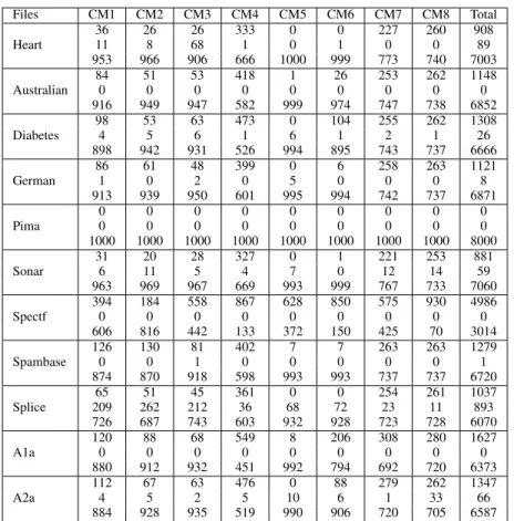
In order to assess the significance of the results, the Wilcoxon signed ranks test has been applied on each cost matrix evaluation, as in [4] and as recommended in [13] for comparison of two classifiers. Consequently, each CM, applied on each dataset, have led to 1000 significant win/loss results, obtained over the 10 random partitions. These results are gathered in Table IV. Each cell of Table IV contains 3 values: from the top to the bottom, the significant win counts for the RF Rmethod, the significant loss counts and the number of cost matrices for which both methods do not give loss results significantly different. For exhaustiveness, we also report in the last column, the total counts of win/loss/tie counts, over the8000 matrices.

The first observation made from this table is thatRF Rand RBR do not give statistically different results in a majority of cases, i.e.80.9%(71216of the88000comparisons). Then, RF Rsignificantly outperformsRBRfor17.78%of the cases (15642over88000), whileRBRrarely outperformsRF R, i.e. for 1.3% of the cases only (1142over 88000). To sum it up, the proposed approach is at least as accurate as the Tortorella’s approach, and gives a significant improvement for more than1

out of6 cases, and so for a wide variety of imbalanced costs. A strong advantage of the RF R method is that it never fails to give a suitable cost-sensitive solutions, whatever the priors and the costs. On the contrary, as explained at the end of Section II, it is sometimes impossible for theRBRapproach

Files CM1 CM2 CM3 CM4 CM5 CM6 CM7 CM8 Total 36 26 26 333 0 0 227 260 908 Heart 11 8 68 1 0 1 0 0 89 953 966 906 666 1000 999 773 740 7003 84 51 53 418 1 26 253 262 1148 Australian 0 0 0 0 0 0 0 0 0 916 949 947 582 999 974 747 738 6852 98 53 63 473 0 104 255 262 1308 Diabetes 4 5 6 1 6 1 2 1 26 898 942 931 526 994 895 743 737 6666 86 61 48 399 0 6 258 263 1121 German 1 0 2 0 5 0 0 0 8 913 939 950 601 995 994 742 737 6871 0 0 0 0 0 0 0 0 0 Pima 0 0 0 0 0 0 0 0 0 1000 1000 1000 1000 1000 1000 1000 1000 8000 31 20 28 327 0 1 221 253 881 Sonar 6 11 5 4 7 0 12 14 59 963 969 967 669 993 999 767 733 7060 394 184 558 867 628 850 575 930 4986 Spectf 0 0 0 0 0 0 0 0 0 606 816 442 133 372 150 425 70 3014 126 130 81 402 7 7 263 263 1279 Spambase 0 0 1 0 0 0 0 0 1 874 870 918 598 993 993 737 737 6720 65 51 45 361 0 0 254 261 1037 Splice 209 262 212 36 68 72 23 11 893 726 687 743 603 932 928 723 728 6070 120 88 68 549 8 206 308 280 1627 A1a 0 0 0 0 0 0 0 0 0 880 912 932 451 992 794 692 720 6373 112 67 63 476 0 88 279 262 1347 A2a 4 5 2 5 10 6 1 33 66 884 928 935 519 990 906 720 705 6587

TABLE IV: Results of the comparison as win/loss/tie counts over the8×11 = 88000cost matrices

Files CM1 CM2 CM3 CM4 CM5 CM6 CM7 CM8 Heart 22 16 22 25 0 0 0 0 Australian 58 23 38 108 0 25 0 0 Diabetes 75 30 52 163 0 104 1 0 German 52 22 31 86 0 5 5 1 Pima 0 0 0 0 0 0 0 0 Sonar 15 10 23 22 5 1 13 13 Spectf 240 114 155 541 577 776 323 653 Spambase 63 41 37 84 0 7 0 0 Splice 50 32 35 55 3 11 0 0 A1a 96 52 56 238 8 206 54 18 A2a 89 45 53 171 8 94 26 33

TABLE V: Counts of cost matrices for which a 0-reject classifier has been used in replacement of theRBRmethod

to find consistent thresholds such that t1 < t2. Every time

such a situation has been encountered in our experiments, a

0-reject classifier has been used instead, with only one decision threshold tused, and found by minimizing the loss function. The number of cases for which theRF Rmethod is compared to the0-reject classifier in replacement of theRBRmethod are summarized in Table V. These counts confirm the conclusion of Tortorella in [4]: it is more likely with the cost model CM4 than with the cost models CM1 to CM3, that the condition for finding the thresholdst1 andt2, expressed by Equation 8, are

not met.

Another interesting observation made from this table is that RBRoften fails to find a consistent pair of threshold (t1, t2)

for the Spectf dataset. From our point of view, it highlights another drawback of the method: when there is only few

validation instances available, which is the case of theSpectf

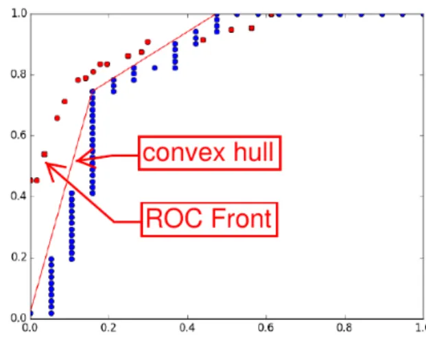
dataset due to the low number of negative instances, the ROC curve does not contain a sufficient number of operating points to propose enough different cost-sensitive solutions. This is well illustrated in Figure 3, which represents the ROC curve of the classifier used in theRBRmethod for theSpectfdataset (the blue points). The potentially selected operating points for any cost-sensitive scenarios are the points lying on the red curve, called the convex hull. One can see that only 4 points are available here. In that case, it is likely that the same operating point will be selected for both thresholds. This pathological case is also discussed in [4]. On the opposite, the corresponding ROC Front used inRF R, made up with several cost-sensitive classifiers (the red points), proposes a lot more diverse ensemble of solutions. The reason is that the number of

Algorithm 1 ROC Front with reject option (RF R)

Require: Dv : a Dataset

Require: F : the number of folds for the cross-validation (CV) procedure

Require: Θ ={θi, i= 1..K}: a pool of K triplets of

hyperparam-eters, composing the ROC Front, whereθi= (Ci+, C

−

i , γi)

Data Ω ={(θi, θj), i, j = 1..K, i ≥j} : a pool ofK(K+ 1)/2

pairs of classifiers fromΘ

Data Tn: the nthfold of CV procedure applied onDv, with n=

1..F

Data Pn,i,j : the prediction of theithclassifier, on thejthinstance

of thenthfold

Data Confn,i : the confusion matrix of the ith classifier, obtained

on thenth_fold

Function P artitionF orCV(Dv, F) : outputs F distincts folds

following a classical CV procedure.

Function T rain(θ, T) : outputs a classifier trained on the dataset

T, with theθ hyperparameter values.

Function P redict(θ, T) : outputs the prediction of a given SVM classifierθfor all the instances inT

Function bestCombiningClassif(Conf,Ω) : outputs the subset of Ω that represent the best solutions in the multiobjective optimization sense (Pareto optimality).

Ensure: Γ ={(θi, θj), θi, θj∈Ω}: the ensemble of pairs of SVM

classifiers, composing theRF Rensemble.

1: Tn=1..F ←P artitionF orCV(Dv, F) 2: fori from 1 to Kdo 3: forn from 1 to Fdo 4: ϑ←T rain(θi,∪Fs=1,s6=nTs) 5: Pn,i,.←P redict(ϑ, Tn) 6: end for 7: end for 8: Ω← {(θi, θj), θi, θj∈Θ, i, j= 1..K, i≥j} 9: fori=1..Kdo 10: forj=i..Kdo 11: forn from 1 to Fdo 12: forp from 1 to|Tn|do 13: ifPn,i,p6=Pn,j,p then 14: P rejectp←Rejection 15: else 16: P rejectp←Pn,j,p 17: end if 18: end for

19: Confn,.←Conf usionM atrix(Tn, P reject)

20: end for

21: Conft←mean(Confn,.)

22: end for 23: end for

24: Γ←bestCombiningClassif(Conf.,Ω)

these classifiers does not depend on the number of validation instances available. This explains the particularly good results of RF Ron the Spectf dataset, as shown in Table IV.

V. CONCLUSION

In this paper, a ROC-based ensemble method has been proposed for cost-sensitive classification with rejection. This method relies on a pool of cost-sensitive classifiers, called the ROC Front. Pairs of classifiers from the ROC Front are com-bined to add the ability to reject. The combining classifiers that proposes the best solution for tackling particular cost-sensitive situations, i.e. with given (imbalanced) misclassification and

Fig. 3: Illustration of the pathological case forRBR, where the ROC curve does not contain enough operating points for selecting two differents thresholds

rejection costs, are retained to compose a new ROC Front with reject option.

The proposed approach compares favorably to the state-of-the-art ROC-based reject rule, with two noticeable improve-ments: (i) it gives a significant improvement in terms of cost-sensitive performance and (ii) it is always able to propose an efficient solution for any cost-sensitive situation, contrary to the state-of-the-art method that regularly fails to introduce the reject option regarding the costs ratios.

REFERENCES

[1] T. Fawcett, “An introduction to roc analysis,” Pattern Recognition Letters, vol. 27, no. 8, pp. 861–874, 2006.

[2] S. Alsing, E. Blasch, and K. Bauer, “Three-dimensional receiver op-erating characteristic (roc) trajectory concepts for the evaluation of target recognition algorithms faced with the unknown target detection problem,” pp. 449–458, 1999.

[3] T. Landgrebe, D. Tax, P. Paclk, and R. Duin, “The interaction between classification and reject performance for distance-based reject-option classifiers,”Pattern Recognition Letters, vol. 27, pp. 908–917, 2006. [4] F. Tortorella, “A roc-based reject rule for dichotomizers,”Pattern

Recog-nition Letters, vol. 26, no. 2, pp. 167–180, 2005.

[5] C. Santos-Pereira and A. Pires, “On optimal reject rules and roc curves,” Pattern Recognition Letters, vol. 26, no. 7, pp. 943–952, 2005. [6] C. Chow, “On optimum recognition error and reject tradeoff,” IEEE

Transactions on Information Theory, vol. 16, no. 1, pp. 41–46, 1970. [7] S. Bernard, C. Chatelain, S. Adam, and R. Sabourin, “The multiclass

roc front method for cost-sensitive classification,”Pattern Recognition, vol. 46, pp. 46–60, 2016.

[8] F. Provost and T. Fawcett, “Robust classification for imprecise environ-ments,”Machine Learning, vol. 42, no. 3, pp. 203–231, 2001. [9] C. Chatelain, S. Adam, Y. Lecourtier, L. Heutte, and T. Paquet, “A

multi-model selection framework for unknown and/or evolutive misclassifica-tion cost problems,”Pattern Recognition, vol. 43, no. 3, pp. 815–823, 2010.

[10] K. Deb,Multi-Objective Optimization Using Evolutionary Algorithms. New York, NY, USA: John Wiley & Sons, Inc., 2001.

[11] C. Chang and C. Lin, “Libsvm: A library for support vector machines,” ACM Transaction on Intelligent Systems and Technology, vol. 2, no. 3, pp. 1–27, 2011.

[12] K. Bache and M. Lichman, “UCI Machine Learning Repository,” 2013. [Online]. Available: http://archive.ics.uci.edu/ml

[13] J. Demsar, “Statistical comparisons of classifiers over multiple data sets,” Journal of Machine Learning Research, vol. 7, pp. 1–30, 2006.