Semantic segmentation of outdoor scenes using LIDAR cloud point

POURIA BABAHAJIANI

SEMANTIC SEGMENTATION OF OUTDOOR SCENES USING LIDAR CLOUD POINT

Master of Science thesis

Examiner: Professor Hannu Eskola, Professor Moncef Gabbouj and Dr Lixin Fan

Examiner and topic approved in the Natural Science Faculty Council meeting on 30th July 2014

Major: Medical Informatics Major: Biomedical Engineering

Examiner: Professor Hannu Eskola, Professor Moncef Gabbouj, Dr Lixin Fan

Keywords: 3D point cloud, LiDAR, classification, segmentation, image alignment, street view, feature extraction, machine learning, Mobile Laser Scanning

In this paper we present a novel street scene semantic recognition framework, which takes advantage of 3D point clouds captured by a high definition LiDAR laser scanner. An important problem in object recognition is the need for sufficient labeled training data to learn robust classifiers. In this paper we show how to significantly reduce the need for manually labeled training data by reduction of scene complexity using non-supervised ground and building segmentation. Our system first automatically segments grounds point cloud, this is because the ground connects almost all other objects and we will use a connect component based algorithm to over segment the point clouds. Then, using binary range image processing building facades will be detected. Remained point cloud will grouped into voxels which are then transformed to super voxels. Local 3D features extracted from super voxels are classified by trained boosted decision trees and labeled with semantic classes e.g. tree, pedestrian, car.

Given labeled 3D points cloud and 2D image with known viewing camera pose, the proposed association module aligned collections of 3D points to the groups of 2D image pixel to parsing 2D cubic images. One noticeable advantage of our method is the robustness to different lighting condition, shadows and city landscape. The proposed method is evaluated both quantitatively and qualitatively on a challenging fixed-position Terrestrial Laser Scanning (TLS) Velodyne data set and Mobile Laser Scanning (MLS), NAVTEQ True databases. Robust scene parsing results are reported.

PREFACE

This Master of Science Thesis has been carried out in the Department of Biomedical En-gineering at Tampere University of Technology (TUT), Tampere, Finland as a part of Nokia s project during June 2012 – March 2014. I am pleased to express my gratitude to my thesis supervisors, Professor Hannu Eskola, Professor Moncef Gabbouj and Dr Lixin Fan for their valuable guidance and support throughout the thesis period. I would also like to express my appreciation to my seniors, Viktor Vad and Junsheng Fu and who have worked in the same project. Their way of sharing knowledge and willing to help attitude has supported me a lot to foster my work in the correct direction. I am also grateful to Esin Goldugan, You Yu, Kimmo Roimela from Nokia Company for their valuable com-ments and suggestions regarding our results.

Finally, it is a pleasure to thank my family for their support and motivation to pursue this Master’s degree.

Feb, 2014

2.2 Feature extraction ... 6

2.3 Segmentation and classification of 3D Data ... 7

2.3.1 Segmentation of 3D point cloud ... 7

2.3.2 Classification of 3D Data ... 8

3. MATERIAL ... 10

3.1 A review of LiDAR Technology ... 10

3.2 Types of LiDAR Systems ... 14

3.2.1 Airborne LiDAR ... 14

3.2.2 Mobile Terrestrial LiDAR ... 16

3.3 Software used for programming and visualization ... 19

4. METHODOLOGY ... 20

4.1 Framework of the methodology ... 20

4.2 Ground segmentation ... 22

4.3 Building segmentation... 23

4.4 Voxel based segmentation ... 25

4.4.1 Voxelization of Point Cloud ... 26

4.4.2 Super Voxelization ... 27

4.5 Feature extraction and classification ... 28

4.5.1 Feature extraction ... 28

4.5.2 Classifier ... 30

4.6 2D-3D association ... 32

4.6.1 Segmenting Images into Superpixels ... 33

4.6.2 LiDAR point cloud to Superpixel ... 33

5. EXPERIMENTAL RESULT ... 38

5.1 Evaluation Using the Velodyne LiDAR Database (3D) ... 38

5.2 Evaluation Using NAVTAQ True datasets ... 41

5.2.1 Evaluation of 3D point cloud classification ... 42

5.2.2 Evaluation of Image parsing based on 3D LiDAR point classification (2D-3D association) ... 43

6. CONCLUSIONS ... 49

REFERENCES ……….………...54

1. INTRODUCTION

1.1 Introduction

Analysis of 3D spaces comes from the demand to understand the environment surround-ing us and to build more and more precise virtual representations of that space. In the last recent decade, as the three dimensional (3D) sensors begun to spread and the commer-cially available computing capacity has grown big enough to be sufficient for large scale 3D data processing, new methods and applications were born. In recent years, more and more technologies started to appear that heavily rely on these new 3D methods. Such systems have diverse applications at robotic cars, ships and airplanes. In robotics, it is used for perception of the environment, obstacle detection, and avoidance to navigate safely through environments, especially in the case of autonomous vehicles. in the field of geology where high-resolution digital elevation maps generated by airborne and sta-tionary LiDAR helped in detecting subtle topographic features such as river terraces and river channel banks and enabled many novel studies of the physical and chemical pro-cesses that shape landscapes. Other object recognition applications include surveillance, industrial inspection, medical imaging, human computer interaction and intelligent vehi-cle systems.

Automatic urban scene objects recognition refers to the process of segmentation and clas-sification of objects of interest into predefined semantic labels such as building, tree or car etc. This task is often done with a fixed number of object categories, each of which requires a training model for classification scene components. While many techniques for 2 dimensional object recognition have been proposed, the accuracy of these systems is to some extent unsatisfactory because 2D image cues are sensitive to varying imaging con-ditions such as lighting, shadow etc.

Much work in vision has been devoted to the problem of segmenting and identifying objects in 2D image data. The 3D problem is easier in some ways, as it circumvents the ambiguities induced by the 3D-to-2D projection, but is also harder because it lacks color cues, and deals with data which is often noisy and sparse. The 3D scan segmentation problem has been addressed primarily in the context of detecting known rigid objects for which reliable features can be extracted. The more difficult task of segmenting out object classes or deformable objects from 3D scans requires the ability to handle previously unseen object instances or configurations. This is still an open problem in computer vi-sion, where many approaches assume that the scans have been already segmented into objects.

Additionally color, intensity information could also be provided by some devices. Since such 3D information is invariant to lighting and shadow, as a result, significantly more accurate parsing results are achieved. While a laser scanning or LiDAR system pro-vides a readily available solution for capturing spatial data in a fast, efficient and highly accurate way, the enormous volume of captured data often come with no semantic mean-ings. Some of these devices output several million data points per second. Efficient, fast methods are needed to filter the significant data out of these streams or high computing power is needed to post-process all this large amount of data. We, therefore, develop techniques that significantly reduce the need for manual labelling of training data and apply the technique to the all data sets. Laser scanning can be divided into three catego-ries, namely, Airborne Laser Scanning (ALS), Terrestrial Laser Scanning (TLS) and Mo-bile Laser Scanning (MLS). The proposed method is evaluated both quantitatively and qualitatively on a challenging TLS Velodyne data set and MLS NAVTEQ True datasets.

1.2 Problem and Approach

Semantic segmentation, which refers to the process of simultaneously classifying and segmenting objects in a 2D image or 3D scene, is one of the fundamental problems of computer vision. This task is surprisingly difficult. Human beings has the congenital abil-ity that with a short and simple glance at an environment he can identify or categorize objects despite appearance variations due to change in orientation, color, texture, defor-mation, illumination, and occlusion. The concept of designing a computer vision object recognition pipeline is to recognize objects that we have never seen before. This task is done based on observing and training our pipeline with a set of object. It is a challenging task to develop such a vision system. Some reasons can be attributed to the following factors: limitations of sensor model, noise in the data, clutter, occlusion and self-occlu-sion. There are also some criteria which make 3D point cloud information not sufficient to understand the whole scene easily. One of the problem is the density of the provided point cloud which is highly inhomogeneous: the further an object from the sensor is, the sparser its 3D scan will be. Also, as the sensor does not see directly down to the ground, each scan has a hole of about 2 meters radius in the center. In addition to noise, moving points can cause hard challenges for the processing algorithms even more. In a realistic street scene, there are number of moving objects: people, vehicles, some vegetation. All the points belonging to these objects change from frame to frame. A false registration can

easily occur when the algorithm falsely detects moving points as significant points and tries to align consecutive point clouds along these moving points.

Multiple scans of an area will also serve to reduce unwanted features in the dataset, such as the presence of cars and pedestrians, which can otherwise be difficult to detect and remove in an automatic modeling pipeline. However, there are many challenges involved in creating an automated solution to this problem. Firstly, Datasets acquired at different times, even using the same acquisition system, will likely sufferer misalignment, which can be made worse by the duration of the scan, the amount of time since a strong GPS fix, or even weather conditions. Secondly, after the overlapping segments of scans have been successfully aligned, we must determine what has changed. Isolating changes can be problematic for a number of reasons. Scan density will not be uniform, either as a result of the scanner being at a different position and orientation with respect to the scanned surface (such as when driving on the other side of a road), or as a result of com-paring scans made with different acquisition setups.

Semantic segmentation of urban scene, in general, is defined as the task of locating and labeling objects in a street scene. This task may contains object class recognition which aims at finding and identifying objects that belong to a certain class. For example one classification system may firstly detect and extract ground component of a scene and then makes a classification and segmentation on remained objects such as car, building and trees. Given a point cloud containing one or more objects of interest and a set of labels corresponding to a set of models known to the system, the semantic segmentation system should assign correct labels to regions, or a set of regions, in the point cloud. These sys-tems relies on the idea of generalizing by using a smaller set of objects to classify a larger diverse dataset.

In this research we focus on a hybrid two stage voxel based classification to address the above mentioned challenges. Firstly, we adopt an unsupervised segmentation method to detect and remove dominant ground and buildings from other LiDAR data points, where these two dominant classes often correspond to the majority of point clouds. Secondly, after removing these two classes, we use a pre-trained boosted decision tree classifier to label local feature descriptors extracted from remaining vertical objects in the scene. Our proposed pipeline gives each object a unique identity which enables accurate class recog-nition. A complete object class classification system is devised that detects, identifies, and localizes potential objects of interest that have not been previously encountered from a given scenes of urban environments.

1.3 Contribution and publication

 Develop a novel street object recognition method which is robust to different types of LiDAR point clouds acquisition methods.

 Using LiDAR data aligned to image plane leads to segmentation algorithm which is robust to varying imaging condition.

 We propose a novel method to register 3D point cloud to 2D image plane, and by doing so, occluded points from behind the buildings are properly deleted

 We propose to use a novel LiDAR intensity feature for semantic scene parsing, and demonstrate that combining both LiDAR intensity feature and geometric fea-tures leads to more robust classification results. Consequently, classifiers trained in one type of city and weather condition is now possible to be applied to a differ-ent scene structure with high accuracy

The following publications and patents were written during the project:

I. Babahajiani, Pouria and Fan, Lixin and Gabbouj, Moncef , ‘Semantic Parsing of Street Scene Images Using 3D LiDAR Point Cloud, IEEE International Confer-ence on Computer Vision (ICCV), Sydney 2013’

II. P. Babahajiani, L. Fan, M. Gabbouj, Object Recognition in 3D Point Cloud of Urban Street Scene, IEEE Asian Conference on Computer Vision (ACCV), Sin-gapore 2014.

2. PERVIOUS WORK

Automatic scene parsing is a traditional computer vision problem. Many successful tech-niques have used single 2D image appearance information such as color, texture and shape [23, 24]. By using just spatial cues such as surface orientation and vanishing points extracted from single images considerably more robust results are achieved [25]. In order to alleviate sensitiveness to different image capturing conditions, , many efforts have been made to employ 3D scene features derived from single 2D images and thus achieving more accurate object recognition [26]. For instance, when the input data is a video se-quence, 3D cues can be extracted using Structure From Motion (SFM) techniques [27]. With the advancement of LiDAR sensors and Global Positioning Systems (GPS), large-scale, accurate and dense point cloud are created and used for 3D scene parsing purpose. In the past, research related to 3D urban scene analysis had been often performed using 3D point cloud collected by airborne LiDAR for extracting vegetation and building struc-tures [28]. Hernndez and Marcotegui use range images from 3D point clouds in order to extract k-flat zones on the ground and use them as markers for a constrained watershed [29].Recently, classification of urban street objects using data obtained from mobile ter-restrial systems has gained much interest because of the increasing demand of realistic 3D models for different objects common in urban era. A crucial processing step is the conversion of the laser scanner point cloud to a voxel data structure, which dramatically reduces the amount of data to process. Yu Zhou and Yao Yu (2012) present a voxel-based approach for object classification from TLS data [30]. Classification using local features and descriptors such as Spin Image [31], Spherical Harmonic Descriptors [32], Heat Ker-nel Signatures [33], Shape Distributions [34], and 3D SURF feature [35] have also demonstrated successful results to various extent.

Most of these methods follow a similar procedure including filtering and removing noisy points from acquiesced data, feature extraction and segmentation. So based on these steps in each section the related prior art are reviewed. Section 2.1 reviews the mobile laser scanning technology. Section 2.2 describes the point cloud feature extraction prior arts. The pervious researches of the object recognition are reviewed in section 2.3.

2.1 A review of LiDAR technologies

Generally LiDAR system uses a laser beam to derive distances to objects and therewith determine the positions of those objects surface. Nowadays LiDAR systems are capable of taking hundreds of thousands of accurate distance measurements every second. The LiDAR scanners can be stationary or a part of a mobile mapping system where the sensors are mounted on the vehicle, in this case it needs to determine the position when each laser pulse is transmitted and received.

ning mechanisms, and various topic related to LiDAR and also principle of airborne laser scanning [4]. The principle and component of LiDAR scanner system is described in sec-tion 3 more in detail.

2.2 Feature extraction

This chapter describes the extraction of features for the classification of outdoor-scanned LIDAR data. Here, the term ‘features’ means variables which are extracted from the raw 3D point cloud that are appropriate and distinctive for correct classification with low probability of mismatch. In order to fully parse 3D point cloud, for scene understanding and object classification, effective feature extraction has proved to be a necessary and critical for describing difference among objects since it will be used automatically. Existing features used for 3D point cloud classification include intensity [5], height [6- 5, 7], surface curvature [6], spin image [7-8], shape distribution [9, 10], local tensors [11], shape maps [12], 3D active contour [13], normal vector [15] and color [14]. These fea-tures are often used together, or treated independently as feature descriptors. Furthermore base on desire object classes intended to be determined different features will be used. For example, in order to detect building facades, Pu et al. presented a knowledge based reconstruction of building façade models from terrestrial laser scanned data which takes advantage of combined features e.g. size, position, orientation, and topology and point cloud density [16]. In addition, Armesto- Gonzalez et al. and Dash et al. (2004) developed similar feature based methods to extract information from terrestrial laser scanned data to detect damage and deformations of buildings [17, 18].

Ground segmentation was one of area which were extracted using LiDAR features. For instance Hu et al. did the road extraction from urban area using airborne LiDAR data and high resolution images [19]. Pu et al. developed an automated method for ground seg-mentation by considering characteristic of features like position, orientation, shape, etc. as well as their topological relations like intersection and angle [20].

Using terrestrial laser scanning for 3D modeling of tree structure is another example which has been done by Rosell et al [21]. The quality of sensor data and the complexity of the target feature will extremely important in object detection procedure. This criteria is by far important in detection of small objects such as tree, pedestrian and sign symbol. Normally, the characteristics of natural objects such as tree is different from the manmade

objects such as cars and buildings. Shape features such as size, area, density, height above ground are used to detect tress [22].

2.3 Segmentation and classification of 3D Data

I present a short overview of the state of the art results on this topic. The literature re-view presented here is divided into two main sections: segmentation and classification. In each of these sections the relevant work is discussed and grouped under different techniques used in these domains.

2.3.1 Segmentation of 3D point cloud

In order to analyze and apply 3D point clouds for scene understanding and object classi-fication, effective segmentation has proved to be a necessary and critical pre-processing step in a number of autonomous perception tasks.

Rabbani (2006), employed the use of surface discontinuities and small sets of specialized features, such as local point density or height from the ground, to discriminate only few object categories in outdoor scenes, or to separate foreground from background [36]. Moosman et al. [37], investigates about 3D urban scene molding based on surface dis-continuities. In the proposed system they used surface convexity in a terrain mesh as a separator between different objects.

Lately, segmentation has been commonly formulated as graph clustering such as Graph-Cuts including Normalized-Graph-Cuts and Min-Graph-Cuts. The earliest graph-based methods use fixed thresholds and local measures in computing a segmentation. The work of Zahn (1971) presents a segmentation method based on the minimum spanning tree (MST) of the graph [39]. This method has been applied both to point clustering and to image seg-mentation. For image segmentation the edge weights in the graph are based on the differ-ences between pixel intensities, whereas for point clustering the weights are based on distances between points. Golovinskiy and Funkhouser [38] extended Graph-Cuts seg-mentation to point clouds by using k-Nearest Neighbors (k-NN) to build a 3D graph. They used edge weights based on exponential decay in length. The result of this work is ac-ceptable however the limitation of this method is that it requires prior knowledge of the location of the objects to be segmented. Zhu et al. [40] presented a method in which a 3D graph is built with k-NN while assuming the ground to be flat for removal during pre-processing. We have used the same assumption. Strom et al. [41] proposed a modified FH algorithm (Felzenszwalb and Huttenlocher) to incorporate angle differences between surface normal in addition to the differences in color values. Segmentation evaluation was done visually without ground truth data. Our approach differs from the abovemen-tioned methods as, instead of using the properties of each point for segmentation resulting in over segmentation, we have grouped the 3D points based on similarity into voxels and then assigned normalized properties to these voxels. This not only prevents over segmen-tation but in fact reduces the data set by many folds thus reducing post-processing time.

incorporate a large set of diverse features and enforce the preference that adjacent scan points have the same classification label. These techniques proved to outperform classi-fiers based only on local features, but at a cost of computational time.

2.3.2 Classification of 3D Data

In the past, research related to 3D urban scene classification and analysis had been mostly performed using either 3D data collected by airborne LiDAR for extracting bare-earth and building structures [45, 46] or 3D data collected from static terrestrial laser scanners for extraction of building features such as walls and windows [47]. Recently, classifica-tion of urban environment using data obtained from mobile terrestrial platforms (such as [48]) has gained much interest in the scientific community due to the ever increasing demand of realistic 3D models for different popular applications coupled with the recent advancements in the 3D data acquisition technology.

The existing work on the problem in the context of 3D scan data classification can largely be classified into three groups. The first class of methods performs classification of 3D shapes. Some methods (particularly those used for retrieval of 3D models from large da-tabases) use global shape descriptors [49, 50], which require that a complete surface model of the query object is available. Objects can also be classified by looking at salient parts of the object surface [51, 52]. All mentioned approaches assume that the surface has already been pre-segmented from the scene. Another line of work performs segmentation of 3D scans into a set of predefined parametric shapes. Han et al. [53] present a method based for segmenting 3D images into 5 parametric models such as planar, conic and B-spline surfaces. Unlike their approach, ours, as third method, is aimed at learning to seg-ment the data directly into objects or classes of objects. This method aims to detect known objects in the scene. Such approaches center on computing efficient descriptors of the object shape. Local 3D geometrical features extracted from subsets of point clouds are classified by classifier such as SVM or boosted decision tree.

Classification using global features is presented in [54] in which a single global spin im-age for every object is used to detect cars in the scene, while in [55] a Fast Point Feature Histogram (FPFH) local feature is modified into global feature for simultaneous object identification and view-point detection. Classification using local features and descriptors such as Spin Image, Spherical Harmonic Descriptors, Heat Kernel Signatures, and Shape

Distributions is also found in the literature survey. There is also a third type of classifica-tion based on Bag Of Features (BOF) as discussed in [56].

In [57] the authors propose using multi-scale Conditional Random Fields to classify 3D outdoor terrestrial laser scanned data by introducing regional edge potentials in addition to the local edge and node potentials in the multi-scale Conditional Random Fields. This is followed by fitting Plane patches onto the labeled objects such as building terrain and floor data using the RANSAC algorithm as a post-processing step to geometrically model the scene. In [58] the authors extracted roads and objects just around the roads like road signs. They used a least square fit plane and RANSAC method to first extract a plane from the points followed by a Kalman filter to extract roads in an urban environment. Douillard et al. [59] presented a method in which 3D points are projected onto the image to find regions of interest for classification. In our work, such as Douillard, we use 2D-3D association to extract geometrical as well as reflection properties of point cloud to successfully classify different segmented objects represented by groups of voxels in the urban scene.

Classifiers always play the last stage of the object detection researches. Feature vectors are labeled using classifier. The labeled object will be determined and each associated with a set of points. The several classifier such as K-neighbors (NN), support vector ma-chine (SVM) and Boosted decision tree are used in the classification procedure. Golov-inskiy et al [60] labeled feature vectors by SVM, trained on a set of manually labeled objects (Groundtruth). The idea of segment based classification approach for object de-tection is introduced by Khoshelham and Elberink (2012) [61], where feature vectors are extracted for each segments and used for the final classification steps. The quantity of training samples and features as well as complexity of classifiers will be firmly effect on the classification results [62]. In our work, local 3D geometrical features extracted from subsets of point clouds are classified by trained boosted decision trees and then corre-sponding image segments are labeled with semantic classes e.g. buildings, road, sky etc

ferent coordinate systems and transformations between them are discussed.

3.1 A review of LiDAR Technology

The primary technology behind this research is the remote sensing technology known as LIDAR (Light Detection and Ranging). The principals of LiDAR distance measurement is essentially the same as of a radar device but instead of radio waves, a LiDAR uses light to measure distances, thus the name Light Detection and Ranging. LIDAR is a fast tech-nology for sampling object surfaces with high density and high accuracy.

A big advantage of this technology over conventional optical imagery, that it is not af-fected by lighting conditions, so lack of external lightning (e.g.: at night) does not corrupt the measurement. Also, special types of LiDARs are able to scan through water, thus being able to scan underwater surfaces. The pros and cons of both LIDAR and photo-grammetry (see table 3.1 and 3.2) and the complementary nature of such characteristics continuously push towards the integration of both systems. Such integration would lead to a more complete surface description from semantic and geometric points of view.

Table 1. Photogrammetric weaknesses as contrasted by LIDAR strengths.

LIDAR Pros Photogrammetric Cons

Dense geo-reference information from homogeneous surfaces

Almost no positional information along homogeneous surfaces Day or night data collection Day time data collection

Direct acquisition of 3D coordinates Complicated and sometimes unreliable matching procedures

Table 2. LIDAR weaknesses as contrasted by Photogrammetric strengths.

Photogrammetric Pros LiDAR Cons

High redundancy No inherent redundancy

Easy to visually interpretation Hard to interpret complicated object Rich in semantic information difficult to derive semantic information

cheap expensive

The selection of an imaging sensor is dependent on the desired accuracy, reliability, op-erational flexibility and application requirements. Digital frame cameras were generally developed for terrestrial based mapping. However, with the steady increase in spatial res-olution of digital cameras, these cameras are now being used in airborne applications. Digital cameras are used to capture images using either a Charge Coupled Device (CCD) or a Complementary Metal Oxide Semiconductor (CMOS) system which converts ac-quired radiation into a charged signal.

The quality of the final synergic product definitely depends on the quality achieved from each individual LiDAR and camera system and the way they are aligned. With calibra-tion, the use of a multi-sensor system (laser scanner and camera) permits more complete and efficient data acquisition. This multi-sensor system provides a high resolution and complete coverage of the environment for urban modelling.

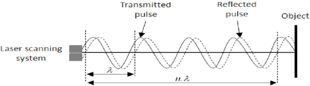
LIDAR enables remote sensing by measuring the Time Of Flight (TOF) of a laser pulse, and using this measurement to determine the distance of the object of which the laser is reflected. The distance of an object is calculated from the time it took the light beam to bounce and arrive back from and object. Since we know the speed of light, the total dis-tance traveled is simply given by the time multiplied by the speed of light.

𝑜𝑏𝑗𝑒𝑐𝑡 𝑑𝑖𝑠𝑡𝑎𝑛𝑐𝑒 =𝑡𝑖𝑚𝑒 𝑜𝑓 𝑓𝑙𝑖𝑔ℎ𝑡∗𝑠𝑝𝑒𝑒𝑑 𝑜𝑓 𝑙𝑖𝑔ℎ𝑡₂ (3.1)

The time interval of the reflected pulse can be also determined based on phase shift rang-ing method. In this method, the laser scannrang-ing system measures the phase difference be-tween the transmitted and reflected pulse.

𝑇 = 𝜆 (𝑛 + 𝜉/2𝜋) (3.2)

Where 𝑇 is the time interval, 𝜉 is the phase difference, 𝜆 is the wavelength of the pulse and n is the integer number which are measured using a digital pulse counting technique.

The range is estimated from the measured time interval using the distance time relation described in Equation 3.1. These equations are only an approximation; real-world systems adjust for error based on the intensity of the measured pulse returned, environmental and atmospheric conditions, distance to the scanned object, and many more circumstances which should be considered.

The method calculates the distance based on the phase of a returning pulse and in a coor-dinate system fixed to the laser scanner, not an absolute coorcoor-dinate system fixed to the earth. So the acquired data is defined with respect to the position and orientation of the scanner. As the acquisition platforms are mobile, the coordinate system is constantly changing and these measurements are difficult to use in their raw format; to simplify analysis of the LiDAR data, scan points are projected into a fixed coordinate system. For our data, this is a geodetic coordinate system, transforming each measurement into a tuple consisting of Latitude, Longitude, and Altitude (WGS84 coordinates).

This conversion is accomplished via a fusion process that correlates the raw range data with information from other sensors on the vehicle. Mobile laser scanning systems typi-cally rely on combination of Global Navigation Satellite Systems (GNSS) and Inertial Measurement Unit (IMU) technology for direct geo - referencing of the data. The primary instrument is a GNSS receiver, such as Global Positioning System (GPS) provide accu-rate positioning at low data frequency, typically 1-10 observations a second, when satel-lite visibility and constellation geometry is adequate. The GPS system accuracy can be compromised under a number of conditions, such as dense urban coverage, unfavorable GPS satellite configurations, and weather conditions. The acquisition vehicles also use an inertial measurement unit (IMU) in conjunction with wheel sensors to reduce drift in the GPS data. The IMU sensor measures micro-scale accelerations and changes in attitude at approximately 2 KHz. This data is used to interpolate how the system is moving in space (i.e., change in X, Y, Z and pitch, yaw, roll) between carrier-phase GPS measurements. Additionally, vehicles are equipped with a camera array that periodically obtains a color panorama of the surrounding environment. This panorama data can be correlated with the other sensory information.

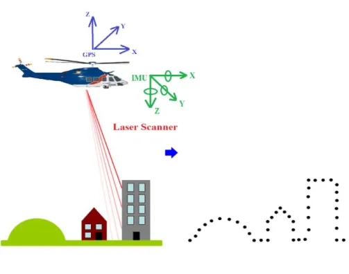
Different LiDAR vehicles have different operation principles, however following com-ponents are mostly common and have to work simultaneously for the generation of a precise digital surface model (see figure 1):

1. 360 panoramic camera: the imaging system along with laser scanning

2. Laser Range Finder (LRF): Measures the distance very accurately. It comprises the laser, transmission and receiving optics, the signal detector, the amplifier and the time counter.

3. Scanner: Deflects the laser beam across the path.

4. Global Positioning System (GPS): Determines the position and path of the vehi-cle using differential GPS positioning.

5. Inertial Measurement Unit (IMU): Measures acceleration and attitude changes and integrates them.

3.2 Types of LiDAR Systems

There are two types of urban LiDAR data acquisition in general: airborne and terrestrial. The urban 3D data can be scanned with airborne laser scanners. In this case the airborne laser scanner is generally handheld or mounted on a helicopter. Data acquisition for a terrestrial LiDAR system, on the other hand, is via a close-range terrestrial laser scanner mounted on a mobile robot or vehicle. There is a statistic terrestrial LiDAR which are typically used to capture features of interest in high detail. To capture large features such as buildings often requires taking multiple scans from different locations. Static scanners have the advantage of precision and affordability.

3.2.1 Airborne LiDAR

The Airborne laser scanning is an efficient system which can deliver very dense and ac-curate point clouds from the ground surface and the objects which are located on it. Providing high quality height information of the landscape by means of LIDAR systems opens up an extensive range of applications in different subjects in photogrammetry and remote sensing. The majority of change detection work in the context of Geographic In-formation System (GIS) is based on data obtained aerially. For urban applications, many research projects first make segmentation, and then attempt to monitor how segments change over time.

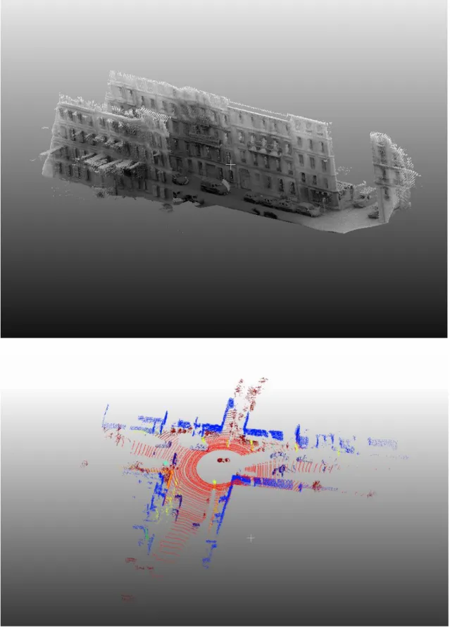
Figure 4.Example scanned and filtered MLS data from the NAVTEQ True system

3.2.2 Mobile Terrestrial LiDAR

The aerial and terrestrial Laser scanning systems which are used to acquire LiDAR data have different and specific usages in the computer vision applications. The data acquired from these systems differs in terms of its intrinsic accuracy and resolution for a variety of reasons but primarily due to the distance of the scanner to the target objects. In recent years, the use of terrestrial based moving vehicles has increased for the collection of high quality 3D data. Terrestrial laser scanning systems have utility towards accurate three-dimensional mapping of urban furniture (e.g. street signs, traffic lights, post boxes, traffic barriers, etc.), road details and vegetation. MLS provides rapid and dense capturing of 3D data for large street sections. The typical MTL vehicle is presented in figure 2 and an example of point cloud from MLS system is shown in figure 4. Terrestrial Laser Scanning (TLS) is a type of ground based LiDAR collecting which in it the LiDAR scanner and other sensors are stationary. In other word, MLS LiDAR is a type of TLS which the equipment are embedded on the top of a moving vehicle.

The ground based mobile LiDAR collection presents many opportunities, but it also pre-sents several challenges compared to aerial LiDAR mapping. A major advantage of ground based mobile LiDAR is that it allows a high-density, focused data collection along the targeted road path. Mobile collection enables true 3D data collection from multiple angles of access, except the roof view. In addition, multiple sensors such as panoramic cameras enable alignment and processing 2D and 3D word together. Another advantage of MLS is that it removes the need to close transportation corridors during data acquisi-tion, to put people in harm’s way, or to spend large sums of money on traditional survey-ing. For example, the vehicle can drive with traffic, the operators are within the vehicle, and the system can make tens of thousands of accurate measurements per second. The challenge is in using these measurements effectively.

The volume and structure of this data presents several challenges. The density of the 3D data collected by TLS scanners is due to the close proximity of the sensor to the targets. In addition, for large scale mapping, the collection vehicle may collect data spanning several hundred kilometers in a single day and for ideal data inspection close 3D viewing at the ground level and in the meter range is essential. Therefore, high techniques to save and display the datasets are needed. In addition, to generate usable geographic infor-mation based on unorganized point many challenges which could not be solved in some cases are listed below:

 Objects in the real street scene move while they are being scanned by MLS scan-ners, and the sensor itself is moving

 Sampling density varies with speed of vehicle acquisition system and surface ge-ometry

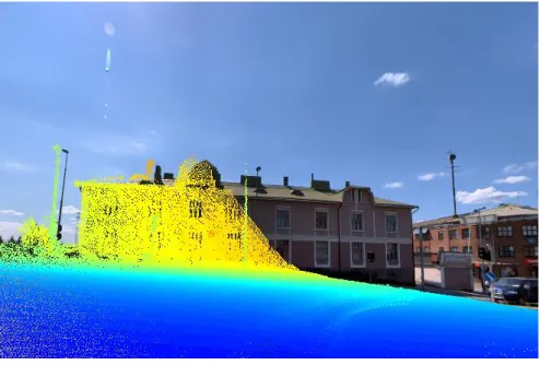
 Points rarely fall along object boundaries, it is so important especially in detecting thin objects such as pedestrians and sign symbols, see figure 5

 Foreground objects obstruct the scanners view of interest NAVTEQ True:

For the experiments, we made the algorithm automatically run through NAVTAQ true datasets provided by HERE. NAVTEQ mobile mapping system called NAVTEQ True, consists of best of sensors in three categories - positioning sensors, LiDAR sensors and imaging sensors. NAVTEQ was an American Chicago-based provider of geographic in-formation systems data and a major provider of base electronic navigable maps. The com-pany was acquired by Nokia in 2007/2008, and fully merged into Nokia in 2011 to form part of the HERE business unit. The sensors include a 360 panoramic camera for a nearly complete spherical view; multiple high resolution cameras for targeted view directions; a high density 360 rotating LiDAR system; and an inertial navigation system (IMU/GPS) for precise position and attitude tracking of the sensors. Information from all these sensors is synchronized to create an accurate and comprehensive data set that can be used for creation of accurate digital maps. The positioning system uses a high accuracy IMU, wheel sensors to measure the distance traveled and an L1/L2 GPS receiver. The LiDAR system has 64 lasers and rotates at 600 rpm covering a 360 degree field of view around the vehicle. The LiDAR system collects three dimensional point cloud at the rate of 1.3

Figure 5. Projection image and 3D LiDAR point cloud, presents the object

Figure 6. 3D point cloud in its noisy raw original format, Data collection vehicle “NAVTEQ True

3.3 Software used for programming and visualization

MATLAB and C++ were the two programming language used for this research. Matlab was mainly used due to its useful tools for image processing and visualization. Further-more Cloudcompare and Meshlab are used for the purpose of data visualization. Some Point cloud Library (PCL) tools used during our pipeline implementation. For details on this software library, please refer to [63]. Point Cloud Library is a stand-alone, large-scale, open project for 2D/3D image and point cloud processing. The library is freely available under a BSD license and the project is actively maintained through the collab-oration of many universities and the industry. The library also defines a widely used file format for storing point clouds. It is a simple format containing a header and the 3D in-formation, functions to read and write this format are available in the library.

ings from other LiDAR data points, where these two dominant classes often correspond to the majority of point clouds. Secondly, after removing these two classes, we use a pre-trained boosted decision tree classifier to label local feature descriptors extracted from remaining vertical objects in the scene. This work shows that the combination of unsu-pervised segmentation and suunsu-pervised classifiers provides a good trade-off between effi-ciency and accuracy. The output of classification phase is 3D labeled point cloud and each point is labeled with a predefined semantic classes such as building, tree, pedestrian and etc.

Given a labeled 3D point cloud and 2D cubic images with known viewing camera pose, the association module aims to establish correspondences between collections of labeled 3D points and groups of 2D image pixels. Every collection of 3D points is assumed to be sampled from a visible planar 3D object i.e. patch and corresponding 2D projections are confined within a homogenous region i.e. SuperPixels (SPs) of the image. The output of the 2D-3D alignment phase is 2D segmented image, in which every pixel is labeled based on 3D cues. In contrast to existing image-based scene parsing approaches, the proposed 3D LiDAR point cloud based approach is robust to varying imaging conditions such as lighting and urban structures.

The work flow which is used to achieve the objective of this research will be elaborated sequentially. As mentioned in chapter 1, the main process as well as the expected result will be discussed in section 4.1. After the proposed mythology workflow given, the de-tailed analysis for each process will be discussed in the following sections. The proposed method is evaluated both quantitatively and qualitatively and robust scene parsing results are reported in section 5.

4.1 Framework of the methodology

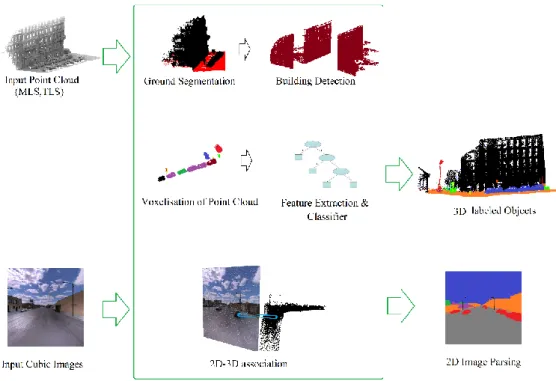
The framework of the proposed mythology is given in figure 7, in which 3D LiDAR point cloud and cubic images are the inputs of the processing pipeline and parsing results are presented as 3D labeled point cloud and 2D image segmented with different class labels e.g. Building, road, car and etc.

There are five main phases in the research: ground segmentation, building detection, voxelization, feature extraction-classification and 2D-3D association. Each phases will be discussed in detail in the following section.

Figure 7. Framework of proposed mythology

Figure 7 shows the overview of the proposed street scene object recognition pipeline, in which LiDAR point cloud and cubic images are the input of the processing pipeline and results are 3D PC and image segments assigned with different class labels. Because 3D cues are more robust compare to image features whole LiDAR data processing, segmen-tation, feature extraction and classification are done in 3D world.

At the outset, the proposed parsing pipeline finds ground points by fitting a ground plane to the given 3D point cloud of urban street scene. Then, non-ground point cloud are pro-jected to range images because they are convenient structure for visualization. Remaining data are processed subsequently to segment building facades. When this process is com-pleted, range images are projected to the 3D point cloud in order to make segmentation on other remained vertical objects. We use a connect component based algorithm to voxelization of data. The voxel based classification method consists of three steps, namely, a) voxelization of point cloud, b) merging of voxels into super-voxels and c) the supervised scene classification based on discriminative features extracted from super-voxels. Using a trained boosted decision tree classifier, each 3D feature vector is then designated with a semantic label such as tree, car, pedestrian etc. The offline training of the classifier is based on a set of 3D features, which are associated with manually labeled super-voxels in training point cloud. In the last phase 3D labeled PC are used to generate 2D image parsing result. Every images are segmented into superpixels to reduce compu-tational complexity and to maintain sharp class boundaries. Each superpixel in 2D image is associated with a class label based on labeled 3D patch.

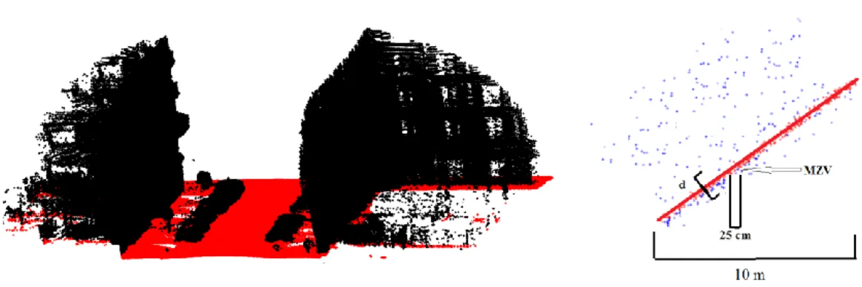
Figure 8. Ground Segmentation. Left image: Segmented ground and remained vertical objects point cloud are illustrated by red and black color respectively. Right figure: sketch map of fitting plane to one tile

4.2 Ground segmentation

The aim of the first step is to remove points belonging to the scene ground including road and sidewalks, and as a result, the original point cloud are divided into ground and vertical object point clouds (Figure 8). Given a 3D point cloud of an urban street scene, the pro-posed approach starts by finding ground points by fitting a ground plane to the scene. This is because the ground connects almost all other objects and we will use a connect component based algorithm to over‐segment the point clouds in the following step. The plane RANSAC fitting method is used to approximate ground section of the scene. The RANSAC algorithm was developed by Fischler et al. [64] and is used to provide a more robust fitting of a model to input data in the presence of data outliers. Unlike con-ventional model fitting techniques that use as much data as possible to obtain an initial solution, the RANSAC algorithm uses the smallest set of initial data required to fit a model and enlarges this set with compatible data. If there are enough compatible data, RANSAC can improve the estimation of the model, without having to deal with the data outliers. We will now describe the RANSAC algorithm in detail.

Suppose that we have n points in a dataset, X = x1, x2, … xn. A minimum required number

of m points are randomly selected, such that m ≤ n, to fit a least-square model M. The least-square model is fitted to the points based on minimizing the sum of square residuals which are the difference between the actual points and the fitted points. The model M is used to estimate data points in X (consensus points) which are within an error tolerance parameter, ε. If the number of consensus points is equal to or larger than a threshold, t, then a new least square model M* is fitted to these points. Otherwise, the whole process is repeated beginning with a random selection of m points. After some pre-set number of iterations, K, if the number of consensus points equal to or larger than t is not found, then

either the model fitted with the largest number of consensus points is accepted or the process is terminated unsuccessfully.

Given a 3D point cloud of an urban street scene, the scene point cloud is first divided into sets of 10m×10m regular, non-overlapping tiles along the horizontal x–y plane. Then the following ground plane fitting method is repeatedly applied to each tile. We assume that ground points are of relatively small z values as compared to points belonging to other objects such as buildings or trees (see Figure 8). The ground is not necessarily horizontal, yet we assume that there is a constant slope of the ground within each tile. Therefore, we first find the minimal-z-value (MZV) points within a multitude of 25cm×25cm grid cells at different locations. For each cell, neighboring points that are within a z-distance thresh-old from the MZV point are retained as candidate ground points. Subsequently, a RAN-SAC method is adopted to fit a plane to candidate ground points that are collected from all cells. The RANSAC algorithm uses three specified parameters as ε= 0.05 m, t = 7000 and K = 50. Finally, 3D points that are within certain distance (d in Figure 8) from the fitted plane are considered as ground points of each tile. The constant slope assumption made in this approach is valid for our data sets as demonstrated by experimental results in Section 5.

The approach is fully automatic and the change of two thresholds parameters do not lead to dramatic change in the results. On the other hand, the setting of grid cell size as 25cm×25cm maintains a good balance between accuracy and computational complexity.

4.3 Building segmentation

After segmenting out the ground points from the scene, we present an approach for auto-matic building surface detection. High volume of 3D data impose serious challenge to the extraction of building facades. Our method automatically extract building point cloud (e.g. doors, walls, facades, noisy scanned inner environment of building) based on two assumptions: a) building facades are the highest vertical structures in the street; and b) other non-building objects are located on the ground between two sides of street.

As can be seen in figure 9, our method projects 3D point clouds to range images because they are convenient structures to process data. Range images are generated by projecting 3D points to horizontal x–y plane. In this way, several points are projected on the same range image pixel. We count the number of points that falls into each pixel and assign this number as a pixel intensity value. In addition, we select and store the maximal height among all projected points on the same pixel as height value. We define range images by making threshold and binarization of I, where I pixel value is defined as equation 4.1

𝐼𝑖 =_{Max _𝑃}𝑃𝑖𝑛𝑡𝑒𝑛𝑠𝑖𝑡𝑦 𝑖𝑛𝑡𝑒𝑛𝑠𝑖𝑡𝑦 +

𝑃height

Figure 9. Building Segmentation

Where Ii is grayscale range image pixel value, Pintensity and Pheight are intensity and height

pixel value and Max_Pintensity and Max_Pheight represent the maximum intensity and height

value over the grayscale image. On the range image, an interpolation is required in order to fill holes caused by occlusions, missing scan lines and LiDAR back projection scatter. In the next step we use morphological operation (e.g. close and erode) to merge neigh-boring point and filling holes in the binary range images (see middle image in Figure9). The morphological interpolation does not create new regional maxima, furthermore it can fill holes of any size and no parameters are required. Then we extract contours to find boundaries of objects. In order to trace contours, Pavlidis contour-tracing algorithm [65] is proposed to identify each contour as a sequence of edge points. The resulting segments are checked on aspects such as size and diameters (height and width) to distinguish build-ing from other objects. More specifically, equation (4.2) defines the geodesic elongation E(X), introduced by Lantuejoul and Maisonneuve (1984), of an object X, where S(X) is the area and L(X) is the geodesic diameter.

E(π) =𝜋 𝐿_4𝑆(𝑋) 2 (𝑋) (4.2)

The compactness of the polygon shape based on equation (4.2) can be applied to distin-guish buildings from other objects such as trees. Considering the sizes and shape of build-ings, the extracted boundary will be eliminated if its size is less than a threshold. The proposed method takes advantage of priori knowledge about urban scene environment and assumes that there are not any important objects laid on the building facades. While this assumption appears to be oversimplified, the method actually performs quite well with urban scenes as demonstrated in the experimental results (see section 5).

The resolution of range image is the only projection parameter during this point cloud alignment that should be chosen carefully. If each pixel in the range image cover large area in 3D space too many points would be projected as one pixel and fine details would not be preserved. On the other hand, selecting large pixel size compared to real world resolution leads to connectivity problems which would no longer justify the use of range images. In our experiment, a pixel corresponds to a square of size .05 m2.

The 2D image scene is converted back to 3D by extruding it orthogonally to the point cloud space. The x–y pixels coordinate of the binary image labeled as building facades are preserved as x–y coordinate of 3D point cloud (with open z value) labeled as building, and not considered in the remainder of our approach. Other points (negligible amount compare to the size of whole PC) are labeled as non-building class and will be later be classified as other classes e.g. car, tree, pedestrian and etc.

4.4 Voxel based segmentation

After quick segmenting out the ground and building points from the scene, we use an inner street view based algorithm to cluster point clouds. Although top view range image analysis generates a very fast segmentation result, there are a number of limitation to utilize it for the small vertical object such as pedestrian and cars. These limitations are overcome by using inner view (lateral) or ground based system in which, unlike top view the 3D data processing is done more precisely and the point view processing is closer to objects which provides a more detailed sampling of the objects. However, this leads to both advantages and disadvantages when processing the data. The disadvantage of this method includes the demand for more processing power required to handle the increased volume of 3D data.

The 3D point clouds by themselves contain a limited amount of positional information and they do not illustrate color and texture properties of object. According to voxel based segmentation, points which are merely a consequence of a discrete sampling of 3D objects are merged into clusters voxels to represent enough discriminative features to label ob-jects. 3D features such as intensity, area and normal angle are extracted based on these voxels. The voxel based classification method consists of three steps, voxelization of point cloud, merging of voxels into super-voxels and the supervised classification based on discriminative features extracted from super-voxels. In the following two subchapters we present the concept and properties of voxels and supervoxels, and in the next chapters we present the way for extracting discriminative features from these 3D supervoxels.

Figure 10. Voxelization of Point Cloud. from top to down: top view row point cloud, voxelization result of objects point cloud after removing ground and building, s-voxeliza-tion approach of point cloud

4.4.1 Voxelization of Point Cloud

In the voxelization step, an unorganized point cloud p is partitioned into small parts, called voxel v. The middle image in figure 10 illustrates an example of voxelization re-sults, in which small vertical objects point cloud such as cars are broken into smaller partition. Different voxels are labelled with different colors. The aim of using voxeliza-tion is to reduce computavoxeliza-tion complexity by and to form a higher level representavoxeliza-tion of point cloud scene.

Following [66], a number of points is grouped together to form a variable size voxels. The criteria of including a new point pin into an existing voxel i is essentially determined

min( ‖𝑃_𝑖𝑚− 𝑃_𝑖𝑛‖₂) ≤ 𝑑_𝑡ℎ , 0 ≤ m, n ≤ N, m ≠ n (4.3) where pim is an existing 3D point in voxel, pin is a candidate point to merge to the voxel,

i is the cluster index, dth is the maximum distance between two point, and N is the

maxi-mum point number of a cluster. If the condition is met, the new point is added and the process repeats until no more point that satisfies the condition is found (see Algorithm 1). Equation (4.3) ensures that the distance between one point and its nearest neighbors be-longing to the same cluster is less than dth. Although the maximum voxel size is

prede-fined, the actual voxel sizes depend on the maximum number of points in the voxel (N) and minimum distance between the neighboring points.

The voxel example of one scene is presented in the middle image of Figure 10. Differ-ent voxels are labelled with differDiffer-ent colors.

4.4.2 Super Voxelization

For transformation of a voxel to super voxel we propose an algorithm to merge voxels via region growing with respect to the following properties of clusters:

 If the minimal geometrical distance, Dij, between two voxels is smaller than a

given threshold, where Dij is defined as equation (4.4):

𝐷𝑖𝑗 = min ( ‖𝑃𝑖𝑘− 𝑃𝑗𝑙‖₂) , k ∈ (1, m), l ∈ (1, n) (4.3) Where voxels vi and vj have m and n points respectively, and pik and pjl are the 3D

point belong to voxel vi and vj.

 If the angle between Normal vectors of two voxels is smaller than a threshold: In this work, normal vector is calculated using PCA (Principal Component Anal-ysis) [67]. The angle between two s-voxels is defined as angle between their nor-mal vectors as equation 4.5:

Repeat

Select a 3D point for Voxelization;

Find all neighboring points to be included in the voxel, with this condition that:

a point pin directly merge to voxel if its distance to any point pin the voxel

will not be farther away than a given distance (dth);

Until all 3D points are used in a voxel or the size of cluster is less than (N)

The advantage of this approach is that we can now use the reduced number of super voxels instead of using thousands of points in the data set, to obtain similar results for classifi-cation. The down image in figure 10 illustrates an example of s-voxelization results, in which different s-voxels are labelled with different colors.

4.5 Feature extraction and classification

For each s-voxel, seven main features are extracted to train the classifier. The seven fea-tures are geometrical shape, height above ground, horizontal distance to center line of street, density, intensity, normal angle and planarity. While the task of segmentation and classification traditionally relies on the color information alone, using such 3D infor-mation has some obvious advantages. Firstly it is invariant to lighting and/or texture var-iation; secondly it is invariant to camera pose and perspective change (view-independent fashion).

4.5.1 Feature extraction

In order to classify these s-voxels, we assume that the ground points have been segmented well. The object types are so distinctly different however these features as mentioned are sufficient to make a classification. Along with the above mentioned features, geometrical shape descriptors plays an important role in classifying objects. These shape-related fea-tures are computed based on the projected bounding box to x - y plane (ground).

Geometrical shape: Projected bounding box has effective features due to the invariant dimension of objects. We extract four feature based on the projected bonding box to rep-resent the geometry shape of objects.

 Area: the area of the bounding box is used for distinguishing large-scale objects and small ones, (see figure 11).

 Edge ratio: the ratio of the long edge and short edge.  Maximum edge: the maximum edge of bounding box.

 Covariance: is used to find relationships between points spreading along two larg-est edges.

Figure 11. Bounding box for tree

Height above ground: Given a collection of 3D points with known geographic coordi-nates, the median height of all points is considered as the height feature of the s-voxel. The height information is independent of camera pose and is calculated by measuring the distance between points and the road ground.

Horizontal distance to center line of street: Following [68], we compute the horizontal distance of the each s-voxel to the center line of street as second geographical feature. The street line is estimated by fitting a quadratic curve to the segmented ground.

Density: Some objects with porous structure such as fence and car with windows, have lower density of point cloud as compared to others such as trees and vegetation. There-fore, the number of 3D points in a s-voxel is used as a strong cue to distinguish different classes.

Intensity: following [69], LiDAR systems provide not only positioning information but also reflectance property, referred to as intensity, of laser scanned objects. This intensity feature is used in our system, in combination with other features, to classify 3D points. More specifically, the median intensity of points in each s-voxel is used to train the clas-sifier.

Normal angle: Following [70], we adopt a more accurate method to compute the surface normal by fitting a plane to the 3D points in each s-voxel. The surface normal is important properties of a geometric surface, and is frequently used to determine the orientation and general shape of objects. A surface normal is calculated using PCA (Principal Component Analysis). Given 3D point cloud data set D = x1, x2, x3, …,xn, the PCA surface normal

then associated with that particular voxel. In the experiments, we only estimate the normal direction for regions containing at least five 3D points. For diluted regions without suffi-cient points for normal estimation, we let this feature value to be 0.5.

Planarity: Patch planarity is defined as the average square distance of all 3D points from the best fitted plane computed by RANSAC algorithm. This feature is useful for distin-guishing planar objects with smooth surface like cars form non planar ones such as trees.

4.5.2 Classifier

The Boosted decision tree [71] has demonstrated superior classification accuracy and ro-bustness in many multi-class classification tasks. Acting as weaker learners, decision trees automatically select features that are relevant to the given classification problem. Given different weights of training samples, multiple trees are trained to minimize aver-age classification errors. Subsequently, boosting is done by logistic regression version of Adaboost to achieve higher accuracy with multiple trees combined together. Each deci-sion tree provides a partitioning of the data and outputs a confidence-weighted decideci-sion which is the class-conditional log-likelihood ratio for the current weighted distribution. The classifier training algorithm is given in Table 4.1. In the experiment the initial distri-bution is defined as proportional to the percentage density of whole point cloud spanned by each s-voxel, reflecting that correct classification of large s-voxel is more important than of small ones. When computing the log-likelihood ratio, we add a small constant (_2𝑚1 for m data samples) to the numerator and denominator which helps to prevent overfitting and to stabilize the learning process. We train separate classifiers to distinguish among the whole classes. These are each learned in a one vs. all fashion.

In our experiments, we boost 10 decision trees each of which has 6 leaf nodes. This pa-rameter setting is similar to those in [72], but with slightly more leaf nodes since we have more classes to label. The number of training samples depends on different experimental settings, which are elaborated in Section 5.

Table 4.1. BOOSTED DECISION TREES

For instance, to distinguish among the 10 defined classes, we train 10 classifiers that es-timate the probability of a s-voxel being car, pedestrian, tree or etc. These are then nor-malized to ensure that the estimated probabilities sum to one.

To train the classifiers, we need to assign ground truth to the automatically created S-voxel. If nearly all (at least 90%) of the 3D point within a s-voxel have the same ground truth label, the s-voxel is assigned that same label. Otherwise, the segment is labeled as “NoN” and we don’t use it for training phase. The classifier is then trained to distinguish among single-label segments. The classifiers use all of the listed features. Many of these cues can be quickly computed for the s-voxel, since the s-voxel cues provide sufficient statistics. The performance of the classification method is quite good, the result of the classier will be discussed in detail at chapter 5.

Input:

• D1...Dm: training data

• w1,1...w1,m: initial weights

• y1…ym ∈ {−1, 1}: labels

• nn: number of nodes per decision tree

• nt: number of weak learner decision trees

For t = 1...nt:

I. Learn nn-node decision tree Tt based on weighted distribution wt

II. Assign to each node Tt,k : ft,k= 1₂log

∑_{𝑖:𝑦𝑖=1 ,𝐷𝑖∈𝑇𝑡,𝑘} 𝑤𝑡,𝑖 ∑_{𝑖:𝑦𝑖=−1 ,𝐷𝑖∈𝑇𝑡,𝑘} 𝑤𝑡,𝑖

III. Update weights: wt+1,i =

1

1+exp(𝑦𝑖 ∑ 𝑓𝑡_{𝑡′ 𝑡′,𝑘𝑡′}) , with Kt’: Di ∈ Tt’,kt’ IV. Normalize weights so that ∑ 𝑤_{𝑖 t+1,i} = 1

Output:

• T1...Tnt : decision trees

Figure 12. From 3D world to image plane

4.6 2D-3D association

In this phase we propose a novel street scene image semantic parsing framework, which takes advantage of 3D labeled point clouds captured by a LiDAR laser scanner. Local 3D geometrical features extracted from s-voxel are classified by trained boosted decision trees and now they are used for labeling corresponding image segments. In contrast to existing image-based scene parsing approaches, the proposed point cloud based approach is robust to varying imaging conditions such as lighting and urban structures.

With the advancement of LiDAR sensors, GPS and IMU devices, large-scale, accurate and dense point cloud can be created and used for 2D scene parsing purpose. There has been a considerable amount of research in registering 2D images with 3D point clouds [73, 74]. Furthermore, there are methods designed for registering point cloud to image using LiDAR intensity [75].

The cubic images and 3D labeled LiDAR point cloud (output of chapter 4.5) are the inputs of the processing step and parsing results are image segments assigned with different class labels. The proposed parsing pipeline starts from aligning 3D LiDAR point cloud with 2D images. Input images are segmented into superpixels to reduce computational com-plexity and to maintain sharp class boundaries. Each superpixel in 2D image is associated with a collection of labeled LiDAR points, which is assumed to form a planar patch in 3D world. The detailed analysis for each process will be discussed in the following sub-sections.

4.6.1 Segmenting Images into Superpixels

Without any prior knowledge about how image pixels should be grouped into semantic regions, one commonly used data driven approach segments the input image into homo-geneous regions i.e. superpixels based on simple cues such as pixel colors and/or filter responses. The use of superpixels improves the computational efficiency and increases the chance to preserve sharp boundaries between different segments.

In our implementation, we adopt the geometric-flow based technique of Levinshtein [76] to segment images into superpixels with roughly the same size. Sharp image edges are also well preserved by this method. For input images with dimensionality of 2032×2032 pixels, we set the initial number of superpixels as 2500 for each image. See the image in figure 12 as the example of superpixel segmentation results.

4.6.2 LiDAR point cloud to Superpixel

Given a labeled 3D points cloud and one 2D image with known viewing camera pose, the association module described in this section aims to establish correspondences between collections of 3D points and groups of 2D image pixels. In particular, every collection of 3D points is assumed to be sampled from a visible planar 3D object i.e. patch and corre-sponding 2D projections are confined within a homogenous region i.e. superpixels of the image. While the 3D-2D projection between patches and superpixels is straightforward for known geometrical configurations, it still remains a challenging task to deal with out-lier 3D points in a computationally efficient manner. We first review how to project a 3D point on 2D image plane with known viewing camera pose, and then illustrate a method that associates a collection of 3D points with any given superpixel on 2D image.

Given a viewing camera pose i.e. position and orientation, represented, respectively, by T a 3×1 translation vector and R a 3×3 rotation matrix, and a 3D point M=[X,Y,Z]t, ex-pressed in a Euclidean world coordinate system, then the 2D image projection mp=[u,v]t

of the point M is given by equation 4.7.

𝑚̃𝑝 = k [ R | T ] 𝑀̃ = C 𝑀̃ (4.7) Where k is an upper triangular 3×3 matrix

𝐾 = [

𝑓𝑥 0 𝑥0

0 𝑓_𝑦 𝑦₀

0 0 1

] (4.8)

Where fx and fy are the focal length in the x and y directions respectively, x0 and y0 are

the offsets with respect to the image axes, and 𝑚̃_𝑝 = [𝑢, 𝑣, 1]𝑡and 𝑀̃ = [𝑥, 𝑦, 𝑧, 1]𝑡 are the homogeneous coordinates of mp and M.

are often measured in a geographic coordinate system (i.e. longitude, latitude, altitude), therefore, projecting a 3D LiDAR point on 2D image plane involves one more transfor-mation step, namely Geo-to-ECEF (equation 4.9).

𝑥 = (𝑁 + ℎ)𝑐𝑜𝑠𝜙 cos 𝜆 𝑦 = (𝑁 + ℎ)𝑐𝑜𝑠𝜙 sin 𝜆 (4.9)

Z= (N (1-e2_{) +h) sin 𝜙}

Where 𝜙, 𝜆 and h are latitude, longitude and height coordinate of 3D point. From WGS-84 the geodetic parameters equal to a= 6378137 and e2 =0.0067, where N is defined as

𝑁 = _√1−𝑒𝑎₂

𝑠𝑖𝑛2_𝜙 (4.10)

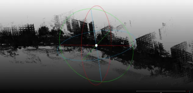
The relation between Geodetic (ellipsoidal) and ECEF coordinate system are shown in figure 13.

Figure 13. Coordinate conversion from Geodetic to ECEF

After this transformation, 3D point are transformed to local coordinate system NED (North=x East=y Down=z) by equation 4.7. Using these necessary transformation step and orthogonal projection, we are able to identify those 3D points that are projected within a specific SP.