Learning How To Recognize Faces In Heterogeneous Environments

(1)

2019

Acceptée sur proposition du jury

pour l’obtention du grade de Docteur ès Sciences par

Tiago DE FREITAS PEREIRA

Présentée le 14 juin 2019

Thèse N° 9366

Learning How To Recognize Faces In Heterogeneous Environments

Prof. P. Frossard, président du jury

Prof. H. Bourlard, Dr S. Marcel, directeurs de thèse Prof. M. Nixon, rapporteur

Prof. J. Fierrez, rapporteur Prof. J.-Ph. Thiran, rapporteur

à la Faculté des sciences et techniques de l’ingénieur Laboratoire de l’IDIAP

(2)

(3)

You’ll never walk alone — Richard Rodgers

(4)

(5)

Acknowledgements

This Ph.D. thesis is a result of years of work and it was supported by a lot of people.

First, I would like to thank Dr. Sébastien Marcel for opening the doors of Idiap and let me carry on my doctoral studies here and, most import, for his supervision. I am also grateful to my thesis director Prof. Hervé Bourlard, as well as the other members of my jury Prof. Mark Nixon, Prof. Julian Fierrez, Prof. Pascal Frossard and Prof. Jean-Philippe Thiran, for doing me the honor to supervise my oral exam.

Work at Idiap and EPFL is smooth thanks to the awesome administrative support from Nadine, Sylvie, Vanessa and Valérie, and the technical support of Bastien, Cédric, Frank, Louis-Marie, Norbert, Laurent and Vincent.

I also would like to thank my office mates that helped my a lot in the course of this thesis: Laurent, Ivana, Elie, Manuel, Pavel, Amir, Sulshil, Hannah, Vedrana, Guillaume, Olegs, Michael, Anjith, Zohreh, Pranay, Cijo, Gulcan, Pierre-Edouard, Nikos, Phil and David. Thanks to André for the great insights in the course of this journey as well as Ana and David for making my stay here in Switzerland very fun.

Many thanks to the guys from Samsung Research America for the opportunity to carry on my internship in the Mountain View campus and get to know the Silicon Valley. Specially, I would like to thank Bobi, Phillip, Sergi and Abhijit.

I would like to thank Prof. Sandra Aluísio from University of São Paulo and Prof. José Mario De Martino from University of Campinas for opening the doors of the university for me and let me start to think about research.

I’m also very thankful to the guys from CPqD for the friendship and the opportunity to start to investigate what machine learning is. I had a lot of help and everyone was very generous in key moments of my life. Specially, I would like to thank Norberto, Claudinei, Eliana, Henrique, Baldin, Flavio, Ricardo, Mario, Marcus, Dudu, Diego, Bruno, Vanessa, Amanda, Robson, Nagle, Paula and Stuchi.

Many thanks to my friends from Switzerland for the hospitality, friendship and generosity. Specially, I would like to thank Tiziana, Eduardo, Jolanta, Anne, Michael, Aurélie, Yoan and Audrey.

(6)

Thanks to the team from L’hôpital du Valais for fixing my legs twice in the course of this thesis. Special thanks to Jonatan, Yanik and Dr. Cédric Perez.

I also would like to thank my friend Laura for the patience and support in this final sprint. I’m also very thankful to my friends from Brazil that, apart from the distance, were very close in several instances of my life. Specially, I would like to thank Carolina, Bruno, Shimizu, Bruna, Bozoh, Camila, Marcus, Boulos, Moara, dona Lourdes, Scarton, Daniel and Larissa.

Special thanks must go to my parents Sueli and Tote and my brother Rodrigo and his girlfriend Thais for the love, support and to give me the freedom to pursue my dreams. I also would like to thank my grandfather Elias. His way of be is an example of strength and perseverance that I will take for life.

(7)

Abstract

Face recognition is a mature field in biometrics in which several systems have been proposed over the last three decades. Such systems are extremely reliable under controlled recording conditions and it has been deployed in the field in critical tasks, such as in border control and in less critical ones, such as to unlock mobile phones. However, the lack of cooperation from the subject and variations on the pose, occlusion and illumination are still open problems and significantly affect error rates. Another challenge that arose recently in face recognition research is the ability of matching faces from different image domains. Use cases encompass the matching between Visual Light images (VIS) with Near infra-red images (NIR), Visual Light images (VIS) with Thermograms or Depth maps. This match can occur even in situations where no real face exists, such as matching using sketches. This task is so called Hetero-geneous Face Recognition. The key difficulty in the comparison of faces in heteroHetero-geneous conditions is that images from the same subject may differ in appearance due to changes in image domain.

In this thesis we address this problem of Heterogeneous Face Recognition (HFR). Our con-tributions are four-fold. First, we analyze the applicability of crafted features used in face recognition in the HFR task. Second, still working with crafted features, we propose that the variability between two image domains can be suppressed with a linear shift in the Gaussian Mixture Model (GMM) mean subspace. That encompasses inter-session variability (ISV) modeling. Third, we propose that high level features of Deep Convolutional Neural Networks trained on Visual Light images are potentially domain independent and can be used to encode faces sensed in different image domains. Fourth, large-scale experiments are conducted on several HFR databases, covering various image domains showing competitive performances. Moreover, the implementation of all the proposed techniques are integrated into a collabo-rative open source software library called Bob that enforces fair evaluations and encourages reproducible research.

Keywords: Face Recognition, Heterogeneous Face Recognition, Reproducible Research, Do-main Adaptation, Gaussian Mixture Modeling, Deep Neural Networks

(8)

(9)

Résumé

La reconnaissance faciale est un domaine reconnu en biométrie, au sein duquel différents systèmes ont été proposés au cours des trois dernières décennies. De tels systèmes sont extrêmement fiables en conditions d’enregistrement contrôlées et ont été déployés sur le terrain, pour des tâches critiques telles que le contrôle aux frontières, et dans des cas moins critiques, par exemple pour déverrouiller des téléphones mobiles. Cependant, le manque de collaboration du sujet et les variations de la pose, l’occlusion et l’éclairage sont encore des problèmes ouverts qui affectent de manière significative les taux d’erreur. Un autre défi qui a surgi récemment au sein de la recherche en reconnaissance faciale est la capacité de faire correspondre des visages provenant de différents domaines d’image. Les cas d’utilisation englobent la correspondance entre les images Visual Light (VIS) avec les images infrarouge proches (NIR), les images Visual Light (VIS) avec les thermogrammes ou cartes de profon-deur (depth maps). Cette correspondance peut se produire même dans des situations où il n’existe aucun visage réel, telle que la correspondance avec des croquis médico-légaux. Cette tâche est appelée Reconnaissance Faciale Hétérogène (HFR). La principale difficulté dans la comparaison de visages en conditions hétérogènes est que les images d’un même sujet puissent avoir une apparence différente en raison des changements de domaine d’image. Dans cette thèse, nous abordons ce problème de Reconnaissance Faciale Hétérogène (HFR). Nos contributions sont au nombre de quatre. Premièrement, nous analysons l’applicabilité des caractéristiques conçues en reconnaissance faciale pour la tâche de HFR. Deuxièmement, toujours en travaillant avec ces caractéristiques, nous proposons que la variabilité entre deux domaines d’image puisse être supprimée par un décalage linéaire dans l’espace formé par le centres d’un Gaussian Mixture Model (GMM) mais également par la modélisation de la variabilité inter-session (ISV). Troisièmement, nous proposons que les caractéristiques de haut niveau d’un Deep Convolutional Neural Network entrainées sur des images Visual Light soient potentiellement indépendantes du domaine et puissent être utilisées pour encoder des visages détectés dans un domaine d’image différent. Quatrièmement, des expériences à grande échelle sont menées sur plusieurs bases de données HFR, couvrant différents do-maines d’image montrant des performances compétitives. De plus, toutes les techniques proposées sont intégrée dans une librairie logicielle collaborative opensource appelée Bob qui applique des évaluations non biasées et encourage une recherche reproductible.

Mots-clés: Reconnaissance faciale, Reconnaissance de visage, Reconnaissance Faciale Hété-rogène, Recherche Reproductible, Adaptation de domaine, Gaussian Mixture Modeling, Deep Neural Networks

(10)

(11)

List of Figures

1.1 Face recognition: Verification, Closed-set Identification and Open-set Identifica-tion tasks . . . 3 1.2 Examples of (a) low within-class variability (b) high within-class variability . . . 3 1.3 Example images from four different heterogeneous face recognition scenarious

(a) NIR (b) Thermal (c) Viewed sketch (d) Forensic sketch. . . 4 2.1 Basic structure of a Face Recognition System . . . 7 2.2 Principal Component Analysis (a) Definition of the new basis (b) The projection

inR1. . . 9 2.3 First two principal components using PCA vs FLD under four different sources

of illumination. Each color represents one of the 50 identities of the ARFACE database and each shape is one illumination condition (a) PCA face space (b) FLD face space . . . 11 2.4 Local Binary Pattern operator (a) Original image (b) LBP processed image . . . 12 2.5 Local Binary Pattern histograms . . . 12 2.6 Different ways to organize Gabor Jets. Extracted from [Günther, 2011, p.68] . . 13 2.7 Classical perceptron representation . . . 15 2.8 Classical MLP representation with three inputs and one hidden layer . . . 16 2.9 Classical MLP representation for two class classification task with three inputs

and one hidden layer . . . 17 2.10 Example of pooling a 2d input signal by patches of 2×2 . . . 18 2.11 Alexnet architecture [Krizhevsky et al., 2012] . . . 18 2.12 VGG19 architecture. Image extracted from[Simonyan and Zisserman, 2014] . . 19 2.13 One inception module composed by four parallel modules extracted from[Szegedy

et al., 2015] . . . 20 2.14 One residual connection extracted from[He et al., 2016] . . . 20 2.15 DCNN - Example of embedding extraction . . . 21 2.16 Realism of CUHK-CUFS database. Small details such as, the direction of the hair

and beard shape are the very similar . . . 22 2.17 Synthesized images generated with the method proposed by Wang and Tang

[2009]. Presented in the following order: Original photo, original sketch and synthesized sketch . . . 23

(16)

2.18 Different procedures to segment parts of the face experimented by Wang and

Tang [2009] and Peng et al. [2017] (images extracted from [Peng et al., 2017]) . . 23

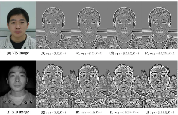
2.19 VIS and NIR images processed with Difference of Gaussians filter. Images taken from the CASIA NIR-VIS 2.0 database (see 2.3.1) . . . 24

2.20 Difference-of-Gaussians filter under different scales with VIS Images and NIR images. Images taken from the CASIA NIR-VIS 2.0 database (see 2.3.1) . . . 25

2.21 Image processing and feature extraction mechanism proposed by [Klare and Jain, 2013], the probe and gallery images are thermal and VIS images respectively. Note that for one image, six different combinations of pre-processing/features are extracted. . . 26

2.22 Application of LG-Face under different illumination conditions . . . 27

2.23 DCNN architecture proposed by [He et al., 2018] . . . 27

2.24 Wave lengths schematic. Extracted from Bourlai et al. [2010] . . . 28

2.25 Samples from CASIA NIR VIS 2.0 Database. Extracted from [Li et al., 2013]. . . . 29

2.26 Samples from NIVL Database. Extracted from [Bernhard et al., 2015]. . . 30

2.27 Samples from LDHF-DB Database collect at . (a) 1m (b) 60m (c) 100m (d) 150m. Extracted from [Kang et al., 2014] . . . 31

2.28 Example of images retrieved from the different streams of the camera. . . 32

2.29 Example of images acquired in each session. . . 32

2.30 The 16 annotated fiducial points. . . 33

2.31 Samples from CUHK CUFS Database. Extracted from [Bernhard et al., 2015]. . 34

2.32 Samples from CUHK CUFSF Database. Extracted from [Zhang et al., 2011]. . . . 36

2.33 Samples from Pola Thermal Database . . . 36

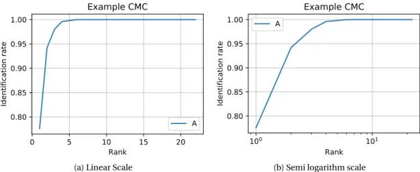
2.34 Cumulative Match Characteristics (CMC) curve under different scales in the x-axis of an arbitrary biometric system . . . 38

2.35 Example of DET curve of an arbitrary biometric system. It is possible to observe an FNMR@FMR=1%(dev) of≈5% in the Evaluation set . . . 39

3.1 Gabor Jets placed in different image modalities . . . 43

3.2 Max-Feature-Map (MFM) activate, whereh(x)=max(x1,x2) . . . 45

3.3 Difference-of-Gaussians filter crafted under different values forσ1,2and different kernel scalesK . . . 48

3.4 CUHK-CUFS Baselines - Average CMC curves (with error bars) . . . 50

3.5 CUHK-CUFSF Baselines - Average CMC curves (with error bars) . . . 52

3.6 Realism of CUHK-CUFS database . . . 53

3.7 VIS to NIR Baselines - Average CMC curves (with error bars) . . . 55

3.8 VIS and NIR images from NIVL dataset . . . 56

3.9 DET curves for the FARGO database verification experiments under the three illumination conditions MC (controlled), UD (dark) and UO (outdoor). The column on the left presents DET curves for the development set and the columns on the right presents DET curves for the evaluation set. . . 58

(17)

List of Figures

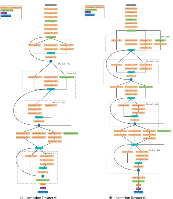
3.11 Inception Resnet architectures. Implementation inspired by Szegedy et al. [2017] 62 4.1 ISV Intuition (a) Estimation ofmandU (background model) (b) Enrollment

considering the session varibility using one sample . . . 69 4.2 ISV Intuition (a) Scoring using ISV (b) Scoring using MAP adaptation . . . 70 4.3 Feature extraction of the proposed approach . . . 72 4.4 CUFS - Average CMC curves (with error bars) using DCT coefficients and LBP

histograms varying the number of gaussians fromΘubm . . . 73

4.5 CUFS - Average CMC curves (with error bars) using DCT coefficients varying the rank ofU . . . 74 4.6 CUFSF - Average CMC curves (with error bars) using DCT coefficients and LBP

4.7 CASIA - Average CMC curves (with error bars) using DCT coefficients and LBP histograms varying the number of gaussians fromΘubm . . . 76

4.8 CASIA - Average CMC curves (with error bars) using DCT coefficients varying the rank ofU . . . 78 4.9 NIVL - Average CMC curves (with error bars) using DCT coefficients and LBP

4.10 FARGO - DET curves for verification experiments under the three illumination conditions MC (controlled), UD (dark) and UO (outdoor) trained with ISV. The column on the left presents DET curves using DCT coefficients as input and the column on the right presents DET curves using LBP histograms as a basis . . . 84 4.11 Thermal - Average CMC curves (with error bars) using DCT coefficients and LBP

histograms . . . 85 4.12 Pola Thermal - Average CMC curves (with error bars) using DCT coefficients and

LBP histograms . . . 87 5.1 Domain Specific Units - General Schematic . . . 92 5.2 Domain Specific Units learnt with Siamese Neural Networks given a pair of

samplesxs andxtfrom source and target domain respectively. (a) Forward pass

behaviour (b) Backward pass behaviour . . . 93 5.3 Domain Specific Units learnt with Triplet Neural Networks given a triplet of

samples: x_safromDs, andx_tpandx_tnfromDt. (a) Forward pass behaviour (b)

Backward pass behaviour . . . 95 5.4 CUFS - Average CMC curves (with error bars) for the adaptation of biases only . 99 5.5 Average rank one recognition rate vs number of parameters learnt . . . 100 5.6 CUHK-CUFS - Training loss forθt[1−6]using Siamese Networks. Check points at

every 100 steps. . . 101 5.7 CUFS - Average CMC curves (with error bars) for the adaptation of kernel and

biases . . . 102 5.8 CUFSF - Average CMC curves (with error bars) for the adaptation of biases only 104 5.9 CUFS - Average CMC curves (with error bars) for the adaptation of kernel and

(18)

5.10 CASIA - Average CMC curves (with error bars) for the adaptation of biases only 109 5.11 CASIA - Average CMC curves (with error bars) for the adaptation of biases and

kernels . . . 110 5.12 NIVL - Average CMC curves (with error bars) for the adaptation of biases only . 113 5.13 NIVL - Average CMC curves (with error bars) for the adaptation of kernel and

biases . . . 114 5.14 FARGO -Adaptingβonly- DET curves for verification experiments under the

three illumination conditions MC (controlled), UD (dark) and UO (outdoor) trained with Siamese Networks. The column on the left presents DET curves using Incep. Res. v1 as a basis and the column on the right presents DET curves using Incep. Res. v2 as a basis. . . 122 5.15 FARGO -AdaptingW +β- DET curves for verification experiments under the

three illumination conditions MC (controlled), UD (dark) and UO (outdoor) trained with Siamese Networks. The column on the left presents DET curves using Incep. Res. v1 as a basis and the column on the right presents DET curves using Incep. Res. v2 as a basis . . . 125 5.16 Thermal - Average CMC curves (with error bars) for the adaptation of biases . . 127 5.17 Thermal - Average CMC curves (with error bars) for the adaptation of kernel and

biases . . . 128 5.18 Pola Thermal - Average CMC curves (with error bars) for the adaptation of biases 131 5.19 Pola Thermal - Average CMC curves (with error bars) for the adaptation of kernel

and biases . . . 132 5.20 t-SNE scatter plots from the test set of the Thermal database before and after

DSU adaptation. Each color is one different identity and each shape is one of the two image modalities . . . 136 5.21 t-SNE scatter plots from the test set of the CUHK-CUFSF database before and

after DSU adaptation. Each color is one different identity and each shape is one of the two image modalities . . . 137 5.22 Fourier transform over the Incep. Res. v2 Conv2d_1a_3x3 convoluted images. (a)

and (d) corresponds to VIS images convoluted with feature detectors fromθs.

(b) and (e) corresponds to Thermal images convoluted with feature detectors fromθt before the DSU adaptation. (c) and (f ) corresponds to Thermal images

convoluted with feature detectors fromθt after the DSU adaptation. . . 138

B.1 Samples from the MSCeleb dataset . . . 148 C.1 Example images of the UCCS dataset1 . . . 151 C.2 Examples of pose, occlusion and blurriness variations of the UCCS dataset1 . . 152 C.3 Detection & Identification Rate curve published in 2nd Unconstrained Face

Detection and Open Set Recognition Challenge. The systems A4 for and A5 stands for the DSUθt[1−1]andθt[1−2]respectively. . . 153

(19)

List of Tables

2.1 Summary of the different protocols for heterogeneous face recognition: c stands

for controlled,dfor dark andofor outdoor. . . 33

2.2 Summary of all database characteristics . . . 37

3.1 The VGG16 architecture . . . 44

3.2 The Light CNN architecture . . . 45

3.3 VIS to Sketches - Average rank one recognition rate under different Face Recog-nition CNN systems. . . 51

3.4 VIS to NIR - Average rank one recognition rate under different Face Recognition systems . . . 54

3.5 LDHF average rank one recognition rates under different standoffs . . . 56

3.6 Fargo database - FNMR@FMR=1%(dev) taken from the development set . . . . 57

3.7 VIS to Thermograms - Average rank one recognition rate under different Face Recognition systems. . . 60

4.1 CUHK-CUFS - Average rank one recognition rate under different feature setups for ISV . . . 75

4.2 CUHK-CUFSF - Average rank one recognition rate under different feature setups for ISV . . . 77

4.3 CASIA - Average rank one recognition rate under different Face Recognition systems . . . 79

4.4 NIVL - Average rank one recognition rate under different Face Recognition systems 80 4.5 LDHF - average rank one recognition rates under different ISV setups . . . 81

4.6 Fargo database - FNMR@FMR=1%(dev) taken from the development under different ISV setups . . . 83

4.7 Thermal database - Average rank one recognition rate under different feature setups for ISV . . . 86

4.8 Pola Thermal database - Average rank one recognition rate under different fea-ture setups for ISV. . . 88

5.1 List of variables adapted for each one the tested architectures . . . 96 5.2 CUHK-CUFS - Average rank one recognition rate under different DSU training. 103 5.3 CUHK-CUFSF - Average rank one recognition rate under different DSU training. 107

(20)

5.4 CASIA - Average rank one recognition rate under different Face Recognition systems . . . 111 5.5 NIVL - Average rank one recognition rate under different Face Recognition systems115 5.6 LDHF - average rank one recognition rates under different stand-offsadapting

βonly . . . 118 5.7 LDHF - average rank one recognition rates under different stand-offsadapting

β+W . . . 120 5.8 Fargo database - FNMR@FMR=1%(dev) taken from the development set

adapt-ingβonly . . . 123 5.9 Fargo database - FNMR@FMR=1% adaptingW+β . . . 126 5.10 Thermal database - Average rank one recognition rate under different Face

Recognition systems. . . 130 5.11 Pola Thermal database - Average rank one recognition rate under different Face

Recognition systems. . . 134 5.12 Number of free parameters learnt for each base DCNN adapting eitherβorβ+W135 B.1 Mobio - HTER% using the mobio-male protocol . . . 149 B.2 LFW - TPIR% under different FMR thresholds . . . 149 B.3 LFW - TPIR% under different FMR thresholds . . . 149

(21)

1 Introduction

Biometrics is the field that addresses the task of identifying human beings by their physical and/or behavioral attributes [Ross et al., 2008]. Along the history, several biometric attributes have being researched, such as face, fingerprint, signature, voice, periocular, gait, DNA, palm veins, hand geometry, iris, ear, among others. Some of them are largely used in the industry, such as fingerprint, face, iris or palm veins and some are still work in progress in research laboratories, such as gait, ear or signature.

Face biometrics, in particular, has existed as a field of research for more than 40 years and its research has been active since the early 1990s. Such biometric trait has some advantages over others. First, it is natural among humans; we do face recognition on a daily basis. Second, it is non intrusive; interaction with special devices is not necessarily a requirement. Finally, it is potentially a good candidate for covert applications.

The current state-of-the-art in automated face recognition consists of systems that work well under relatively constrained conditions. Despite the research efforts over the last years, automated face recognition under unconstrained conditions, where variations on the pose, occlusion, illumination and collaboration of the subjects are not under control, is still a challenge. Among those challenges, one of the most challenging ones is the task of comparison of face images acquired between different image modalities (infrared images, forensic sketches, or thermograms). This field of research is calledHeterogeneous Face Recognitionand their use-cases can increase the robustness of face recognition systems in to more covert scenarios, such as recognition at a distance or at nighttime, or even in situations where no real face exists (forensic sketch recognition).

This thesis is a step towards the development of more robust systems for Heterogeneous Face Recognition (HFR).

(22)

1.1 Background and Motivations

Due to the maturity of face recognition research, numerous applications have appeared in the last few years. In the list below we highlight some of them:

1. Physical and Logical access control: Face recognition has been widely deployed in border control in the so callede-gates. During the 2008 summer olympic games in Beijing, a face recognition system was deployed into the entrance security checks for the opening and closing ceremonies [Jain and Li, 2011]. For several years Lenovo1allows users to unlock their laptops using face recognition technology. The same trend was followed by Apple that recently allowed users to unlock and authorize some transactions in their phones using face recognition2.

2. Surveillance and Law enforcement: The large amount of closed-circuit television (CCTV) systems deployed has led to a huge amount of information to be stored and processed. This is of particular interest in law enforcement, since face recognition technology can be employed to reduce the quantity of information to be processed manually, while criminal or terrorism investigations are performed. Several police departments around the world use software to compose sketches in eye witnesses cases, such as Evofit (https://evofit.co.uk/), Identikit (http://identikit.net/) and Faces (https://facialcomposites.com/) and the match of those composite sketches with large mugshot and legacy datasets raised the attention of the research community [Klare et al., 2011; Han et al., 2013].

3. Data Management and entertainment: Face identification has been widely used to automatically tag photos and/or video content. Companies such as Google, Microsoft, Facebook or Apple are already providing this feature in their image organizers and image viewer softwares to assist users in the task of organizing visual content and mitigate manual labor. Face identification is also applied in content personalization. For instance, game consoles such as XBox and PlayStation 4 allow users to log in to their online game platforms using face recognition.

The aforementioned applications can be reduced and formalized in three different tasks. (i) - The first one is calledverification, in which a person claims a particular identity, and the system has to verify this claim given a biometric trait as input. The cardinality of this task is 1:1. (ii) - The second task is calledclosed-set identification, in which the system has to identify a person from a setN possibilities in a gallery given a biometric trait as input. The cardinality of this task is 1:N. (iii) - The third and the last one is calledopen-set identification, in which the system has to identify a person from a setN possibilities if and only if the comparison score between the input biometric trait and the set ofN elements in the gallery is higher than

1_{https://www.lenovo.com}

(23)

1.1. Background and Motivations

a decision thresholdτ. The cardinality of this task is also 1:N. These distinctions are depicted in Figure 1.1. Claime d ide ntity Input biometric trait

Verific ation

Authe ntic ated Impostor

Input biometric trait

Close d-se t Identification

Identity 1 Identity 2 ... Identity N

Input biometric trait

Ope n-se t Identification

Identity 1 ... Identity N Unk now n

Figure 1.1 – Face recognition: Verification, Closed-set Identification and Open-set Identification tasks The ability to recognize faces is a natural action performed by humans and make us think that is an easy task to be generalized and statically programmed. In reality, its complexity is so high and with so many degrees of freedom that, so far, we were not able to define a generalized theory that is able to differentiate two random face images in any condition. For this class of tasks, a new field of knowledge emerged as a mix of Computer Science and Statistics called Machine Learning [Samuel, 1959]. Machine learning is a branch of artificial intelligence that considers that a particular task/phenomena can be learnt and generalized from a reduced set of its observations, without being explicitly programmed.

(a) (b)

Figure 1.2 – Examples of (a) low within-class variability (b) high within-class variability

As mentioned before, automatic face recognition is practically considered a solved problem for constrained scenarios where variations in illumination, pose, expression and/or collaboration of the subject are not “severe”. Variations in appearance on face images from the same person,

(24)

due to the mentioned factors, are called within-class variations. These variations can be as not as severe in the comparison between the images in Figure 1.2 (a) or can be very severe as in the comparison between the images in Figure 1.2 (b).

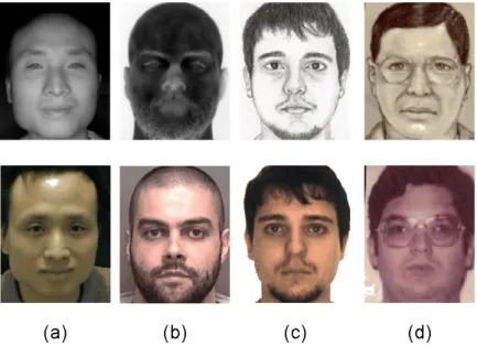
The task of HFR is considered challenging due to its high within-class variability between faces from the same subject but sensed in different image modalities. Example of these types of comparisons are shown in Figure 1.3.

Figure 1.3 – Example images from four different heterogeneous face recognition scenarious (a) NIR (b) Thermal (c) Viewed sketch (d) Forensic sketch.

1.2 Objectives and Contributions

The main objective of this thesis is to investigate methods to handle this high within-class variability between faces sensed in different image modalitites and, in consequence, increase recognition rates.

The major contributions of this thesis are as follows.

1. Domain Specific Units Framework (DSU)is proposed. We hypothesize that high level features of Deep Convolutional Neural Networks trained on visual spectra images are potentially domain independent and can be used to encode faces sensed in different image domains. A generic framework for Heterogeneous Face Recognition is proposed by adapting Deep Convolutional Neural Networks low level features and/or their biases only. The adaptation using Domain Specific Units allow the learning of shallow feature detectors specific for each new image domain. Furthermore, it handles its transforma-tion to a generic face space shared between all image domains.Related papers for this

(25)

1.3. Thesis Outline

contribution:[de Freitas Pereira et al., 2019] and http://vast.uccs.edu/Opensetface/. 2. Investigation of the face recognition strategies to the HFR task. We analyze and make

public available the effectiveness of some state-of-the-art face recognition systems in the academia and commercial of the shelf (COTS) trained with visual light images only in theH F Rtask.Related papers for this contribution:[de Freitas Pereira et al., 2019]. 3. HFR as Gaussian Mixture Model session variability problemis proposed. We

hypoth-esize that the task of HFR can be approached with a linear shift in the Gaussian Mixture Model (GMM) mean subspace. Such domain shifts can be estimated with inter-session variability (ISV) modeling, joint factor analysis (JFA) and total variability (TV) modeling. Related papers for this contribution: [de Freitas Pereira and Marcel, 2015] [de Fre-itas Pereira and Marcel, 2016] [Sequeira et al., 2017].

4. We successfullyapply the proposed approachesin several HFR databases covering six pairs of different image modalities and the results in terms of error rates are competitive with respect to the state of the art. Furthermore, this work is made reproducible in the following link3. Each one of the techniques applied in this thesis is part of the open source framework for signal processing and machine learning called Bob4following the reproducibility methodology defined in [Anjos et al., 2017]. In this methodology, it is emphasized that a reproducible research work should berepeatable, shareable, extensible, and stable.Related papers for this contribution:[Anjos et al., 2017].

1.3 Thesis Outline

This thesis is composed of 6 chapters.

In this chapter, the motivations, objectives and contributions of this work were briefly summa-rized.

Chapter 2 gives an overview of related work for the tasks of face and heterogeneous face recognition. In addition, this chapter introduces all the databases used in this work with its corresponding evaluation methodologies, which are used to compare the proposed systems in the experimentation chapters.

Chapter 3 presents how the state of the art face recognition systems developed in the academia and in the industry performs in the Heterogeneous Face Recognition task. Furthermore, a strategy base on Geodesic Flow Kernel using crafted features is introduced for HFR.

Chapter 4, the Gaussian Mixture Model framework for HFR is introduced. Consequently, the session variability modelling techniques that are built on top of this GMM are described for the HFR task. Moreover, experiments and analysis are presented.

3_{http://gitlab.idiap.ch/bob/bob.thesis.tiago} 4_{https://www.idiap.ch/software/bob/}

(26)

Chapter 5 introduces the Domain Specific Units (DSU) framework which is another technique to handle the HFR task. In this framework we hypothesize that high level features of Deep Convolutional Neural Networks trained on Visual Light images are potentially domain in-dependent and can be used to encode faces sensed in different image domains. Moreover, experiments and analysis are presented.

Chapter 6 concludes this thesis by providing a summary of the major contributions and findings. Potential directions for future work are also discussed.

(27)

2 Related Work

In machine learning, the task of Face Recognition is phrased as a classification problem under the big umbrella of supervised learning [Bishop, 2006, p.3]. More generally, the classification task can be phrased as an interpolation problem in high-dimensional space. Such task can be described as follows: Given two random variablesXandY, whereX∈Rd(high d-dimensional feature space) with marginal distributionP(X) and a discrete set of labelsY ∈Z, the classi-fication task consists in to find a modelΘwhere the probability ofP(Y|X,Θ) is maximized. For the face recognition task, the variablesXandY are placeholder terms for a face dataset X={x1,x2, ...,xn} and their corresponding set of labelsY ={y1,y2, ...,yn}.

Along the years, several different strategies were proposed to solve this classification prob-lem. Nevertheless, regardless the implementations, the approaches usually rely on three key components, which are depicted in Figure 2.1.

Capture Face Detection Feature extraction Feature Vector Classification Database F eature _Vector

Figure 2.1 – Basic structure of a Face Recognition System

The first component isFace Detection. This step has a major impact on the performance of the entire face recognition system. Given either a single image or a video as input, an ideal face detector should be able to identify and locate all present faces regardless of their position, scale, orientation, expression and illumination conditions[Jain and Li, 2011].

(28)

extractor should be able to extract important information of the face which are both: (i) -robustagainst any kind of noise, such as, illumination effects, occlusion, pose variations, image blurring, etc; (ii) - highdiscriminativecapability between face images from different identities. To rephrase this, an ideal feature extractor should be able to extract features that have low within-class variability and high between-class variability.

The third step isClassification, which is in charge of predict an identity given a feature vector. In this chapter describes with more detail the efforts made in the literature to approach the second and the third aforementioned items for both Face (Section 2.1) and Heterogeneous Face Recognition (Section 2.2). Emphasizing HFR, in Section 2.3 it is described the databases available to work on the problem. Finally, in Section 2.4 the evaluation methodologies used for this task is introduced.

2.1 Face Recognition

Raw face images are often represented as high dimensional array of pixels of size m-by-n. Hence, face images can be seen as a vector embedded in aRm×nspace. Due to well known significant statistical redundancies (correlations) that such images contains, it is common to represented them in lower dimension manifolds [Ruderman and Bialek, 1994]. In the last decades we have witnessed numerous scientific publications that explore this direction and applied algebraic, signal processing and statistical tools for extraction and analysis of the underlying manifold. In face analysis this manifold has a special name and it is calledface space[Jain and Li, 2011].

In this section it is briefly described in roughly chronological order the approaches designed along the years to build this face space.

2.1.1 EigenFaces

Turk and Pentland [1991] proposed the first feature-based automatic face recognition system in the beginning 1990s based on Principal Component Analysis. Principal Component Analy-sis (PCA) is a dimensionality reduction technique that uses an orthogonal transformation to convert a set of correlated variables into a set of values of linearly uncorrelated variables called principal components. This basis transformation is built in such a way that the vector direc-tion of the first principal component has the largest possible variance, the second principal component has the second largest possible variance and so on. This idea is illustrated in Figure 2.2 (a) where, inR2space, the new basis is defined and in Figure 2.2 (b) the first component of this new basis is preserved rather than a second and it’s used to do the projection inR1. In short, PCA tries to create a projection matrixΘwhere the L2 reconstruction (Equation 2.1) is minimized.

(29)

2.1. Face Recognition

x

1

x

2 (a)

x

1

x

2 (b)

Figure 2.2 – Principal Component Analysis (a) Definition of the new basis (b) The projection in

R1 ²(x)= ||x− k X i=0 (ΘT_ix)Θi|| (2.1)

There are several ways to achieve that. One of them is via the eigen decomposition of the co-variance matrix. Given a set of samplesX={x1,x2, ...,xn} wherex∈Rd, this can be calculated

following the steps below:

µ=1

n

n X

i=1

xiMean of the dataset (2.2a)

Σ= 1

n

n X

i=1

(xi−µ)(xi−µ)>Compute the covariance (2.2b)

Compute eigenvectorsU=[u1...ud] ofΣwhere (2.2c)

(Σ−ejI)uj=0, (2.2d)

whereejis the corresponding eigenvalues andj=1..d.

Another way to compute this face space is via singular value decomposition (SVD) ofX:

(30)

where the eigenvectors is given byUand the eigenvalues is given byd i ag(V).

The Eigenfaces pipeline can be explained as the following. Attraining time(offline), this face spaceΘis estimated given a face datasetX={x1,x2, ...,xn}∈Rd. Atenrollment time, given

one enrollment face imagexe∈Rd, its projection is computed asxe0 =ΘTxe. Atscoring time,

given one probe face imagexp∈Rdits projection is computed asxp0 =ΘTxp. To comparex0e

andx0pany distance measure can be used. Traditionally the L2 norm is employed, but other

metrics are very popular too, such as the Mahalanobis distance or the cosine similarity.

2.1.2 Fisher Linear Discriminant; “Fisherfaces”

The face spaceΘ trained via Principal Component Analysis, although it uncorrelates the image input space, does not approach the desired requirements of low within-class and high between-class variability. In unconstrained scenarios, part of the variability in the face appearance is due to severe variations in pose, illumination, expression, etc; and the PCA face space, possibly retains most of these variations. Belhumeur et al. [1996] propose to solve this problem with an application of Fisher’s linear discriminant (FLD)[Fisher, 1936]. Named as “Fisherfaces”, FLD selects aΘwhich maximizes the ratio:

ΘT_S bΘ ΘT_S wΘ (2.4) where Sb= m X i=0 Ni(xi−µ)(xi−µ)T (2.5)

is the between scatter matrix, and Sw= m X i=0 X x∈Xi (x−µi)(x−µi)T (2.6)

is the within scatter matrix.

This hypothesis explicitly finds a linear face spaceΘwhere the within-class variability is minimized while the between class variability is maximized. Furthermore, it also performs dimensionality reduction.

Figure 2.3 shows how the illumination effects are retained using PCA and how it is suppressed using FLD.

The Fisherfaces pipeline can be explained as the following. Attraining time(offline), this face spaceΘis estimated given a face datasetX={x1,x2, ...,xn}∈Rd. Atenrollment time, given

(31)

2.1. Face Recognition (a) front left right all (b) front left right all

Figure 2.3 – First two principal components using PCA vs FLD under four different sources of illumination. Each color represents one of the 50 identities of the ARFACE database and each shape is one illumination condition (a) PCA face space (b) FLD face space

Atscoring time, given one probe face imagexp∈Rdits projection is computed asx0p=ΘTxp.

To comparex_e0 andx0_pany distance measure can be used. Traditionally the L2 norm is used, but other metrics are very popular too, such as the Mahalanobis distance or the cosine similarity.

2.1.3 Local Binary Patterns histograms

The aforementioned sections presented strategies to model thisface spaceusing two different statistical hypotheses on top of the image space directly. Along the years, researchers also tried to craft their own set of features based on other assumptions.

The Local Binary Pattern (LBP) operator was originally designed for texture description [Ojala et al., 1996]. This operator is computed in a pixel level basis using aN×Nkernel, thresholding the surroundings of each pixel with the central pixel value and considering the result as a binary value. The decimal form of the LBP code is expressed as:

LB P(xc,yc)= N−1

X

i=0

f(Ii−Ic)2i, (2.7)

whereic corresponds to the gray intensity of the center pixel (xc,yc),N is the number of

sampling points,inis the gray intensity of the n-th surrounding pixel andf(x) is defined as

follows:

f(x)= (

0 ifx<0

(32)

Figure 2.4 shows how a face image in encoded in terms of their LBP decimals.

(a) (b)

Figure 2.4 – Local Binary Pattern operator (a) Original image (b) LBP processed image

Ahonen et al. [2004] proposed a face recognition system by histograming the LBP output. This method is non parametric, hence, there is nothing to be done attraining time. The technique first applies LBP encoding to each pixel of the face image and then divides the encoded face image into a set of windows. Histograms are then obtained from each region and concatenated to form a single feature vector. This is done atenrollmentandscoringtime. In Figure 2.5 it is possible to observe the application of this operator.

; Figure 2.5 – Local Binary Pattern histograms

Several metrics were developed to compare two LBP histograms. The most traditional one is the chi-square distance (χ2). Given two LBP histogramsXeandXp(for enrollment and for probing) theχ2is defined as follows:

χ2₍_Xe ,Xp)=X i,j wj (X_ie_,_j−X_ip_,_j)2 X_ie_,_j+X_ip_,_j . (2.9)

Furthermore, several classification strategies were proposed using LBPs as front end, such as Rodriguez and Marcel [2006a] with Gaussian Mixture Model and Pereira et al. [2012] with Support Vector Machines.

(33)

be found in [Pietikäinen et al., 2011].

2.1.4 Gabor Wavelets

There is a class of face recognition algorithms that rely on Gabor features. Such features are found to model the (retinal) image processing in the primary visual cortex of mamal brains [Daugman, 1985].

A Gabor wavelet [Würtz, 1995] defined as:

ψ~kj(~x)= ~k2_j σ2e − ~k2 j~x2 2σ2 h_ei~kÖj~x₋_e−σ 2 2 i (2.10)

is an image filter that consists of a planar complex wave ei~kTj~x _{that is confined by an}

en-veloping Gaussian and normalized to be mean free [Günther et al., 2017]. A Gabor wavelet is parametrized by the widthσof the Gaussian, its spatial orientationϕand the frequencyk [Günther et al., 2017]. Commonly, a family of 40 Gabor [Shen and Bai, 2006] wavelets are used to extract the features by discretizing the frequencies and orientations. Complex valued Gabor features are extracted by convoluting the input image with each one of the 40 Gabor wavelets. Traditionally, only the absolute parts of these complex valued features are taken into account [Günther et al., 2017].

(a) EBGM (b) Grid Graph

Figure 2.6 – Different ways to organize Gabor Jets. Extracted from [Günther, 2011, p.68] Based on Gabor wavelet responses, several algorithms were proposed. The most well-known example is the elastic bunch graph matching (EBGM) that was proposed in the late 1990s [Wiskott et al., 1997]. The EBGM algorithm for face recognition is non parametric; hence, there is nothing to be computed attraining time. Landmarks are detect and Gabor wavelet responses are computed in those detected regions of the face (see Figure 2.6a). All the Gabor wavelet responses computed in a particular region of the face are concatenated. The outcome of this concatenation is called Gabor Jet. Commonly the Gabor Jet is a result of the

(34)

concatena-tion of the absolute valuesaiand phasesφi. The Gabor Jets can also be computed in a grid

graph (see Figure 2.6b). Günther et al. [2017] indicated that grid graphs on average perform better than EBGM graphs. Atenrollmenttime, Gabor Jets are basically stored. Finally, at scoringtime, a comparison between stored and the probed Gabor Jet is carried out.

Given a stored Gabor jetJ and the probed Gabor jetJ0_{, with their corresponding absolute} valuesaand phasesφ, several metrics to compare them was proposed such as:

Scalar product: S(J,J0)=X i ai·a0_i (2.11) Camberra: S(J,J0)=X i ai−a0_i ai+a0_i (2.12) Absolute Phase: S(J,J0)=X i ai·a0_icos(φi−φ0_i) (2.13)

Zhang et al. [2005] proposed the combination between Gabor responses and LBPs. The technique called Local Gabor Binary Pattern Histogram Sequences (LGBPHS), applies Gabor wavelets at multiple scales and orientations to obtain several sub-images. These sub-images are then encoded using a standard MLBP operator and these local Gabor binary maps are then divided into non-overlapping regions. Then, a histogram is computed on each region. This approach is also non parametric; hence, nothing is done attrainingtime. Atenrollmenttime, such histogram are stored. Atscoringtime, a comparison between stored and the probed histograms is carried out using 2.9.

2.1.5 Deep Convolutional Neural Networks

Deep Convolutional Neural Networks have shown to be very powerful machine learning tool as they can be trained to learn complex non-linear mappings from high-dimensional data. But before its introduction, a more simple statistical model which is an elementary building block of those complex models shall be introduced: linear regression. Given a set of N input-output pairs X={(x1...xn)} andY ={(y1...yn)}, in linear regression, it is hypothesized that

exists a linear function mapping eachX ∈Rd toY ∈R. Such model in this case is a linear transformation of the inputs: f(x)=WÖ_X₊_β_{, where}_W _{is a 1}_×_d_{matrix and}_β_∈_R_{is a bias} term. Different values forW andβdefine different linear transformations and in general the goal is to find the parameters that minimizes some particular loss functionL. For instance,

(35)

such loss can be the mean square error defined as:L(W,β)= ||Y −(WÖ_X₊_β₎_||2

2. This is a

convex function and its global minima can be found using different methods, such as via closed-form. One of the most popular and scalable ones is the so called gradient descend which is depicted by the Algorithm 1.

Data:X,Y,i t,λ Result:W,β

W =random(dimension(X)) ; // Random initialization

β=0 ; // Usually initialized by 0 fori=0 to itdo forj=0 to size(X)do ∂L ∂W,β=y[j]−x[j]W+β; // Gradient W =W+λ_∂∂L_W; β=β+λ∂_∂βL; end end

Algorithm 1:Gradient descent training, whereXis am×dmatrix,Y is am×1 matrix,i tis the number of iterations of the algorithm andλis the learning rate

In most of the cases, specially in real world scenario, the relation betweenXandY is not linear and a non-linear basis functiong(x) that mapsXtoY has to be defined [Bishop, 2006, p.137]. Hence, the same linear regression can be performed between the pairX ={(g(x1)...g(xn)}

andY ={(y1...yn)}. These basis functions can be polynomials, logistic functions, ReLU1, etc.

This basic building block is often called Perceptron [Haykin, 2009, p.48] and its graphical representation is depicted in Figure 2.7.

Σ

g

+1

x

1

x

2

x

3

x

n

β

w

₁

w

2

w

3

w

n

g

_n

P

i=1

w

i

x

i

+

β

..

.

Figure 2.7 – Classical perceptron representation

The foundation of deep neural networks can be defined by a set those perceptrons stacked “vertically”, makingW an×dmatrix. For historical reasons, thisnis coined the number of

(36)

neurons. Furthermore, those perceptrons can also be stacked “horizontally”, hence, the non-linear outputs froml1=g(W₁ÖX+β1) can be provided as input to another set of non-linear

operations (called hidden layer)l2=g(W₂Öl1+β2) and finally thisl2can be forwarded to our

regressed outputo=g(W₃Öl2+β3). In this example,W1,W2andW3 isn1×d,n2×n1and

n2×1 matrices respectively. This mechanism of stacking those perceptrons is a very powerful

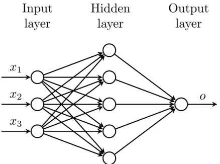
tool to solve very complex non-linear mappings and it is called Multi-Layer Perceptron (MLP) [Haykin, 2009, p.122]. Its classical graphic representation is depicted in Figure 2.8. The process

x

₁

x

₂

x

3 Input

layer

Hidden

layer

Output

layer

o

Figure 2.8 – Classical MLP representation with three inputs and one hidden layer

to learn all the possible values forW1,W2andW3for thisnon-convex functionis similar to

the one defined for linear regression. The gradient of a particular loss (e.g mean square error) with respect to eachW[1..3]andβ[1..3](_∂_W[1..3]∂L_,_β_[1..3]) has to be propagated to allW[1..3]andβ[1..3].

This is carried out by an algorithm called Back Propagation [Haykin, 2009, p.153].

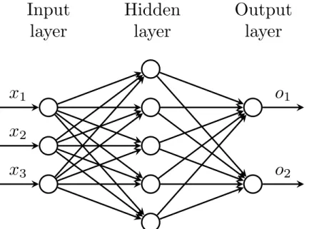
MLPs can also be used for classification. One way to approach such task is by adding as much as output peceptrons as the number of classes and makeY ∈Zc2, wherecis the number of

classes. Figure 2.9 presents an example of MLP for a two class problem.

For image classification, the selection of features (number of layers and number of neurons) for training a MLP is often empirical and data dependent. A possible solution to approach this issue would be to use directly the raw data and let the MLP training algorithm (Back Propagation) find the best feature extractors by adjustingW[1..n]andβ[1..n]. The problem with

this approach is that the dimensionality of the input data is often high (specially for image recognition), hence the number of free parameters (number of connections) is large, since each hidden unit is fully connected. Depending of the amount of data available for training, the neural network tends to overfit.

(37)

x

₁

x

2 x

3 Input

layer

Hidden

layer

Output

layer

o

₁

o

2

Figure 2.9 – Classical MLP representation for two class classification task with three inputs and one hidden layer

A Convolutional Neural Network (CNN) [LeCun et al., 1998] is an approach that tries to alleviate the aforementioned problem. Base perceptrons are replaced by alocallinear transformation called convolution that is discretely defined for 1d signals as:

w∗X= i=d X i=k/2 j=k/2 X j=−k/2 w[j]X[i−j], (2.14)

wherewis the convolutional operator also called kernel or filter of dimensionkandX is a 1d signal of dimensiond. This transformation is highly used in image processing since it preserves spatial information of an input image. The same non-linearity hypothesis can be hypothesized for this operation, hence, non-linear convolutions can be defined asg(w∗X). Furthermore, bias terms can be added to this operationg(w∗X)+β. These local linear transformations introduces a weight sharing in the neural networks that reduces drastically the number of free parameters that needs to be learnt, reducing the capacity of the network and improving its generalization capability. In Deep Convolutional Neural Networks, the convolutions are often followed by pooling layers. The purpose of such operation is to locally sub-sample the input signal by some statistical function. Figure 2.10 presents an example of pooling. In most practical cases in image recognition, the operatormaxis used and such operation is called MaxPooling. Such operations can be stacked as in the MLP and the process of learningwis the same as for MLPs (via Back Propagation).

The success of Deep Convolutional Neural Networks (DCNN) in computer vision research, the availability of several frameworks to instrument such networks and the possibility to work

(38)

Figure 2.10 – Example of pooling a 2d input signal by patches of 2×2

with massive amounts of labeled data (CASIA WebFace [Yi et al., 2014], MS-Celeb [Guo et al., 2016] and Megaface [Kemelmacher-Shlizerman et al., 2016]) made face recognition error rates decrease steadily.

Despite the lack of deep understanding on why such neural networks work well and have good generalization capabilities in several different pattern recognition tasks [Mallat, 2016], practical heuristics were developed in the last five/six years to regularize the training and they are responsible for its success in practice. In the next subsections we would like to highlight some that, in our experience, have direct impact in decreasing face recognition error rates.

Alexnet

Krizhevsky et al. [2012] released in 2012 the AlexNet DCNN. Such work put together seminal elements that are standard until today in any pattern recognition task that relies on DCNN, including face recognition. Its architecture is depicted in Figure 2.11.

; Figure 2.11 – Alexnet architecture [Krizhevsky et al., 2012]

Three seminal contributions worth mentioning in this work.First, it is about the depth of the DCNN. This network scale up the insights from LeNet[LeCun et al., 1998] and implemented a much deeper neural network composed by five convolutional layers and three fully connected layers. It was also roughly demonstrated that, in the case of object detection, depth matters. Thesecondcontribution was the usage of ReLU as activation function. In their work, the training was 6 times faster than thet anhfunction. Thethirdcontribution was the usage of dropout [Hinton et al., 2012] as one of the regularization strategies. They idea of dropout is to

(39)

Figure 2.12 – VGG19 architecture. Image extracted from[Simonyan and Zisserman, 2014]

randomly drop connections during the training stage. This can be seen as an approximation of bagging [Bishop, 2006, p.653].

VGG networks

The VGG networks [Simonyan and Zisserman, 2014] were the first to use small kernels in each convolutional layer (3×3) and push forward even more the limits of depth in deep neural networks.

Its main contribution was the usage of small convolutional kernels chained in a long sequence of convolutions (even longer than Alexnet). Followed by sub-samplings (pooling), this archi-tecture was able to detect image symmetries in larger areas of image that was thought possible only via larger kernels (5×5, 9×9 or 11×11) like in Alexnet or LeNet.

Figure 2.12 presents the schematic of one of the proposed VGG architectures.

Batch normalization

Introduced by Ioffe and Szegedy [2015], batch normalization consists in shifting (usually zero-mean) and scaling (normally one standard deviation) the output signal of each layer for each mini-batch.

(40)

Making this normalization part of the architecture allows the DCNN practitioners to be more “aggressive” with the learning rates and speeding up the convergence with larger architectures.

Inception modules

Szegedy et al. [2015] introduced the Inception modules. Those modules are composed by parallel combination of different convolutional kernels (1×1, 3×3, and 5×5 normally) as can be seen in Figure 2.13. This contribution allowed a dramatic reduction of free parameters to be learnt, increasing the recognition accuracies and generalization for several computer vision tasks.

Figure 2.13 – One inception module composed by four parallel modules extracted from[Szegedy et al., 2015]

Residual Connections

As mentioned in the last subsections, practical evidences in several areas of computer vision have shown that depth of a DCNN seems to be a crucial factor in terms for accurate learning. One of the main obstacles to explore depth in DCNNs is the well known gradient vanishing/-exploding [Glorot and Bengio, 2010] problem. He et al. [2016] approached this issue bypassing the output of one intermediate layer and concatenating as the input of one of the layers ahead (two or three layers) as we can see in Figure 2.14. Such approach allowed the training of CNNs larger than 1000 layers[He et al., 2016].

A common way to approach the FR task using DCNNs is to, attraining time, train it for a particular face dataset (n-class classification task). Then, it is hypothesized the feature detectors learnt for this particular classification task are generic and discriminative enough to be applied to other set of identities unseen by this training procedure. This can be carried out by taking the trained the DCNN and “drop” its outputs and make one of the hidden layers as the new output. Hence, this output can be used as a feature and be directly compared using an arbitrary metric, such as L2 norm, cosine similarity, Mahalanobis, etc. This feature is often calledembedding. Figure 2.15 presents a simple example on how this embedding generator

(41)

2.2. Heterogeneous Face Recognition

Figure 2.14 – One residual connection extracted from[He et al., 2016]

is created by dropping the classification output of DCNN.

2.2 Heterogeneous Face Recognition

In the beginning of this chapter a formalization of supervised learning was presented. We adapted the aforementioned formalization for the task of Heterogeneous Face Recognition and it is defined as the following. Let’s assume now that we have two domainsDs={Xs,P(Xs)} andDt={Xt,P(Xt)} called respectivelysource domainandtarget domainwith both sharing the same set of labelsY. Hence, the goal of Heterogeneous Face Recognition task is to find a

Θ, whereP(Y|Xs,Θ)=P(Y|Xt,Θ).

Several assumptions to modelΘwere proposed during the last years and we can organize them in three main categories, whose details are described in the following three subsections.

2.2.1 Synthesis methods

In these methods a synthetic version ofDsis generated fromDt. Once a synthetic version fromDtis generated, the matching can be done with regular face recognition approaches. In [Wang and Tang, 2009], the authors proposed a patch based synthesis method that syn-thesizes VIS images to sketches. Thereafter, synthesized sketches are feed into regular face recognition systems, such as Eigenfaces, Fisherfaces, dual spaceLD A. At training time, a Markov Random Field generative model, pairing patch nodes (pixel level) from source and target domains, is build in such a way that the probability of a set patches from the source domain given one patch from the target domain is maximized. Although there is no source code officially available for this work, a matlab implementation can be found in2. This al-gorithm provides very appealing reconstructions using the images from the CUHK-CUFS (see Section 2.3.2), where the sketches are very reliable with respect to their corresponding

(42)

x1 x2 x3 Input layer 1st Hidden layer 2nd Hidden layer Output layer o1 o2

(a) DCNN used at training time for a two class classification prob-lem x1 x2 x3 Input layer 1st Hidden layer Embedding e1 e2 e3

(b) DCNN used at enrollment and scoring time where the outputs are “dropped”

Figure 2.15 – DCNN - Example of embedding extraction

photographs. Even minimum details of shape and direction of the hair are preserved as we can observe in Figure 2.16. However, using less reliable hand drawn sketches databases, such as the CUHK-CUFSF (see Section 2.3.2) or other image modalities the reconstructions are very poor as we can see in Figure 2.17.

A slightly modification of the aforementioned approach was presented in [Peng et al., 2017]. Differently from [Wang and Tang, 2009], the authors replaced the patches by superpixels [Achanta et al., 2012] as we can observe in the Figure 2.18. An average rank one recognition rate of 99% and 72% was reported in CUHK-CUFS and CUHK-CUFSF databases respectively. Focusing in thermal images, Zhang et al. [2017] proposed a method based on Generative Adversarial Networks (GANs) in order to generate thermogram images from visual spectra images for further identification using the Pola Thermal dataset [Hu et al., 2016] (see Section 2.3.3). The identification is carried out using the Visual Geometry Group (VGG) network embeddings that are freely available3. Such synthesized images are feed into this DCNN and

(43)

2.2. Heterogeneous Face Recognition

Figure 2.16 – Realism of CUHK-CUFS database. Small details such as, the direction of the hair and beard shape are the very similar

(a) Example from CUHK-CUFS database (b) Example from CUHK-CUFSF database

Figure 2.17 – Synthesized images generated with the method proposed by Wang and Tang [2009]. Presented in the following order: Original photo, original sketch and synthesized sketch

compared. Using those embeddings, the authors published an Equal Error Rate (EER) of 25.17% using the ThermalPolarized procotols and an EER of 27.34% using the VIS-to-Thermal

Similarly, Zhang et al. [2018] also proposed a strategy based on GANs for the exact same task (VIS-to-Thermal). With slightly changes in the loss they presented a rank one recognition rate of 19.9% using the private dataset that covers the VIS-to-Thermal problem (with 29 pairs of images to train the GAN from scratch).

2.2.2 Crafted features-based methods

In these methods raw face images from both domains (DsandDt) are encoded with descrip-tors that are invariant between them.

Liao et al. [2009] proposed a very simple method for the task of VIS to NIR recognition, where both modalities are normalized using difference of gaussian filter as we can see in Figure 2.19. As feature descriptor, MutiScale Local Binary Patterns (MLBP)[Pietikäinen et al., 2011] (with

(44)

(a) Patch segmentation (b) Super pixels segmen-tation

Figure 2.18 – Different procedures to segment parts of the face experimented by Wang and Tang [2009] and Peng et al. [2017] (images extracted from [Peng et al., 2017])

(a) RGB image (VIS) (b) RGB image filtered (c) NIR image (d) NIR image filtered

Figure 2.19 – VIS and NIR images processed with Difference of Gaussians filter. Images taken from the CASIA NIR-VIS 2.0 database (see 2.3.1)

different radii) is used. Pairs of images VIS and NIR, processed with MLBP histograms, are used to trainF LDsystem (see Section 2.1). A verification rate of 67.5% was reported under a false acceptance rate of 0.1% on the CASIA-HFB [Liao et al., 2009] database.

Liu et al. [2012] hypothesized that independent features between VIS and NIR are embedded in a particular range of frequency bands. To approach that the authors searched a particular range of scales of MultiScale Difference-of-Gaussian filter. This search can be seen in Figure 2.20. The authors used two different types of feature descriptor on top of this multiscaled processed images. The first one is the Histogram of Oriented Gradients (HOG) and the Scale-invariant feature (SIFT) descriptor is extracted. The Gentle Boost is used as a classifier [Bishop, 2006, p.657]. A rank one recognition rate of 98.51% was reported in the CASIA HFB database. In a similar direction, Klare and Jain [2013] proposed an approach where face images from both domains are normalized using three different image processing filters (Difference-of-Gaussians, Center-Surround Divisive Normalization [Meyers and Wolf, 2008] and Gaussian Filter). Afterwards, two different feature local descriptors are extracted from patches of the

Learning How To Recognize Faces In Heterogeneous Environments

Tiago DE FREITAS PEREIRA

Thèse N° 9366

Learning How To Recognize Faces In Heterogeneous Environments

Acknowledgements

Abstract

Résumé

Contents

List of Figures

List of Tables

1

Introduction

1.1 Background and Motivations

Verific ation

1.2 Objectives and Contributions

1.3 Thesis Outline

2

Related Work

2.1 Face Recognition

x

x

x

x

Σ

g

+1

x

x

x

x

β

w

w

w

w

g

P

w

x

+

β

..

.

x

1

x

2

x

3

Input

layer

Hidden

layer

Output

layer

o

x

1

x

2

x

3

Input

layer

Hidden

layer

Output

layer

o

1

o

2

2.2 Heterogeneous Face Recognition

₁

₂

₁

₁