Munich Personal RePEc Archive
Bayesian Fuzzy Clustering with Robust
Weighted Distance for Multiple ARIMA
and Multivariate Time-Series
Pacifico, Antonio
LUISS Guido Carli University, CEFOP-LUISS, LUISS Guido Carlo
University
2020
Online at
https://mpra.ub.uni-muenchen.de/104379/
Bayesian Fuzzy Clustering with Robust Weighted Distance
for Multiple ARIMA and Multivariate Time-Series
Antonio Pacifico
*Abstract
The paper suggests and develops a computational approach to improve hierarchical fuzzy clustering time-series analysis when accounting for high dimensional and noise problems in dynamic data. A Robust Weighted Distance measure between pairs of sets of Auto-Regressive Integrated Moving Average models is used. It isr obust because Bayesian Model Selection methodology is performed with a set of conjugate informative priors in order to discover the most probable set of clusters capturing different dynamics and interconnections among time-varying data, andwei g ht edbecause each time-series is ’adjusted’ by own Posterior Model Size distribution in order to group dynamic data objects into ’ad hoc’ homogenous clusters. Monte Carlo methods are used to compute exact posterior probabilities for each cluster cho-sen and thus avoid the problem of increasing the overall probability of errors that plagues classical statistical methods based on significance tests. Empirical and simulated examples describe the functioning and the performance of the procedure. Discussions with related works and possible extensions of the methodology to jointly deal with endogeneity issues and misspecified dynamics in high dimensional multicountry setups are also displayed.
JEL classification: A1; C01; E02; H3; N01; O4
Keywords: Distance Measures; Fuzzy Clustering; ARIMA Time-Series; Bayesian Model Se-lection; MCMC Integrations.
*Corresponding author: Antonio Pacifico, Postdoc inApplied Statistics & Econometrics, LUISS Guido Carli University, CEFOP-LUISS (Rome), CSS Scientific Institute (Tuscany). Email: [email protected] or [email protected]. ORCID:https://orcid.org/0000-0003-0163-4956
1 Introduction
With increasing power of data storages and processors, several applications have found the chance
to store and keep data for a long time. Thus, data in many applications have been stored in the
form of time-series data. Generally, a time-series is classified as dynamic data because its feature
values change as a function of time, which means that the values of each point of a time-series are one or more observations that are made chronologically (see, e.g., Keogh and Kasetty (2003)
and Rani and Sikka (2012)). The intrinsic nature of a time-series is usually that the observations
are dependent or correlated. The Auto-Regressive Integrated Moving Average (ARIMA) processes
are a very general class of parametric models useful for describing dynamic data and their
cor-relations. This amount of time-series data has provided the opportunity of analysing time-series
for many researchers in data mining communities in the last decades. Consequently, many
re-searches and projects relevant to analyze time-series have been performed in various areas for
different purposes such as: subsequence matching; clustering; identifying patterns; trend analy-sis; and forecasting. It has carried the need to develop many on-going research projects aimed to
improve the existing techniques (see, for instance, Zakaria et al. (2012) and Rakthanmanon et al.
(2012)).
Time-series data are of interest because of its pervasiveness in various areas such as: business;
finance; economic; health care; and government. Given a set of unlabeled time series, it is
of-ten desirable to determine groups (or clusters) of similar time-series. These time-series could be
monitoring data collected during different periods from a particular process or from more than
one process. Generally, clusters are formed by grouping objects that have maximum similarity
with other objects within the group, and minimum similarity with objects in other groups. It is a useful approach for exploratory data analysis as it identifies structures in an unlabelled dataset
by objectively organizing data into similar groups. The goal of clustering is to identify structure
in an unlabeled data set by grouping data objects into a tree of homogeneous clusters, where the
within-group-object similarity is minimize and the between-group-object dissimilarity is
max-imized. Nevertheless, works devoting to the cluster analysis of time-series are relatively scant
compared with those focusing on static data. In addition, a pure hierarchical clustering method
suffers from its inability to perform adjustment once a merge or split decision has been executed.
Thus, for improving the clustering quality of hierarchical methods, there is a trend of increased activity to integrate hierarchical clustering with other clustering techniques.
My approach and empirical application aim to give a valid contribution to such topics. More
precisely, when dealing with time-series, a suitable measure to evaluate the similarities and
dis-similarities within the data becomes necessary and subsequently it exhibits a significant impact
on the results of clustering. This selection should be based upon the nature of time-series and the
application itself. In this context, hierarchical fuzzy clustering tends to hold a relevant
compet-itive position. It is a data mining technique where similar data are placed into related or
homo-geneous groups without advanced knowledge of the groups’ definitions. Fuzzy clustering is one of the widely used clustering techniques where one data object is allowed to be in more than one
cluster to a different degree. Fuzzy C-Means (FCM) and Fuzzy C-Medoids (FCMdd) are the two
well-known and representative fuzzy clustering methods (see, e.g., Kannan et al. (2012), Izakian
et al. (2015), Kaufman and Rousseeuw (2009), and Liao (2005)). In both techniques, the objective
is to form a number of cluster centers and a partition matrix so that a given performance index
becomes minimized. FCM generates a set of cluster centers using a weighted average of data,
whereas FCMdd selects the cluster centers as some of the existing data points (medoids). They
aim is to minimize a weighted sum of distances between data points and cluster centers. The
em-pirical analysis conducted in this paper focuses on the only FCM algorithm for effective clustering of ARIMA time-series.
My methodological contribution is based on two lines of research. First, the study on
compar-ative aspects of time-series clustering experiments (see, e.g., Keogh and Kasetty (2003),
Aghabo-zorgi et al. (2015), Kavitha and Punithavalli (2010), Liao (2005), D’Urso and Maharaj (2009),
Ra-moni et al. (2002), and Rani and Sikka (2012)). Second, the use of measures of similarity/dissimilarity
between univariate linear models (see, e.g., Piccolo (1990), Corduas and Piccolo (2008), Maharaj
(1996), Martin (2000), and Triacca (2016)). Thus, the main thrust of this study is to provide an
updated investigation on the trend of improvements in efficiency, quality and complexity of fuzzy clustering time-series approaches, and highlight new paths for future works. I adapt the
frame-work of Pacifico (2020b), who develops a Robust Open Bayesian procedure for implementing
Bayesian Model Averaging (BMA) strategy and Markov Chain Monte Carlo (MCMC) methods in
or-der to deal with endogeneity issues and functional form misspecification in multiple linear
regres-sion models. In particular, the paper has three specific objectives. First, I develop a computational
approach to improve hierarchical fuzzy clustering time-series analysis when accounting for high
dimensional and noise problems in dynamic data and jointly dealing with endogeneity issues and
distance between finite sets of ARIMA models, a Robust Weighted Distance (RWD) measure
be-tween stationary and invertible ARIMA processes is performed. It isr obustbecause the Bayesian
Model Selection (BMS) is performed with a set of conjugate informative priors in order to discover
the most probable set of clusters capturing different dynamics and interconnections among
time-varying data andwei g ht edbecause each unlabeled time-series is ’adjusted’, on average, by own
Posterior Model Size (PMS) distribution1in order to group dynamic data objects into ’ad hoc’
ho-mogenous clusters where the within-group-object similarity is minimize and the between-group-object dissimilarity is maximized. Third, a MCMC approach is used to move through the model
space and the parameter space at the same time in order to obtain a reduced set containingbest
(possible) model solutions and thus exact posterior probabilities for each cluster chosen, dealing
with the problem of increasing the overall probability of errors that plagues classical statistical
methods based on significance tests. Here,best stands for the clustering model providing the
most accurate group of homogeneous time-series over all (possible) candidate processes. In this
context, Bayesian methods are used to reduce the dimensionality of the model, structure the time
variations, evaluate issues of endogeneity and structured model uncertainty, with one or more
parameters posited as the source of model misspecification problems. In this way, policies de-signed to protect the economy against the worst-case consequences of misspecified dynamics
are less aggressive and good approximations of the estimated rule. The dimensionality reduction
is greatly important in clustering of time-series because: (i) it reduces memory requirements as
all time-series cannot fit in the main memory; (i i) distance calculation among dynamic data is
computationally expensive and thus dimensionality reduction significantly speeds up clustering;
and (i i i) one may cluster time-series which are similar in noise instead of clustering them based
on similarity in shape.
Empirical and simulated examples describe the functioning and the performance of the proce-dure. More precisely, I perform an empirical application for moderate time-varying data (k≤15)
and a simulated experiment for larger sets (k>15) on a database of multiple ARIMA time-series
in order to display the performance and usefulness of BHFC procedure and RWD measure, with
kdenoting the number of time-series. In addition, I extend and implement the BHFC procedure
in order to deal with endogeneity issues and functional form misspecifications when accounting
for dynamics of the economy in high dimensional time-varying multicountry data. In this
con-text, the RWD measure is used to group multiple data objects that are generated from different
1They correspond to the sum of Posterior Inclusion Probability between all the grouped time-series according to
series among a pool of advanced European economies. I build on Pacifico (2019a) and estimate
a simplified version of the Structural Panel Bayesian VAR (SPBVAR) by defining hierarchical prior
specification strategy and MCMC implementations in order to extend variable selection
proce-dure for clustering time-series to a wide array of candidate models. A discussion with different
distance measures is also accounted for.
The outline of this paper is as follows. Section 2 reviews the proposed methods for
cluster-ing time-series. Section 3 displays a brief description of various concepts and definitions used throughout the paper. Section 4 describes Bayesian framework and conjugate hierarchical setups
in ARIMA time-series. Section 5 illustrates MCMC algorithm and the proposed RWD measure for
clustering ARIMA time-series. Section 6 illustrates empirical and simulated examples by
compar-ing the performance of BHFC procedure with related works. Section 7 extends the methodology to
deal with endogeneity issues and misspecified dynamics in high dimensional time-varying
mul-ticountry setups. Finally, Section 8 contains some concluding remarks.
2 Literature Review on Distance Measures
When dealing with time-series data which are usually serially correlated, one needs to extract
the significant features from them. Thus, measuring the similarity and the dissimilarity between
models becomes crucial in many field of time-series analysis. An appropriate distance function
to evaluate similarities and dissimilarities of time-series has a significant impact on the clustering
algorithms and their final results produced by them. This selection may depend upon the nature
of the data and the specificity of the application.
In most partition-based time-series data fuzzy clustering techniques, the Euclidean Distance
(ED) is commonly used to quantify the similarities and dissimilarities of time-series. However, it compares the points of time-series in a fixed order and cannot take into account existing time
shifts. In addition, the ED is applicable only when comparing equal-length time-series and, in
most feature-based clustering techniques, the representatives of clusters cannot be reconstructed
in the original time-series domain and in such a way they are not useful for data summarization.
Izakian et al. (2013) and Izakian and Pedrycz (2014) propose an augmented version of ED function
for fuzzy clustering of time-series data. The original time-series as well as different representation
techniques have been examined for clustering purpose. D’Urso and Maharaj (2009) transform the
compare data in the new feature space. Thus, a FCM technique has been employed to cluster the
transformed data. Keogh et al. (2001) propose a hierarchical clustering technique of time-series
data to quantify the dissimilarity of time-series.
Nevertheless, when clustering by dynamics and measuring the distance between multiple
time-series, highly unintuitive results may be obtained since some distance measures may be highly
sensitive to some distortions in the data and thus, by using raw series, one may cluster
time-series which are similar in noise instead of clustering them based on similarity in shape (see, e.g., Keogh and Ratanamahatana (2005) and Ratanamahatana et al. (2005)). High dimensional and
noise are characteristics of most time-series data and thus dimensionality reduction methods are
usually used in whole time-series clustering in order to address these issues and promote the
per-formance (see, e.g., Keogh and Kasetty (2003), Keogh and Ratanamahatana (2005), and Ghysels
et al. (2006)). Thus, the potential to group time-series into clusters so that the elements of each
cluster have similar dynamics is the reason why choosing the appropriate approach for
dimen-sion reduction (feature extraction), and an appropriate data representation method is a
challeng-ing task. In fact, it is a trade-off between speed and quality and all efforts must be made to obtain
a proper balance point between quality and execution time. Dimensionality reduction represents the raw time-series in another space by transforming time-series to a lower dimensional space or
by feature extraction. Time-series dimensionality reduction techniques have progressed a long
way and are widely used with large scale time-series dataset and each has its own features and
drawbacks (see, e.g., Lin et al. (2007) and Keogh et al. (2001)).
In this context, a Bayesian approach is particularly well suited to cluster by dynamics and deal
with raw time-series since it provides a principled way to integrate prior and current evidence.
In addition, because the posterior probability of a partition is the scoring metric, it avoids the
problem of increasing the overall probability of errors that plagues classical statistical methods based on significance tests. Bayesian clustering methods has been pioneered by Cheeseman et al.
(1996) for static databases, under the assumption that the data are independent and identically
distributed. Poulsen (1990), Cooper and Herskovits (1992), and Visser et al. (2000) extend the
orig-inal method to temporal data using an approximate mixture-model approach to cluster discrete
MCs within a pre-specified number of clusters. More recently, Ramoni et al. (2002) propose a
Bayesian method to cluster time-series through modelling the time-series as Markov chains and
using a symmetric Kullback-Libler2 distance between transition matrices. Here, the clustering
2It is a well-known statistical indicator useful in evaluating the similarity of time-series represented by their Markov
has been considered as a Bayesian Model Selection (BMS) problem to find the most suitable set of
clusters. However, these studies only focus on standard clustering techniques of time-series and
thus they are unable to merge different dynamic data objects in more than one similar clusters
or split them in different groups correctly when dealing with endogeneity issues and unmodelled
dynamic interconnections.
This paper gives a valid contribution to that literature by performing a BHFC methodology with
RWD measure between stationary and invertible ARIMA processess. The proposed approach dis-plays three important features which makes it ideal for clustering by dynamics and measuring the
distance between multiple time-series. First, hierarchical conjugate informative priors are able
to discover the most probable set of clusters capturing different dynamics and interconnections
among time-varying data. Second, full posterior distributions in fuzzy clustering of time-series
data are able to avoid the problem of increasing the overall probability of errors that plagues
clas-sical statistical methods based on significance tests. Third, by construction, the proposed
proce-dure is able to jointly deal with high dimensional and noise problems, especially in extending the
analysis to multicountry setups.
3 ARIMA Time-Series and Bayesian Framework
A stationary time-series is one whose probability distribution is time-invariant. On the contrary,
a non-stationary time-series may have its meanµt or varianceσt varying with time. Normally,
a time-series has four components: (i) a trend, (i i) a cycle, (i i i) a stochastic persistence
com-ponent, and (i v) a random element. ARIMA models constitute a broad class of parsimonious
time-series processes which are useful in describing a wide variety of time-series. For example,
the processxtis said to be an Auto-Regressive Integrated Moving Average process of orderp,d,q, with meanµ, if it is generated by:
φ(B)(xt−µ)=θ(B)ǫt (1)
Lettingyt=xt−µ, the ARIMA(p,d,q) model in (1) can be written as:
yt=α+ p X i=1 φiyt−i− q X j=1 θjǫt−j+ǫt (2)
The model in equation (2) is called ARIMA(p,d,q) model, whereB is the backward shift
op-erator, ǫt ∼W N(0,σ2) is a Gaussian white noise process, yt ∼N(µ1N,σ2ǫCN), with 1N is ak·1
vector of ones and (CN)i j=cov(yi,yj)=ρ(i−j)=ρ(|i−j|),i=1, 2, . . . ,pand j=1, 2, . . . ,qdenote
generic Auto-Regressive (AR) and Moving Average (MA) lag orders, respectively,d=1, . . . ,Drefers
to higher differentiation order to obtain a stationary time-series,t=1, 2, . . . ,ndenote time
peri-ods,φi(B)=(1−φ1B−φ2B2−. . .−φpBp) represents the correlation ofxton its preceding values,
andθj(B)=(1−θ1B−θ2B2−. . .−θqBq) represents the MA component.
Collecting the componentsφiandθj in a coefficient vectorδ, whereδ=(φ1, . . . ,φp,θ1, . . . ,θq)
′
,
two conditions need to be assessed. First, if the roots ofφ(B)=0 andθ(B)=0 lie outside the unit
circle, the process in (1) is said to be stationary and invertible, respectively, and thus there is a
unique model corresponding to the likelihood function (see, for instance, Li and McLeod (1986)).
Second, if the stationarity and invertibility conditions hold, the parameter vectorδis constrained
to lie in regionsCp andCq, respectively, corresponding to the polynomial operator root
condi-tions. Here, the regionCp·Cq contains allowable values of (φ,θ) which are simple to identify for
p≤2 andq≤2. These identifiability conditions enforce a unique parameterization of the model
in terms ofµ,σ2, and the ARMA components inδ.
In Bayesian framework, given a stationary and invertible ARIMA(p,d,q) time-series model of
the form (1), the regionCp·Cqdetermines the ranges of integration for obtaining joint and marginal
distributions of the parameters and for evaluating posterior expected values. Generally, Bayesian
analysis of these models ignores this region in order to obtain convenient distributional results
for the posterior densities (see, e.g., Zellner (1983), Carlin et al. (1992b), and Carlin et al. (1992a)).
However, whenp+q≥4, with unknownµandσ2, such techniques become unfeasible. Hereafter,
unless otherwise specified, I refer to ARIMA model simply as time-series.
In hierarchical models, many problems involve multiple parameters which can be regarded as related in some way by the structure of the problem. A joint probability model for those
param-eters should reflect their mutual dependence. Typically, the dependence can be summarized by
viewing these parameters as a sample from a common population distribution. Thus, the
prob-lem can be modelled hierarchically, with observable outcomes (yt) created conditionally on the
unknown parameters (ψ), which themselves are assigned a joint distribution in terms of further
(possibly common) parameters, hyperparameters, withψ=(φ,θ,µ,σ2). In addition, ’common’
parameters would change meaning from one model to another, so that prior distributions must
de-veloping computational strategies.
Given a set ofk time-series, a partitioning method constructsτpartitions of the dynamic
ob-ject data, where each partition represents a cluster containing at least one obob-ject andτ≤k. Let
{Mk,k∈K,Mk∈M} be a countable collection ofktime-series, wherek=1, 2, . . . ,mandMk con-tains the vector of the unknown parametersδ, {∆k,δk∈∆k,∆k∈∆} be the set of all possible values
for the parameters of modelMk, and f(Mk) be the prior probability of modelMk, the Posterior
Model Probability (PMP)3is given by:
f(Mk|y)=
f(Mk)·f(y|Mk)
P
Mk∈Mf(Mk)·f(y|Mk)
w i t h Mk∈M (3)
wheref(y|Mk) is the marginal likelihood corresponding tof(y|Mk)=
R
f(y|Mk,δk)·f(δk|Mk,y)dδk
andf(δk|Mk,y) is the conditional prior distribution ofδk. The conditional likelihood is obtained
from the factorization:
f(y|δ) = f(y1|δ)f(y2|y1,δ)· · ·f(yn|y1,y2, . . . ,yn−1,δ)= = ³ 2πσ2´− n 2 ·exp n − 1 2σ2· X t=1 n(yt−µt)2 o (4) where µt= Pp i=1φiyt−i− Pp i=1δi(yt−i−µt−i)− Pq j=1θjǫt−j fort=2, . . . ,q Pp i=1φiyt−i− Pp i=1δi(yt−i−µt−i) fort=q+1, . . . ,n (5)
Finally, the natural parameter space and model space for (Mk,δk) are, respectively:
∆= ∪ Mk∈M {Mk}·∆k (6) M= ∪ k∈K{k} ·Mk (7)
When the size of the set of possible model solutionsM is high dimensional, the calculation of
the integralf(y|Mk) becomes unfeasible. Thus, a MCMC method is required in order to generate
observations from the joint posterior distribution f(Mk,δk|y) of (Mk,δk) for estimatingf(Mk|y)
andf(δk|Mk,y).
4 Conjugate Hierarchical Priors and Posterior Distributions
The main thrust of the fuzzy clustering algorithm is to find the set of clusters that gives the best partition according to some measure and assign each time-series to one or more homogeneous
clusters. A fuzzy partition is an assignment of MCs to cluster such that each time-series is grouped
on the basis of their dynamics. In this study, I regard the task of clustering Markov Chains (MCs) as
a BMS problem. More precisely, the selected model is the most probable way of partitioning MCs
according to their similarity, given the dynamic data. I use the PMP in (3) of the fuzzy partition
as a scoring metric and I select the model with maximum PMP. Formally, it is done by regarding
a fuzzy partition as a hidden discrete variableW. Each stateWτ of W represents a cluster of
time-series and thus determines a transition matrix. Each fuzzy partition identifies a clustering modelMτ, withp(Mτ) being its prior probability. The directed link from the nodeW and the node
containing the MCs represents the dependence of the transition matrixyt|yt−l, withldenoting
the number of states ofW. The latter is unknown, but the numberρof available MCs imposes an
upper bound, asl≤ρ.
Given the model in equation (2), the full model class set is:
F=nMk:Mk⊂F,Mk∈M,k∈K,α+ p X i=1 φiyt−i− q X j=1 θjǫt−j+ǫt o (8)
whereM=[{k}·Mk] represents the natural model space for eacht.
By Bayes’ Theorem, the posterior probability ofMτ, given the sampleF, is:
π(Mτ|F)=
π(Mτ)·π(F|Mτ)
π(F) (9)
where, by construction,Mτ<Mk,τ≤k, {1≤τ≤k}.
The quantityπ(F) is the marginal probability of the dynamic data and constant over time since
all models are compared over the same data objects. In addition, since I consider informative
marginal likelihoodπ(F|Mτ), which is a measure of how likely the dynamic data are if a clustering
modelMτis true. This quantity can be computed from the marginal distribution ofW and the
conditional distribution ofyt|yt−l. In this context,Wτwould correspond to the cluster
member-ship (see, for instance, Cooper and Herskovits (1992)).
The main thrust of the BHFC procedure is to identify time-series with similar dynamics.
How-ever, the variable selection problem arises when there is some unknown subset ofk time-series
so small that it would be preferable to ignore them. Thus, I introduce an auxiliary indicator vari-ableβ=(βk), withβ=(β1,β2, . . . ,βm)
′
, corresponding to the ARMA parametersδk, whereβk=1
ifδkis sufficiently large (presence of the time-seriesytin the clustering procedure). Whenβk=0,
the variableδk would be sufficiently small so that the time-seriesyt should be ruled out from a
clustering modelMτ.
The BMS procedure entails estimating the parametersβand thus finding thebestsubset
con-taining the fuzzy partitions of dynamic data objects. Here,best stands for the clustering model
providing the most accurate group of homogeneous time-series over all (possible) candidate k
series. The posterior probability that a time-series yt isi n the BHFC procedure can be simply
calculated as the mean value of the indicatorβ. Since the appropriate value ofβis unknown, one could model the uncertainty underlying variable selection by a mixture prior:
π(β,µ,σ|yt)= π(β|yt)
| {z }
con j ug at e
·π(µ|yt)·π(σ|yt)·π(β) (10)
Bayesian inference proceeds by obtaining marginal posterior distributions of the components
ofδas well as features of these distributions. In this context, theτ-th subset model is described
by modellingβas a realization from a multivariate normal prior:
π(β)=Nτ ³
0,Στ
´
(11)
whereΣτ=d i ag(γ0Ip·p,σ2Iq·q) denotes the [(p+q)·(p+q)] covariance matrix, withγ0 be the
variance of the stationary ARIMA time-series andσ2be the assumed error variance. It is a
restric-tion I assume to deal with computarestric-tional problems, without loss of generality making inference
onψ. In addition, letnτ,l s be the observed frequencies of transitions froml→s in clusterWτ,
with {l,s} denoting generic states ofW, the transition probability matrix of a clusterWτ can be
ˆ
π(β)=ψτ,l s+nτ,l s ατ,l+nτ,l
(12)
whereψτ,l sare hyperparameters associated with the prior estimates ofπ(β), according to the
non-0 components ofβ, restricted to a benchmark priormax(N,|β|), with|β|denoting the model size4
andnτ,l=Psnτ,l s referring to the number of transitions observed from statelin clusterWτ.
The joint posterior density for the ARIMA parameters given the processytin (2) is:
π(β|yt)= 1 (σ2)n+22 ·expn− 1 2σ2 n X t=1 (yt−µt)2 o ·πˆ(β) (13)
whereµt has been defined in (5). About the unknown parametersµandσ2contained inψ, the
complete conditional distribution is:
π(µ|yt)=Nτ ³1 n n X t=1 (yt−µt), σ2 n ´ (14) π(σ|yt)=IG³n 2, 1 2 n X t=1 (yt−µt)2 ´ (15)
where the Inverse Gamma (IG) distribution is a two-parameter family of continuous
probabil-ity distributions denoting the distribution of the reciprocal of a variable distributed according to
the Gamma distribution, which provides the probabilities of occurrence of different possible
out-comes in an experiment.
The complete conditional densities for theφi’s andθj’s are proportional to (13) and have to be
sampled subject to the restriction toCp·Cq. Finally, given the hierarchical setup, the marginal
posterior distributionπ(β) contains the relevant information for variable selection. Based on the datayt, the posterior densityπ(β|yt) updates the prior probabilities on each of theWτ possible
clusters. Identifying eachβwith a submodel viaβk =1 if and only ifβk is included, theβ’s with
higher posterior probability will identify the most accurate group of homogeneous time-series
and thus supported mainly by the data and the prior distributions. A reasonable choice might
have theβk’s independent with marginal Posterior Model Size distribution:
π(βk)=w|β|· Ã k |β| !−1 (16)
wherew|β| denotes the model prior choice related to the Prior Inclusion Probability (PIP) with
respect to the model size|β|, through which theβk’s will require a non-0 estimate or to be included
in the cluster. In this way, one would weight more according to model size and, by settingw|β|
large for smaller|β|, assign more weight to parsimonious models. Such priors would work well whenk is either moderate (e.g., equal to or less than 15) or large (e.g., more than 15), yielding
sensible results.
Finally, the exact and final solution will correspond to one of the submodelsMτwith higher log
natural Bayes Factor (lBF)5
l B Fτ,k=l og
nπ(Mτ|Yt=yt)
π(Mk|Yt=yt)
o
(17)
whereτ≤k. In this procedure, the lBF would also be called the log Weighted Likelihood Ratio
(lWLR) factor ofMτtoMkwith the priors being the weighting functions. The corresponding scale
of evidence6is:
0<l Bξ,l<2 no evidence for submodel Mξ
2<l Bξ,l<6 moderate evidence for submodel Mξ
6<l Bξ,l<10 strong evidence for submodel Mξ
l Bξ,l>10 very strong evidence for submodel Mξ
(18)
5 MCMC Algorithm and RWD Measure
According to Pacifico (2020b), the factorization inµandσ, given|β|, allows for the easy
construc-tion of MCMC algorithms for simulating a Markov chain:
ψ(0),ψ(1),ψ(2), . . . ,ψ(m)|ψk,yt −→d π(β|yt) (19)
5See, for instance, Pacifico (2020b). 6See, for instance, Kass and Raftery (1995).
whereψ(0)is automatically assigned to the model selection procedure in absence of any
relation-ship between the ARMA parameters. The sequence in equation (19) is converging in distribution
toπ(β|yt) in (13) and exactly contains the information relevant to variable selection. Thus, an
ergodic Markov chain in which it is embedded is:
β(0),µ(0),σ(0),β(1),µ(1),σ(1),β(2),µ(2),σ(2), . . . , −→d π(β,µ,σ|yt) (20)
whereβ(0),µ(0),σ(0)are automatically assigned to the model selection procedure in absence of any relationship between the ARMA parameters, whereµ(0)denotes the mean of ARIMA processesyt
givenα,0 andσ(0)=Σˆ
φ, ˆθcorresponds to the asymptotic covariance matrix of Maximum
Likeli-hood Estimates (MLEs) forφandθ. The sequence in equation (20) converges in distribution to
the full posteriorπ(β,µ,σ|yt) and would correspond to an auxiliary Gibbs sequence.
In general variable selection problems, where the number of potential predictorskis small (e.g.,
equal to or less than 15), the sequence in equation (19) can be used to evaluate the full posterior
π(β|yt) in (13). In large problems (e.g., whenk is more than 15), it will still provide useful and
faster information, performing more with respect to model size and being more effective than a
per−i t er at i onbasis for learning aboutπ(β|yt).
The main advantage of using the conjugate hierarchical prior is that it enables analytical
marg-ing out ofβandσfromπ(β,µ,σ|yt). Combining the likelihood (equation (13)) with the marginal
(equation (11)) and conditional (equations (14) and (15)) distributions, it yields to the joint
poste-rior: π(β,µ,σ|yt)∝ |Σˆ φ, ˆθ| −1/2·expn− 1 2σ2· |y¯−Z¯τβ| 2o·expn1 2 n X t=1 (yt−µt)2 o ·πˆ(β) (21) where ¯y=[y 0]′ and ¯Zτ= h Zτ (Σˆ φ, ˆθ)−1/2 i′
are 2·1 vectors, withZτbeing an·kmatrix whose columns correspond to the time-series componentsδassociated to the non-0 components ofβ.
Integrating outµandσyields:
π(β|yt)∝π(β)≡ |Z¯ ′ τZ¯τ|−1/2· |Σφˆ, ˆθ| −1/2·³v+Σ2 β ´−(n+k+1)/2 ·π(β) (22)
andS2βis the decomposition of the variance in the procedure selection and defined as: Sβ2=y¯′y¯−y¯′Z¯τ³Z¯′ τZ¯τ ´−1 ¯ Z′ τy¯=y ′ y−y′Zτ³Z′ τZτ+ ³ Σˆ φ, ˆθ ´−1´−1 Z′ τy (23)
The generation of the components in equation (19) in conjuction withπ(β) in equation (22)
can be obtained trivially as simulations of Bernoulli draws (e.g., withδ=0 for smallβandδ,0
otherwise). The required sequence of Bernoulli probabilities can be computed fast and efficiently
by exploiting the appropriate updating scheme forπ(β) in function of the time-series components
δ: π³δk=1,β(k)|y ´ π³δk=0,β(k)|Y ´= π³δk=1,β(k) ´ π³δk=0,β(k) ´ (24)
At each step of the iterative simulation from (19), one of the values ofπ(β) in equation (24) will
be available from the previous component simulation.
The attractive feature of the conjugate prior is in the availability of the exactπ(β) values,
pro-viding useful informations aboutπ(β|yt). For example, the exact relative probability of two time-series, with one (δk=1) and two (δk=2) AR and MA lag orders, is obtained as
h
π(β1)/π(β2)
i
. This
al-lows for more accurate identification of the high probability models among those selected. Thus,
only minimal additional effort is required to obtain these relative probabilitites sinceπ(β) must
be calculated for each of the visitedMτ models containing the allowable values of (φ,θ) in the
execution of the MCMC algorithm.
Finally, to complete the BHFC method, I need to evaluate all possible partitions and return the
one with the highest posterior probability. Since the number of possible partitions grows
expo-nentially with the number of MCs, a heuristic method is required to make the search feasible.
I use a measure of similarity between estimated transition probability matrices ( ˆπ(β)) to guide the search process. The resulting algorithm is called Robust Weighted Distance measure. The
al-gorithm performs a bottom-up search by recursively merging the closest MCs, denoting either a
cluster or a single time-series, and evaluating whether the resulting model is more probable than
the model where these MCs are kept distinct. The similarity measure that guides the process can
be any distance between probability distributions.
LetQ1andQ2be matrices of transition probabilities of two MCs, andq1,l sandq2,l sbe the
Q1toQ2is: Dr wd(Q1||Q2)= J X s=1 ¯ ωs D(q1,l,q2,l) J w i t h D(q1,l,q2,l)= [d(q1,l,q2,l)+d(q2,l,q1,l)] 2 (25)
where ¯ωis the PMS distribution, on average, between the two probabilitiesq1andq2obtained by
the transition probability matrix in equation (12). Here, the distance of the probability
distribu-tiond(q1,l,q2,l) is not symmetric,d(q1,l,q2,l),d(q2,l,q1,l), and is:
d(q1,l,q2,l)= J X s=1 ³ q1,l s·l og2 ³q1,l s q2,l s ´´ (26)
The distance in equation (25) is an implemented version of the symmetric Kullback-Leibler
Dis-tance (KLD)7. More precisely, since each of the two matrices (Q1andQ2) is a collection ofJ
prob-ability distributions and rows with the same index are probprob-ability distributions conditional on the
same event, the measure of similarity that RWD uses is an average of their own PMS distribution
between corresponding rows. In addition, the distance in (25) is zero whenQ1=Q2and greater
than zero otherwise. The main thrust behind the RWD measure is that merging more similar MCs,
more probable homogeneous models (Mτ) shoul be found sooner and the conditional likelihood
in (4) used as a scoring metric by the algorithm should increase.
6 Applications
This Section discusses an empirical application for moderate time-varying data (k ≤15) and a
simulated experiment for larger sets (k>15) in order to display the performance and usefulness
of BHFC procedure and RWD measure defined in equation (25) for effective clustering of Multiple
ARIMA (MARIMA) time-series.
6.1 Real GDP Growth Rate Data
The empirical application consists of measuring the distance between MARIMA time-series by
means of the proposed RWD measure between the productivity – in terms of real GDP per capita
in logarithmic form – for G7 economies [Canada (CA), France (FR), Germany (DE), Italy (IT), Japan
(JP), the United Kingdom (UK), and the United States (US)] and for two non-G7 European
coun-tries [Ireland (IE) and Spain (ES)], spanning the period 1995q1 to 2016q4. All thekseries are
ex-pressed in quarters and seasonally adjusted. All data points are obtained from OECD data source.
I consider a processy={yi t;i∈N,t∈T} that admits an ARIMA representation:
yt−φ1yt−1−. . .−φpyt−p=ǫt+θ1ǫt−1+. . .+θqǫt−q w i t h ǫt∼W N(0,σ2) (27)
All the series show an increasing trend and thus are not stationary over time (Figure 1). The re-sults find confirmations in the corresponding highly significant and decreasing Auto-Correlation
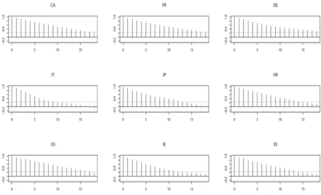
Functions (ACFs) in Figure 2.
Figure 1: Time-series for the real GDP per capita for a pool of advanced European economies are shown, spanning the period 1995q1 to 2016q4. They account for G7 economies (CA, FR, DE, IT, JP, UK, and US) and for two non-G7 European countries (IE and ES). TheY andXaxis represent the series and sampling time, respectively. All the series are expressed in quarters and seasonally adjusted. All data points are obtained from OECD data source.
A common model building strategy is to select the exact differentiation order and thus
plau-sible values of AR (p) and MA (q) lag orders on statistics calculated from the data to assess the
stationarity and invertibility of the process in (27) for each selected country. More precisely, I use
Figure 2: Sample Autocorrelation Functions for the real GDP per capita for a pool of advanced European economies are shown, spanning the period 1995q1 to 2016q4. They account for G7 economies (CA, FR, DE, IT, JP, UK, and US) and for two non-G7 European countries (IE and ES). The dashed lines display the Bartlett’s bands. TheY andX axis represent the ACFs values and lags, respectively. All lags are expressed in quarters.
(p) component (see, for instance, Schwarz (1978)) and the Augmented Dickey-Fuller (ADF) test in
equation (29) to choose the order of integration to ensure stationarity (see, for instance, Dickey
and Fuller (1979)).
B IC(p,q)=l og( ˆσ2)+(p+q)·l og(T)
T (28)
∆yt=α+βt+γyt−1+δ1∆yt−1+. . .+δp−1∆yt−p+1+ǫt (29)
where ˆσ2denotes the MLE ofσ2,αis a constant,βis the coefficient on a time trend, andpandq
denote the lag orders of the ARIMA process in (27).
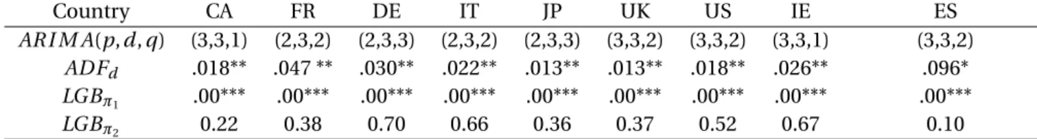
By equations (28) and (29), I estimate 9 different ARIMA processes. In Table 1, I display the
ARIMA time-series, the ADF tests in terms of p-values, and Ljung-Box test statistics of the series
to jointly assess the robustness of the estimates and investigate linear dependencies among
endogeneity issues.
Table 1: Estimates, Stationarity, and Diagnostic Test
Country CA FR DE IT JP UK US IE ES
AR I M A(p,d,q) (3,3,1) (2,3,2) (2,3,3) (2,3,2) (2,3,3) (3,3,2) (3,3,2) (3,3,1) (3,3,2)
ADFd .018** .047 ** .030** .022** .013** .013** .018** .026** .096*
LGBπ1 .00*** .00*** .00*** .00*** .00*** .00*** .00*** .00*** .00***
LGBπ2 0.22 0.38 0.70 0.66 0.36 0.37 0.52 0.67 0.10
The Table is so split: the first row displays the country indices; the second row refers to ARIMA(p,d,q) models; the third row stands for the ADF tests in terms of p-values and significant codes, withd=3; and the last two rows stand for Ljung-Box test statistics of the series (π1=p) and residuals (π2=q) in terms of p-values and significant codes. The significant codes are: *** significance at 1%, ** significance at 5%, and * significance at 10%.
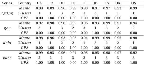
According to Bayesian inference, higher PMP distribution (equation (3)) and log Bayes Factor (equation (17)) among series are obtained by performing a BHFC procedure with a maximum
of three clusters (c=3). They are so split: (i) CA, FR, DE, IT, UK, US, and ES; (i i) IE; and (i i i)
JP. Table 2 shows the membership values and the corresponding cluster for each series8. The
findings address three important issues. First, when accounting for dynamics of the economy,
an accurate BMA strategy, as implied in BHFC procedure, is required in order to group dynamic
data objects into more probable homogenous clusters (Mτ). Second, the use of conjugate
hier-archical informative priors in fuzzy clustering algorithm is able to highlight similarity – in terms
of cross-country homogeneity – among series and thus group them in ’ad hoc’ clusters. Third,
membership values show the presence of relevant endogeneity issues (e.g., DE, FR, IT, CA, UK, SE, and US) and heterogeneity (e.g., JP and IE) among countries when performing fuzzy clustering of
time-series (Table 2). Finally, given the ROB strategy implied in the procedure9, the Conditional
Posterior Sign (CPS)10can be obtained by the Posterior Inclusion Probabilities11in order to
ob-serve how the GDP time-series for each country evolve over time. Most countries tend to show
negative effects (except for FR, JP, and ES) that, in a context of economic interactions and
interna-tional spillover effects, would be interpreted as net receivers given an unexpected shock on GDP.
Conversely, FR, JP, and ES seem to be net senders12. Thus, it would be interesting to extend the
fuzzy clustering analysis in a multivariate context (Section 7).
8I use Fuzzy C-Means with 2 parameter of fuzziness, 100 random starts of the algorithm, and 100 iterations per each
random start.
9See, for instance, Pacifico (2020b) for further specifications on the econometric methodology.
10The CPS refers to the posterior probability of a positive coefficient expected value conditional on inclusion. It
indicates a positive effect on GDP whether it is close to 1 and a negative effect whether it is close to 0.
11They correspond to the sum of PMPs between all the series according to their membership values. 12See, for instance, Pacifico (2019a).
Table 2: Membership Values and Clusters
Country MEMB1 MEMB2 MEMB3 Cluster CPS CA 0.001 0.992 0.007 2 0.007 FR 0.000 1.000 0.000 2 1.000 DE 0.002 0.989 0.009 2 0.028 IE 0.000 0.003 0.997 3 0.000 IT 0.002 0.985 0.013 2 0.000 JP 0.998 0.001 0.001 1 1.000 ES 0.010 0.838 0.152 2 0.979 UK 0.001 0.994 0.005 2 0.043 US 0.236 0.626 0.138 2 0.057 The Table is so split: the first column refers to the countries; the fol-lowing three columns display the membership values; the fifth col-umn displays the corresponding cluster membership; and the sixth column shows the CPSs.
The previous results are better highlighted graphically (Figure 3). Indeed, by focusing on the first cluster13, it is clear the presence of consistent heterogeneity among series, but with some
common components (e.g., DE, FR, IT, CA, and UK). However, a persistent homogeneity matters
over time among European countries, including US (misspecified dynamics). These findings
con-firm the efficacy of the BMA strategy implied in the BHFC with endogeneity issues when grouping
multiple dynamic processes. The remaining two clusters highlight that JP and IE series tend to
evolve in a heterogeneous way over time with respect to the others.
Figure 3: The real GDP per capita series are drawn and grouped according to the RWD measure, spanning the period 1995q1 to 2016q4. The three clusters are so split: (i) CA, FR, DE, IT, UK, US, and ES; (i i) IE; and (i i i) JP. TheY andX axis represent the series and sampling distribution in quarters, respectively.
In Table 3, I compare the performance of the BHFC procedure with some related distance
mea-sures14for effective clustering of ARIMA time-series: (i) the most natural metric for computing
13Here, the series ES and US have been dropped to better scale the plot. 14Own computations.
distance in most applications such as Euclidean Distance (ED)15; (i i) Dynamic Time Warping
(DTW)16; (i i i) Longest Common Sub-Sequence (LCSS)17; and (i v) Minimal Variance Matching
(MVM)18. Here, some considerations are in order. These clustering approaches would be
classi-fied as ’shaped-based similarity’ measures, suitable for short-length time-series and used to find
similar time-series in time and shape. More precisely, the ED measure is one of the most used
time-series dissimilarity measures, favored by its computational simplicity and indexing
capabil-ities. The DTW and LCSS approaches tend to be very appropriate in the case which the similarity between time-series is based on ’similarity in shape’ or there are time-series with different length.
They focus on the averaging method for time-series clustering and thus define a cluster by their
combinations hierarchically or sequentially. However, their drawback is the strong dependency
on the ordering of choosing pairs which result in different final clusters. Finally, MVM measure
computes the distance value between different time-series directly based on the distances of
cor-responding elements, just as DTW, and allows the query sequence to match to only subsequence
of the target sequence, just as LCSS. The main difference between LCSS and MVM is that LCSS
requires the distance threshold to optimize over the length of the longest common subsequence,
while MVM directly optimizes the sum of distances of corresponding elements without any dis-tance threshold. Instead, the main difference between DTW and MVM is that MVM is able to skip
some elements of the target series when computing the correspondence.
The main thrust of this example is to prove that RWD measure gets the higher cluster similarity
metric than the other related methods by dealing with either model uncertainty and overfitting
(implied in Bayesian framework) or endogeneity issues and misspecified dynamics (implied in
the BMA strategy) when clustering dynamic data. All approaches would perform better by
choos-ing two clusters. The JP series are grouped in a unique cluster with respect to the others (includchoos-ing
the IE series). By running the lBF (equation (17)) between the submodels Mτand the submodels
related to the alternative approaches (M∗)19, I find moderate support with DTW and MVM
mea-sures and strong evidence with LCSS measure by supporting elastic distances and unequal size
time-series in fuzzy clustering approach. No evidence (or weak support) is found for ED measure
due to its inability in clustering data sets containing many time series.
15See, e.g., Chan et al. (2003). 16See, e.g., Chu et al. (2002).
17See, e.g., Vlachos et al. (2002) and Banerjee and Ghosh (2001). 18See, e.g., Latecki et al. (2005).
19In this context, the submodels would correspond to the subsequences – which result in different clusters – between
time-series having maximum similarity with other objects within that group and minimum similarity with objects in other groups.
Table 3: Performance Comparison
Distance Measure Cluster CSM lBF Evidence
RWD 3 0.923 -
-ED 2 0.424 1.84 weak
DTW 2 0.594 5.07 moderate LCSS 2 0.763 7.13 strong MVM 2 0.605 5.49 moderate The Table is so split: the first column describes the distance measure used; the second column displays the optimal num-ber of clusters; the third column accounts for Cluster Similarity Metric; and the last two columns refer to the log Bayes Factor and the corresponding scale of evidence.
6.2 Simulated Example
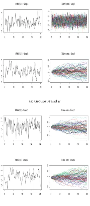
I perform fuzzy clustering on a database of ARIMA(1,1,1) time-series and analyze the results. More
precisely, I generate four groups (A, B,C, andD), each withk =75 ARIMA(1,1,1) time-series,
where t =1, 2, . . . , 200 and the parameter vectors (φ,θ) are uniformly distributed in the ranges [(1.30, 0.30)±0.01], [(1.34, 0.34)±0.01], [(1.60, 0.60)±0.01], and [(1.64, 0.64)±0.01], respectively. The
white noiseǫtused has mean zero and variance 0.01. All the simulated time-series are stationary,
invertible, and integrated of order one, AR I M A(1, 1, 1)∼I(1). I construct 10 collections from
these series and run fuzzy clustering on each of the groups. Collections 1−5 have been built by
selecting 15 time-series, each from groupsAandB. Similarly, collections 6−10 have been built
by selecting 15 time-series, each from groupsC andD(Figure 4).
According to Bayesian inference, higher PMP distribution (equation (3)) and log Bayes Factor
(equation (17)) among series are obtained by performing a BHFC procedure with a maximum of
three clusters (c=3).
In Table 4, I compare the cluster similarity metric obtained using RWD measure20with four dif-ferent traditional similarity measures21: (i) the most popular multidimensional scaling method
such as Weighted Euclidean Distance (WED)22; (i i) Discrete Wavelet Transform (DWT)23; (i i i)
Discrete Fourier Transform (DFT)24; and (i v) Principal Component Analysis (PCA)25. Here, some
considerations are in order. These clustering approaches would be classified as ’structural level’
20I use Fuzzy C-Means with 2 as parameter of fuzziness, 100 random starts of the algorithm, and 100 as maximum
iterations per each random start.
21Own computations.
22See, e.g., Horan (1969) and Carroll and Chang (1970). 23See, e.g., Struzik and Sibes (1999).
24See, e.g., Agrawal et al. (1993). 25See, e.g., Gavrilov et al. (2000).
(a) GroupsAandB
(b) GroupsCandD
Figure 4: Simulated ARIMA(1,1,1) time-series, withk=75 andt=200, from the groupsA,B,C, andD. TheY andX axis represent the series and sampling time, respectively.
similarity measures, based on global and high level structure and used for long-length time-series
data. More precisely, the WED depends on the combination of the weights used and the model
parameters. Thus, it tends to be more sensitive to the position of the AR coefficients and very close to the cepstral distance for effective clustering of ARIMA time-series. The DWT technique is
used in wide range of applications from computer graphic to speech, image, and signal
process-ing. The advantage of using DWT is its ability of representation of time-series as multi-resolution.
localization property of DWT. The DFT uses the Euclidean distance between time-series of equal
length as the measure of their similarity. Then, it reduces their sequences into points in
low-dimensional space. The approach tends to improve upon the measurement of similarity between
time-series since the effects of high frequency components, which usually correspond to noise,
are discarded. Finally, the PCA is a well-known data analysis technique widely used to measure
time-series similarity in multivariate analysis. The particular feature of PCA is the main tendency
of observed data compactly and thus the ability to be used as a method to follow up a clue when any significant structure in the data is not obvious. However, when the data does not have a
struc-ture that PCA can capstruc-ture, satisfactory results cannot be obtained due to the uniformity of the
data structure and thus any significant and accumulated proportion for the principal
compo-nents cannot be found.
The higher cluster similarity metric is found for the RWD measure (close to 1) and thus the
BHFC procedure is able to provide an accurate clustering for all of the ARIMA(1,1,1) collections,
by jointly dealing with endogeneity issues and structural model uncertainty, where one or more
parameters are posited as the source of model misspecification problems. The results also
indi-cate that the dynamic data objects are clustered with a high confidence level and thus the RWD measure would be better that the other distance measures.
Table 4: Cluster Similarity Metric
Collection RWD WED DWT DFT PCA 1 0.980 0.813 0.596 0.561 0.533 2 0.989 0.817 0.599 0.553 0.578 3 0.990 0.835 0.598 0.595 0.583 4 0.960 0.807 0.565 0.547 0.521 5 0.969 0.821 0.583 0.556 0.569 6 0.969 0.823 0.553 0.537 0.534 7 0.985 0.817 0.579 0.603 0.606 8 0.964 0.825 0.589 0.621 0.625 9 0.978 0.871 0.632 0.650 0.633 10 0.998 0.853 0.661 0.669 0.665 lBF - 8.45 6.71 6.57 1.33
Evidence - strong moderate moderate weak The Table shows the cluster similarity metric for five different distance measures. The columns display all of the ARIMA(1,1,1) time-series collections and the related distance measures used for the fuzzy clus-tering analysis. The last two columns refer to the log Bayes Factor and the corresponding scale of evidence, respectively.
In Appendix A, I draw the clustering plots accounting for all of the 10 collections from the
select-ing 15 time-series, each from groupsAandB. The others (6−10) have been built by selecting 15
time-series, each from groupsCandD. All the grouped series show a highly low average
dissim-ilarity within a cluster and a highly strong dissimdissim-ilarity between clusters. Thus, the three clusters
are well defined and separated. In addition, given the BMA implied in the BHFC procedure,
dy-namics between series are well highlighted and grouped. By plotting all of the ARIMA(1,1,1)
col-lections within each cluster, these dynamics are better observed and, in a context of multicountry
setups, they would correspond to time-varying cross-country linkages such as interdependence, heterogeneity, and commonality (Figure 10 in Appendix B).
7 RWD Measure in High Dimensional Time-Varying Multicountry Data
In this section, I extend the analysis to Vector Autoregressive (VAR) models in order to test the
per-formance of the BHFC procedure when investigating endogeneity issues, misspecified dynamics,
and linear interdependencies among multiple time-series.
The empirical application builds on Pacifico (2019a) and focuses on a simplified version of the SPBVAR accounting for 9 advanced countries, the G7 economies [Canada (CA), France (FR),
Ger-many (DE), Italy (IT), Japan (JP), the United Kingdom (UK), and the United States (US)] and two
non-G7 European countries [Ireland (IE) and Spain (ES)], and some of the core variables of the
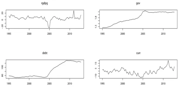
real [real GDP growth rate (r g d pg) and general government spending (g ov)] and financial
[gen-eral government debt (d ebt) and the current account balance (cur r)] business cycles. The overall
series are expressed in quarters and all data points are originated from the OECD database (Table
6).
The simplified version of the time-varying SPBVAR developed in Pacifico (2019a) takes the form:
Yi tm¨=Ami t¨,j(L)Yi,tm¨−1+ε¨i t (30)
wherei,j=1, 2, . . . , 9 are country indices,t =1, 2, . . . ,T denotes time, ¨m=1, . . . , 4 denotes the set
of endogenous variables, Ai t,j is a 36·36 matrix of real and financial variables for each pair of
countries (i,j) for a given ¨m,Yi,t−1is a 36·1 vector of lagged variables of interest that accounts for
the real and financial dimensions for eachifor a given ¨m, and ¨εi t∼i.i.d.N(0, ¨Σ) is an 36·1 vector
of disturbance terms. For convenience, I suppose one lag and no intercept.
with-out restrictions, to 3, 168 regression parameters. More precisely, each equation of the time-varying
SPBVAR in (30) has 36 coefficients and there are 88 equations in the system. According to the BMA
strategy implied in the BHFC procedure, there are 236=68, 719, 476, 736 possible model solutions.
Thus, it is very costly to select subsets of clusters (Mτ) via MCMC algorithms since the number of
coefficients is increased byNM¨ factors, with ¨Mdenoting the set of the lagged endogenous
vari-ables accounted for. Moreover, all series vary over time and thus dynamic relationships, cross-unit
lagged interdependencies, and dynamic feedback matter. Then, in order to be able in applying the specifications underlying the BHFC procedure (Section 4), I need to express the time-varying
SP-BVAR in (30) in terms of a multivariate normal distribution.
By adapting the framework of Pacifico (2019a) and following the Bayesian implementations in
Pacifico (2020b), I can able to express the time-varying SPBVAR in terms of multivariate normal
distribution: Yt=(INM¨⊗X¨t) ¨γt+E¨t (31) whereYt=(Ym¨ ′ 1t , . . . ,Y ¨ m′ N t) ′
is an 36·1 vector containing the set of real and financial variables for
each i for a given ¨m, ¨Xt =(Y
′m¨ i,t−1,Y ′m¨ i,t−2, . . . ,Y ′m¨ i,t−l) ′
is an 1·k¨ vector containing all lagged vari-ables for eachi, with ¨k =NM¨ be the number of all matrix coefficients in each equation of the
model (30) for each pair of countries (i,j), ¨γki t,¨ j=vec( ¨gi tk¨,j) is anNM¨k¨·1 vector containing all
columns, stacked into a vector26, of the matrix At(L) for each pair of countries (i,j) for a given ¨ k, and ¨Et=(¨ε ′ 1t, . . . , ¨ε ′ N t) ′
is an 36·1 vector containing the random disturbances of the model. In
model (31) there is no subscriptisince all lagged variables in the system are stacked in ¨Xt.
In this study, the implementation is adapted to the thrust of the RWD measure in merging more
similar MCs and thus identifying – as fast as possible – more probable homogeneous modelsMτ
among dynamic data. More precisely, the coefficient vectors in ¨γt represent all the model
solu-tions counted in the natural model spaceM (equation (7)), and each factor would correspond
to a clustering modelMτidentifying a distinct cluster of (potential) combination of the series ¨m.
The underlying logic is to exploit the Bayesian hierarchical framework implied in the BHFC
proce-dure in order to extend the clustering analysis by dealing with misspecified dynamics (structural
uncertainty) and endogeneity issues when studying and conducting fuzzy clustering analysis in
26Here, the vec operator is used to transform a matrix into a vector by stacking the columns of the matrix one
under-neath the other, with ¨gi tk¨,j=(A1i t′,j,Ai t,j2′ , . . . ,AMi t,j¨′ )′and ¨γt=( ¨γ ′ 1t, ¨γ ′ 2t, . . . , ¨γ ′ N t) ′
denoting the time-varying coefficient vectors, stacked fori, for each country–variable pair.
time-varying multicountry setups. However, because the coefficient vectors in ¨γtvary in different
time periods for each country–variable pair and there are more coefficients than data points, to
avoid the dimensionality problem, I adapt the framework in Pacifico (2019a) and assume ¨γt has
the following factor structure:
¨ γt= ¨ F X f=1 ¨ Gf·βf t¨ +u¨t with u¨t∼N(0,Σu)¨ (32)
where ¨F ≪NM¨k¨ andd i m(βf t¨)≪d i m( ¨γt) by construction, ¨Gf¨=[ ¨G1, ¨G2, . . . , ¨GF¨] are NM¨k¨·1
matrices obtained by multiplying the matrix coefficients ( ¨gi tk¨,j) stacked in the vector ¨γt by
con-formable matricesB¨
f with elements equal to zero and one27,ut is anNM¨k¨·1 vector of unmod-elled variations present in ¨γt, andΣu¨=Σe¨⊗V¨, whereΣe¨is the covariance matrix of the vector
¨
Et and ¨V =(σ2Ik¨) as in Kadiyala and Karlsson (1997). The idea is to shrink ¨γt to a much smaller
dimensional vectorβt, withβt =(β
′ 1t,β ′ 2t, . . . ,β ′ ¨ F t) ′
denoting the adjusted auxiliary indicator
de-fined in Section 4 (β={βk}), and containing all regression coefficients stacked into a vector.
Running equations (31) and (32) for the model described in (30), I assume that the coefficient
vectors in ¨γtdepends on three factors:
¨
Gf¨βf t¨ =G¨1β1t+G¨2β2t+G¨3β3t+u¨t (33)
where, stacking fort,βf¨=(β1,β2,β3)
′
contains all the series to be estimated and grouped in dis-tinct clusters for each clustering modelMτ. Given the factorization in equation (33), the
reduced-form SPBVAR model in equation (31) can be transreduced-formed into a Structural Normal Linear
Regres-sion (SNLR) model28written as
Yt=Θ¨t µ 3 X ¨ f=1 ¨ Gf¨βf t¨ +u¨t ¶ +E¨t≡χ¨f t¨βf t¨ +η¨t with Θ¨t= ³ INM¨⊗X¨t ´ (34)
where ¨Θt contains all the lagged series in the system by construction, ¨χ¨
f t≡Θ¨f t¨ G¨f t¨ is anNM¨·1 matrix that stacks all coefficients of the system, and ¨ηt ≡Θ¨f t¨ u¨t+E¨t ∼N(0,σt·Σu¨), withσt =
(IN+σ2Θ¨
′
tȨt).
27Here,B ¨
f would correspond to the auxiliary indicatorβ=(βk) in matrix form.
28See, for instance, Pacifico (2019b) for an illustration of the conformation of the time-varying multicountry SPBVAR