Unequal Edge Inclusion Probabilities in Link-Tracing Network Sampling With Implications for Respondent-Driven Sampling

(1)

Smith ScholarWorks

Statistical and Data Sciences: Faculty

Publications

Statistical and Data Sciences

2016

Unequal Edge Inclusion Probabilities in Link-Tracing Network

Sampling With Implications for Respondent-Driven Sampling

Miles Q. Ott

Augsburg College, [email protected]

Krista J. Gile

University of Massachusetts Amherst

Follow this and additional works at: https://scholarworks.smith.edu/sds_facpubs

Part of the Categorical Data Analysis Commons, and the Other Mathematics Commons

Recommended Citation

Ott, Miles Q. and Gile, Krista J., "Unequal Edge Inclusion Probabilities in Link-Tracing Network Sampling With Implications for Respondent-Driven Sampling" (2016). Statistical and Data Sciences: Faculty Publications, Smith College, Northampton, MA.

https://scholarworks.smith.edu/sds_facpubs/9

This Article has been accepted for inclusion in Statistical and Data Sciences: Faculty Publications by an authorized administrator of Smith ScholarWorks. For more information, please contact [email protected]

(2)

Vol. 10 (2016) 1109–1132 ISSN: 1935-7524

DOI:10.1214/16-EJS1138

Unequal edge inclusion probabilities in

link-tracing network sampling with

implications for Respondent-Driven

Sampling

Miles Q. Ott

Augsburg College Mathematics and Statistics Department 2211 Riverside Avenue, Minneapolis MN 55454

and Krista J. Gile

Department of Mathematics and Statistics, University of Massachusetts, Amherst Abstract: Respondent-Driven Sampling (RDS) is a widely adopted link-tracing sampling design used to draw valid statistical inference from sam-ples of populations for which there is no available sampling frame. RDS estimators rely upon the assumption that each edge (representing a rela-tionship between two individuals) in the underlying network has an equal probability of being sampled. We show that this assumption is violated in even the simplest cases, and that RDS estimators are sensitive to the violation of this assumption.

Keywords and phrases:Respondent-driven sampling, link tracing, net-work sampling, edge inclusion, random walk.

Received June 2015.

1. Introduction

This paper demonstrates that variants of without-replacement link-tracing net-work sampling result in a non-uniform distribution of sampling probabilities of network edges. This is of particular interest because common estimators for the widely-used respondent-driven sampling (RDS, [9]) method rely on the as-sumption of equal edge sampling probabilities. In this paper, we show that under without-replacement link-tracing sampling, edge-sampling probabilities are non-uniform, that edges incident to higher degree vertices tend to be sampled less often, and that this issue can induce bias in the widely-used RDS estimator [18]. We also elaborate further properties of this phenomenon.

Respondent-driven sampling [9] is a variant of a link-tracing network sampling procedure [8]. In link-tracing, a few units of the target population are sampled as ‘seeds’, and links from current samples are iteratively followed to enlarge the sample. Variants of link-tracing, often referred to as snowball sampling [7,

(3)

8], are often used to sample hard-to-reach human populations, leveraging the social connections of the target population to enlarge the sample beyond the subgroup known to researchers. The resulting sample, however, is typically not a probability sample and results in highly unequal sampling probabilities.

The RDS variant of link-tracing, introduced by Heckathorn [9, 10], is dis-tinguished by the fact that sampling is conducted by the respondents, who are given a small number of uniquely-identified coupons to distribute among their un-sampled contacts in the target population. The coupon mechanism results in reduced confidentiality concerns in sensitive populations, and the small number of coupons controls branching so that the sample reaches many steps from the original (convenience) sample of seeds for finite sample size, reducing sample dependence on the seeds, making it more reasonable to treat the final sample as a probability sample.

RDS is extensively used in public health research to study populations that are at an elevated risk for adverse health events. In HIV surveillance, RDS has been used extensively in populations of people who inject drugs, commercial sex workers, and men who have sex with men [16, 15, 12], as it is not prac-tical to sample from these populations through conventional means. RDS has therefore been used to study HIV prevalence and other population characteris-tics in hundreds of studies around the world, often with critical public health implications.

We begin this paper in Section2by relating the assumption of uniform edge sampling probability to inference from RDS data. Section3explores this result analytically. For a special class of networks, we are able to make more defi-nite statements of relative edge sampling probabilities for non-branching edge sampling in Section4. In Section5, we investigate the equal edge sampling prob-ability assumption for five specific networks with varying structures, assuming a non-branching process. In Section 6we return to branching structures approx-imating RDS sampling, illustrate that our analytical results in non-branching sampling apply to these structures, and demonstrate that this phenomenon can lead to bias in estimation from RDS data. We conclude with a discussion in Section7. Throughout the paper we assume a simple undirected graph with no parallel edges or self-loops.

2. RDS inference and uniform edge sampling assumption

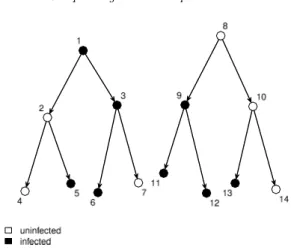
Figure 1 illustrates a hypothetical RDS recruitment tree. This sample starts with two seeds {1,8}, and each participant recruits another two participants. Participants are sampled without replacement. In this way, RDS proceeds as a branching link-tracing sample [9,4].

Despite the branching without-replacement structure of true RDS samples, most work in RDS [22, 18] approximates the RDS sampling procedure as a with-replacement random walk sampling vertices along their incident network edges.

This random walk is modeled as a Markov chain on the state space of vertices. If thedegree of vertexi, di is the number of edges incident toi, the transition

(4)

Fig 1_._{Illustration of Hypothetical RDS Recruitment Tree}

matrix is then T = {Tij}, where Tij = di1 if i and j are connected, and 0 otherwise. The stationary distribution of this Markov chain is proportional to vertex degree: πi = αdi, for constant α. It is therefore understood that the marginal vertex-wise sampling probabilities (marginalizing over all choice of seeds and all sample paths) in RDS are unequal, and most common estimators either directly use [22,18] or adapt [5,3] probabilities proportional to degrees. In this setting, we can also consider the stationary distribution edge sampling probabilities. IfPk(i→j) is the probability of transitioning from vertexito ver-texj at stepk, this is given byP(kth sample isi)_di1, which, under stationarity, takes the value αdi_di =α, equal for all edges of the network.

Though the with-replacement sampling assumption of this approximation is known to be false, this assumption is required by the estimators in [18] and [22]. Gile [3], Gile and Handcock [4], Lu et al. [14] illustrate how large sample fractions can create substantively impactful violations of this assumption in the estimator in [22]. Gile and Handcock [4] also suggests the estimator in [18] is subject to bias in the case of large sample fractions, but does not suggest why. In this paper, we clarify that this bias is due to the unequal edge-sampling probabilities induced by without-replacement sampling.

The estimator proposed by Salganik and Heckathorn [18] relies on the as-sumption of equal edge sampling probabilities, arguing that for a low sample fraction, the with-replacement approximation is adequate. Thompson [20] claims that these sampling probabilities are not equal for without-replacement sam-pling. In this paper, we show that this approximation is inadequate in many cases, and accounts for the ﬁnite population bias of the estimator in Salganik and Heckathorn [18].

(5)

3. Analytical consideration of unequal edge-sampling probabilities

Properties of random walks have been studied extensively in the graph theory literature (e.g. [6,13]). Self-avoiding random walks on lattices are of particular interest in Physics and Chemistry [1,2], where the interest is in characterizing the random walk by determining properties of the self avoiding random walk (such as the distribution of end-vertex, mean-square length, etc) however we are unaware of any research on the edge sampling probabilities of self-avoiding random walks on non-lattice graphs. In this section we analytically explore prop-erties of self-avoiding random walks. In particular, we will derive propprop-erties of edge sampling probabilities for without replacement random walks on arbitrary graphs. Proofs for the theorems and corollaries in this section are provided in the appendix.

Consider an undirected networkG={V, E}, whereV is the vertex set, and

E is the edge set. Each edge is a pair of vertices such that the vertices share a relationship of interest, where the edge between vertex 1 and vertex 2 is denoted (v1, v2). Let theneighborhoodofi, denotedN(i), be the set of all vertices with

which vertexishares an edge. Finally, for nodal degrees{di}, letd=

idi. Consider a random walkS={S1, S2, . . .}on the vertices of undirected graph

G, whereSiis the random variable for the index of the vertex visited at theith step. LetPk(i) denoteP(Sk =i). We begin by deﬁning edge passage probabili-ties.

Deﬁnition 1. Thek-step directed passage probabilityof vertex pair(i, j)∈

E is the probability that thekth _{observed passage originates at vertex}_i_and

ter-minates at vertexj along edge(i, j). This probability is denotedPk(i→j). Deﬁnition 2. The k-step undirected passage probability of undirected edge (i, j) ∈ E is the probability that the kth observed passage traverses edge

(i, j)in either direction. This probability is denotedP_k(i→j), andP_k(i→j) =

Pk(i→j) +Pk(j→i).

We first show that in the first few steps of a without-replacement random walk beginning at with-replacement stationarity (the first vertex is chosen with probability proportional to degree), edge sampling probabilities look very similar to those of with-replacement random walks. In particular, each edge is equally likely to be sampled in the first or second edge passage.

Theorem 1. Consider a without replacement (self-avoiding) random walk on an undirected network with minimum degree 2. LetS1be chosen with probability

proportional to degree. That is, P1(s1) = ds_d1. Then P1(s1 → s2) = P2(s2 →

s3) =1_d for all(s1, s2)and(s2, s3)∈E.

Several other results follow from Theorem 1 (with proof in the appendiz). Since we know the exact directed edge sampling probabilities for the first and second edges, we can also derive the exact undirected edge sampling probabilities for the first and second edges, again assuming that the first vertex is sampled with probability proportional to degree.

(6)

Corollary. P₁(s1→s2) =P2(s2→s3) = 2_d for all(s1, s2)and(s2, s3)∈E.

In addition to analytically determining the edge sampling probabilities for the ﬁrst two edges, we can also analytically ﬁnd the vertex sampling probability for the second vertex in the random walk.

Corollary. P2(s2) =

ds₂

d for alls2∈V.

Again following from Theorem1, we can show that when the ﬁrst vertex is chosen with probability proportional to degree then each vertex has probability proportional to degree of being the third vertex in the non-repeating random walk.

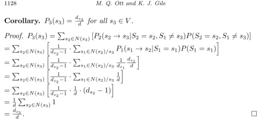
Corollary. P3(s3) =ds_d3 for alls3∈V.

Thus far we have proved results for the ﬁrst two steps of without-replacement random walks that are identical to those for their with-replacement counter-parts. We establish that these results do not hold for the third sampled edge in the theorem below, proved in the appendix:

Theorem 2. There exists a graph Gfor whichP3(s3→s4)= 1_d.

4. Unequal probabilities for isolate join complete graphs

In the previous section we showed that the third edge probability depends upon the graph structure. Here we introduce a class of graphs for which it is possible to evaluate P3(i→j)> _d1, given that we knowdi and dj. Consider a graphG where q > 3 vertices are maximally connected, meaning each of these vertices shares an undirected edge with every other vertex in the graph. Furtherw >1 vertices only share edges with theqmaximally connected vertices. We will refer to these vertices as minimally connected. In total there are q +w vertices, where the maximally connected vertices all have degree q−1 +w, and the minimally connected vertices have degreeq. We call this class of graphsIsolate Join Completegraphs or IJC since they are formed by joiningwisolates with a

q complete graph.

In this section we will concern ourselves with deriving the probabilities of the third edge traversed on a without replacement random walk of an IJC graph when the initial vertex is chosen in proportion to degree. Speciﬁcally, we treat the three equivalence classes of edges in such a network: when the third edge is between two maximally connected vertices, when the third edge goes from a minimally connected vertex to a maximally connected vertex, and when the third edge goes from a maximally connected vertex to a minimally connected vertex. Note that there are no edges connecting two minimally con-nected vertices. We are able to show that the third edge of a random walk is more likely to transverse an edge incident to a vertex with a lower de-gree.

While the topology ofGwould be unlikely to occur in practice, this example allows us to derive the sampling probabilities of the third edge, conditional

(7)

on the degree of the incident vertices, which would be impossible to do for any realistic graph. We address this limitation in lack of generalizability by including simulations on graphs that are more realistic in Sections5and6.

4.1. Analytic results

First we consider the third edge between two maximally connected vertices, and provide proofs for this and the other theorems in the appendix. In an IJC graph we are interested in ﬁnding theP3(s3→s4) where boths3ands4are maximally

connected vertices.

Theorem 3. P3(s3→s4)< 1_d whens3, s4 are maximally connected vertices in

an IJC graph.

Next we consider the third edge from a maximally connected vertex to a minimally connected vertex. Speciﬁcally, in an IJC graph we are interested in ﬁnding the P3(s3 → s4) where vertex s3 is maximally connected with degree

w+q−1 and vertexs4is minimally connected with degreeq.

Theorem 4. P3(s3→s4)>1_d whens3is a maximally connected vertex and s4

is a minimally connected vertex in an IJC graph.

Finally, we consider the third edge from a minimally connected vertex to a maximally connected vertex. In an IJC graph we are interested in ﬁnding the

P3(s3 →s4) where vertex s3 is minimally connected with degreeq and vertex

s4 is maximally connected with degreeq+w−1.

Theorem 5. P3(s3 → s4) = 1_d when s3 is minimally connected and s4 is

maximally connected in an IJC graph.

Thus, we have shown that for this special class of networks which allow for analytics, the third step of a without-replacement random walk is less likely to sample edges incident to two higher degree vertices. In the subsequent sections, we illustrate that this trend is consistent with later steps of the random walk, and with more general network structures.

5. Comparison across network structures

We showed analytically that in an IJC graph, edges that are between two high degree vertices are least likely to be sampled in without-replacement random walks after the second step. To further demonstrate that this phenomenon is not speciﬁc to those idealized networks, we performed simulations of without replacement random walks on several diﬀerent networks: an Erdos-Renyi net-work with 100 vertices, an Erdos-Renyi netnet-work with 10,000 vertices, an IJC network, Zachary’s Karate Club network [24], and the Colorado Springs network [17].

In each set of simulations, we consider a without replacement non-branching random walk, beginning with a vertex selected with probability proportional to

(8)

degree, with each subsequent vertex chosen completely at random from among the un-sampled incident vertices of the previous vertex. The random walk con-tinues until there are no candidate subsequent samples available, or until the desired maximum sample is obtained. The directed edges sampled (traversed) are the edges joining each consecutive pair of vertices in the sample. In partic-ular, we consider the degree of the vertex at each end of a sampled edge. We refer to the degree of the ﬁrst vertex in the sequence as thesend degreeand the degree of the second as thereceive degree. We simulate 10 million such without replacement random walks on each example network, and record the sampling rates of edges with various incident degrees. We describe each network in more detail before presenting simulation results.

The 100 vertex Erdos-Renyi network was formed with probability that vertex

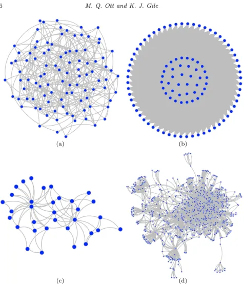
i and vertex j share an edge equal to 0.07, for all vertices. In the particular network we used in the simulations below, this resulted in a network with a total of 344 edges. The mean degree in the network is 6.88, the minimum degree is 3, and the maximum degree is 14. This Erdos-Renyi network is visualized in Figure2(a).

The 10,000 vertex Erdos-Renyi network was formed with probability that vertex i and vertex j share an edge equal to 0.0017, for all vertices. In the particular network we used in the simulations below, this resulted in a network with a total of 85,206 edges. The mean degree in the network is 17.04, the minimum degree is 4, and the maximum degree is 36.

The IJC network was also formed on 100 vertices, with 40 vertices that are maximally connected (q = 40), and 60 vertices that are minimally connected (w= 60). This network is visualized in Figure2(b).

Zachary’s Karate Club network [24] represents social relations between 34 members of a karate club. We treated a binary undirected version of this net-work, treating a tie in either direction, of any weight as an edge. We also removed one vertex that had degree one. This resulted in a network with 77 edges, mean degree 4.67, minimum degree 2, and maximum degree 17. The karate club net-work is visualized in Figure2(c).

The Colorado Springs network [17] represents social relations between het-erosexual adults who were identiﬁed at being at high risk for contracting HIV. As with Zachary’s Karate Club network, we also treated a symmetrized ver-sion of this network, treating a nomination in either direction as an edge. We considered the largest connected component, and successively removed vertices of degree of one until all vertices have at least degree two. Once modiﬁed, this network has a total of 2813 undirected edges and 822 vertices. The mean degree is 6.84, the minimum degree is 2, and the maximum degree is 100. The Colorado Springs network is visualized in Figure 2(d).

5.1. Simulation results

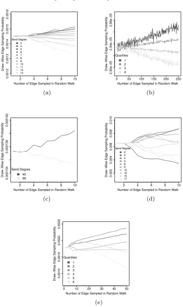
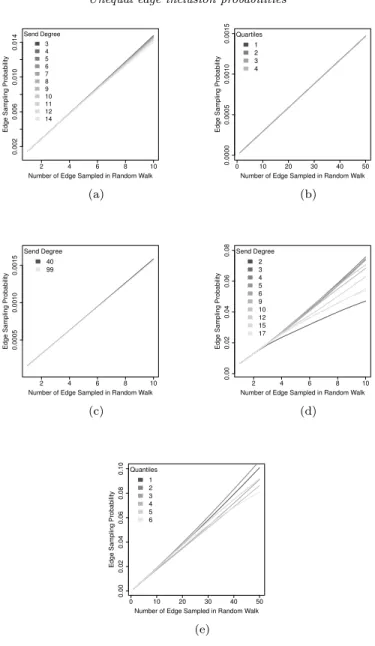
We display the draw-wise probability of sampling an edge by send degree in Figure3, and by receive degree in Figure4. Consistent with our analytic deriva-tions in Section 3, we see that for the ﬁrst two edges traversed in our without

(9)

Fig 2_{. Four Networks (The Erdos-Renyi network on 10,000 vertices is not pictured): (a)}

Erdos-Renyi on 100 vertices; (b) IJC on 100 vertices; (c) Zachary’s Karate Club Network; and, (d) Colorado Springs Network.

replacement random walk, each edge has the same probability of being sampled, regardless of incident degrees or network structure. However, as the without re-placement random walk continues to three or more edges, the probability of an edge being sampled begins to diverge. The edge sampling probabilities of the IJC network in Figures3(c) and4(c) which only has two kinds of vertices (those with degree 99 and those with degree 40) is perhaps simplest to interpret. As more edges are traversed, the edges incident to vertices with degree 40 (whether as send or receive degree) have an increasing chance of being sampled, while the edges that are incident to vertices with degree 99 have a decreasing chance of being sampled. This inverse relationship between degree of incident vertex and edge sampling probability also seems to hold for the other four networks.

(10)

Fig 3_{. Draw-wise Edge Sampling Probability by Send Degree for Five Networks: (a)}

Erdos-Renyi on 100 vertices; (b) Erdos-Erdos-Renyi on 10,000 vertices; (c) IJC on 100 vertices; (d) Zachary’s Karate Club Network; and, (e) Colorado Springs Network.

However, there are exceptions to this pattern of an inverse relationship be-tween degree of incident vertex and edge sampling probability. Most notably, when looking at the edge sampling probabilities bysenddegree in the Zachary’s Karate Club network in Figure 3(d) we see that edges with degree 2 have the lowest probability of being sampled after the ﬁrst two edges are sampled. This aberration can be easily explained. With the simulations on Zachary’s Karate

(11)

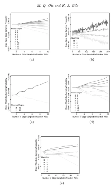
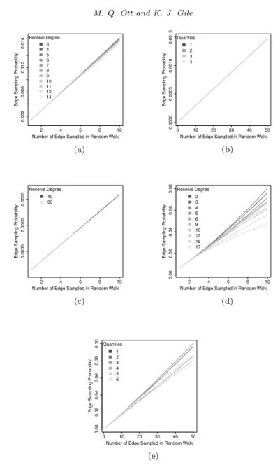
Fig 4_{. Draw-wise Edge Sampling Probability by Receive Degree for Five Networks: (a)}

club, each non-repeating random walk continued either until 10 edges were sam-pled, or until the walk could not continue without repeating a vertex. When a vertex with degree 2 is sampled later on in the non-repeating random walk, the probability that there are no un-sampled vertices in its neighborhood is quite high, and therefore the random walk is likely to end on a vertex with degree 2. This results in edges with a send degree 2 having a lower probability of being sampled.

(12)

Fig 5_{. Cummulative Edge Sampling Probability by Send Degree for Five Networks: (a)}

We also display the simulation results looking not at the draw-wise edge sampling probability, but the cumulative edge sampling probability (i.e. has the edge been sampled anytime before and including stepk?) both by send degree (Figure 5) and receive degree (Figure 6). Again, the edges incident to lower degree vertices (represented by darker colors) tend to have a higher cumulative probability of being included in the without replacement random walk than the

(13)

Fig 6_{. Cumulative Edge Sampling Probability by Receive Degree for Five Networks: (a)}

edges incident to higher degree vertices (represented by lighter colors), especially as the random walk increases in length.

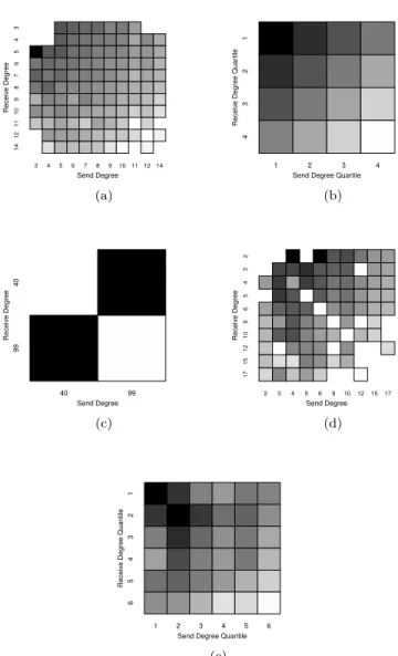
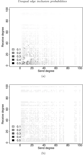
Finally we consider both the send degree and receive degree simultaneously in heatmaps in Figure 7. In these heatmaps higher probabilities are denoted with darker colors while lower probabilities are denoted with lighter colors. We see that edges that are incident to two low degree vertices tend to have

(14)

Fig 7_{. Cumulative Edge Sampling Probability Heatmaps for Five Networks: (a) Erdos-Renyi}

on 100 vertices, 10 edges sampled; (b) Erdos-Renyi on 10,000 vertices, 250 edges sampled; (c) IJC on 100 vertices, 10 edges sampled; (d) Zachary’s Karate Club Network, 10 edges sampled; and, (e) Colorado Springs Network, 50 edges sampled.

the highest probability of being included in the without replacement random walk, edges incident to one high degree vertex and one low degree vertex have lower probability, and edges incident to two high degree vertices have lowest probabilities, across network structures. All walks have 10 edges sampled, except for the walks on the 10,000 vertex Erdos-Renyi network (250 edges) and the Colorado Springs network (50 edges).

(15)

6. Implications of unequal edge sampling probabilities

The premise of uniform edge sampling probability underlies many diﬀerent facets of estimation and diagnostic assessments of RDS. In this section we in-troduce one of the most commonly implemented RDS prevalence estimators, the Salganik-Heckathorn (SH) estimator [18], then explore how falsely assum-ing uniform edge samplassum-ing probabilities can induce bias in the SH estimator of prevalence.

6.1. The Salganik-Heckathorn estimator

The SH estimator uses information on the number of between-group ties in an RDS sample. For instance, suppose population group A is comprised of those who are HIV positive, while groupBis comprised of those who are HIV negative. We consider the case where we are interested in estimating the proportion of a networked-population that is HIV positive P(A). Suppose we know T(BA) is

the average number of ties each HIV negative person has to someone who is HIV positive, andT(AB)is the average number of ties each HIV positive person

has to an HIV negative person. Since we assume the network is undirected the total number of ties from someone who is HIV negative to someone HIV positive must equal the total number of ties from someone HIV positive to someone HIV negative. Therefore, if T(AB) =a·T(BA) then there must bea times as many

people who are HIV negative than HIV positive. Using this equality, we can use the average number of cross-ties from each group to ﬁnd the prevalence of HIV which we denote asP(A):

P(A)=

T(BA)

T(BA)+T(AB)

.

By symmetry we also have that:

P(B)=

T(AB)

T(AB)+T(BA)

.

Next we substituteD(B)·C(BA) forT(BA)andD(A)·C(AB)forT(AB)where

D(B) is the average degree for those who are HIV negative and C(BA) is the

proportion of ties incident to HIV negative nodes that go to HIV positive nodes. Then we have:

P(A)=

D(B)·C(BA)

D(B)·C(BA)+D(A)·C(AB)

.

If the entire network structure and the HIV status of each member of the pop-ulation were known, we wouldn’t need to perform RDS. Salganik and Heckathorn [18]’s method involves performing RDS, while keeping track of the between and within group referrals and the degree for each participant sampled. They esti-mate:

C(AB)=

r(AB)

(16)

C(BA)=

r(BA)

r(BA)+r(AA)

,

where r(AB) is the number of referrals from someone who is HIV positive to

someone who is HIV negative, r(AA) is the number of referrals from someone

who is HIV positive to another person who is HIV positive, and so on. Further,

D(A)andD(B)are also unknown and need to be estimated in order to compute

prevalence estimates. The SH estimator uses the generalized Horvitz-Thompson [11, 19] estimator to estimate the average degree for the positive and negative groups, assuming sampling probabilities are proportional to reported degrees:

D(A)= n(A) n i=1 1 diI(Ai) D(B)= n(B) n i=1diI1(Bi) ,

where n(∗) is the number of observed vertices in class ∗. Then the estimator takes the form:

P(A)= D(B)×C(BA) D(B)×C(BA)+D(A)×C(AB) P(B)= D(A)×C(AB) D(A)×C(AB)+D(B)×C(BA) .

The SH estimator out-performs other estimators in certain situations, partic-ularly when there is differential recruitment effectiveness [21]. However, the SH estimator has been noted to perform poorly in the presence of differential activ-ity (when infected individuals have different average degree than non-infected individuals), and when there is a large sample fraction [4, 21,5].

6.2. Simulation study on eﬀect of without-replacement sampling on SH estimator

In order to further demonstrate the bias that is incurred in the SH prevalence estimator, we simulated RDS on the Colorado Springs network. The Colorado Springs Network dataset includes information on which individuals are involved in sex work (either as a sex worker or as a pimp), and we used involvement in sex work as the binary outcome of interest, treating those involved in sex work as groupAand those not involved in sex work as groupB. As above, we limited our analyses of the Colorado Springs network to the largest connected component, treated all edges as undirected, and deleted vertices that had degree less than 2, resulting in a network (Figure 2(d)), with 822 vertices and 2813 undirected edges. Those who were involved in sex work accounted for 9% of the vertices and had an average degree of 8.12, while those who were not involved in sex work had an average degree of 6.72.

(17)

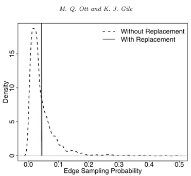
Fig 8_{. Edge Sampling Probabiltiy Densities on the Same Network when sampling is with and}

without replacement.

RDS was simulated by starting with 2 seeds chosen with probability propor-tional to degree, and allowing each vertex to refer up to two adjacent previously-unsampled vertices, until the sample size reached 250 vertices. We repeated this procedure 1,000,000 times. For each of the 1,000,000 simulations performed on the same network described above, we kept track of which vertices were sampled, which edges were sampled, and calculated the SH prevalence estimates for sex work involvement, P(A). We also calculated C(AB) andC(BA), as well as D(A)

andD(B). We then repeated these simulations with the key diﬀerence that we

allowed for visiting the same vertex more than once, in other words, we allowed RDS to proceed with-replacement.

If edges incident to higher degree vertices have a lower probability of being included in a sample, we would expect to see thatC(BA) will be an

underesti-mate,C(AB) will be an over estimate, and consequentlyP(A) will be an under

estimate, when RDS sampling is without replacement. 6.3. Simulation results

Earlier in this paper we demonstrated edges incident to higher degree vertices have a lower probability of being sampled in a non-branching without replace-ment random walk. In these simulations, we now are investigating a branching process both with and without replacement. Figure8 displays the densities of the cumulative edge sampling probabilities for each of the 2813 edges from the 1,000,000 simulations with and without replacement on the Colorado Springs network. The distribution of edge sampling probabilities is narrower,

(18)

symmet-Fig 9_{. Cummulative Edge Sampling Probability Heatmaps Under Two Conditions: (a)}

With-out Replacement; (b) With Replacement.

ric, and uni-modal when sampling with replacement, and markedly wider, right-skewed and bimodal when sampling without replacement.

Figures 9(a) and 9(b) present heatmaps of the cumulative edge sampling probabilities for the without replacement and with replacement simulations by send (recruiter) degree on the x-axis and receive (recruitee) degree on the y-axis. In these heatmaps, higher probability edges are denoted by darker colors, while lower probability edges are denoted by lighter colors. In Figure9(a) (where sampling is without replacement) it is apparent that edge sampling probabilities

(19)

Table 1

Error Rates of Simulated RDS With and Without Replacement MSE×103 |Bias| ×103 SE×102 Estimator w/ R w/o R w/ R w/o R w/R w/o R

P(A) 1.54 0.46 0.87 10.92 3.93 1.85 C(AB) 5.70 2.48 9.13 13.34 7.50 4.79 C(BA) 1.54 0.38 1.75 14.63 3.92 1.29 D(A) 26793.38 9313.93 168.66 286.33 491.21 105.61 D(B) 1212.88 4831.99 185.25 2193.27 108.56 14.69

vary by degree of incident vertices, where edges incident to receivers with lower degrees have a higher edge sampling probability. In Figure9(b) (where sampling is with replacement) there is no discernible relationship between edge sampling probabilities and the degrees of the incident vertices, as we would expect.

Having established that edges incident to higher degree vertices have a lower sampling probability, we next investigated how these non-uniform edge inclusion probabilities impact prevalence estimation with the SH estimator. In Table 1

we compare P , C(AB),C(BA),D(A),D(B), from the RDS simulations with and

without replacement. From Table 1 we see that C(AB) and C(BA) are less

bi-ased when sampling is with replacement. These results are consistent with the direction of bias we would expect to see since those who are involved in sex work (group A) have a higher average degree than those who are not involved in sex work. The standard errors are larger when sampling is with replacement as opposed to without replacement, which we would expect since the without replacement process involves sampling more of the network. The estimated av-erage degrees D(A),D(B), are also biased. Bias in estimating average degree

induced by without-replacement sampling has been explored elsewhere by [3]. However, the biases are larger when sampling is without replacement as opposed to with replacement, and in the direction we would expect to see assuming that edges incident to lower degree vertices have a higher chance of being sampled.

7. Discussion

In this paper, we have shown that even in the simplest non-branching without-replacement link-tracing sampling designs, edge sampling probabilities past the second sample step are non-uniform. In general, edges incident to higher-degree vertices are less likely to be sampled. We have shown that this result extends to branching without-replacement link-tracing designs, such as respondent-driven sampling (RDS). When estimating population prevalence of a characteristic re-lated to network connectivity (e.g. HIV positive population members have sys-tematically more ties than HIV negative), we have shown that this induces bias in the estimator in [18]. This is of critical importance because this estimator is in wide use, included in the ubiquitous RDSAT [23] software. Recent comparisons of RDS estimators have also shown that this estimator out-performs others in several ways: It is robust to diﬀerential rates of recruitment by vertex category

(20)

[21], and not heavily aﬀected by the initial convenience sample [5]. However, it does exhibit extensive bias when the sample fraction is large and the groups unequally connected [4,21,5]. The present paper explains this phenomenon, to date the greatest weakness of this estimator. We hope that the current work will pave the way to the improvement of this estimator.

While our results are primarily focused on edge sampling probabilities and their relationship to RDS prevalence estimation, the issue of non-uniform edge-sampling probabilities will also impact other estimates relying on an assumption of equal link-tracing edge-sampling probabilities. The seed-bias correction of the RDS estimator in Gile and Handcock [5], and the RDS-based estimator of homophily in Heckathorn [10] may also be subject to bias induced in this manner.

8. Appendices

8.1. Proof for Theorem 1

Theorem. Consider a without replacement (self-avoiding) random walk on an undirected network with minimum degree 2. Let S1 be chosen with probability

proportional to degree. That is, P1(s1) =

ds₁

d . Then P1(s1 → s2) = P2(s2 →

s3) = 1d for all(s1, s2)and(s2, s3)∈E.

Proof. Since P1(s1) = ds₁ d , for (s1, s2) ∈ E, P1(s1 → s2) = P1(s1)· 1 ds1 = ds₁ d ·ds1 = 1 d. P2(s2→s3) =P2(s2→s3|S2=s2∩S1=s3)·P(S2=s2∩S1=s3) =P2(s2→s3|S2=s2∩S1=s3) s1∈N(s2)/s3P1(s1→s2|S1=s1)·P1(s1) = _ds1 2−1 s1∈N(s2),s1/s3 1 ds₁ ds₁ d = 1 ds2−1 s1∈N(s2),s1/s3 1d = _ds1 2−1 1 d s1∈N(s2)/s31 = 1_d.

8.2. Proofs of Corollaries to Theorem 1

Corollary. P₁(s1→s2) =P2(s2→s3) = 2_d for all(s1, s2)and(s2, s3)∈E.

Proof. Follows directly from the theorem.

Corollary. P2(s2) =ds_d2 for alls2∈V.

Proof. P2(s2) = s1∈N(s2)[P1(s1→s2|S1=s1)P(S1=s1)] =_s1_∈_N₍_s2₎ 1 ds₁ · ds₁ d = 1_d_s1_∈_N₍_s2₎1 = 1 d·ds2.

(21)

Corollary. P3(s3) = ds_d3 for alls3∈V. Proof. P3(s3) = s2∈N(s3)[P2(s2→s3|S2=s2, S1=s3)P(S2=s2, S1=s3)] =_s2_∈_N₍_s3₎ 1 ds2−1· s1∈N(s2)/s3P1(s1→s2|S1=s1)P(S1=s1) =_s2_∈_N₍_s3₎ 1 ds₂−1· s1∈N(s2)/s3 ds1₁ ds1 d =_s2_∈_N₍_s3₎ 1 ds₂−1· s1∈N(s2)/s3 1 d =_s2_∈_N₍_s3₎ 1 ds₂−1· 1 d·(ds2−1) = 1 d s2∈N(s3)1 = ds3 d .

Theorem. There exists a graph Gfor whichP3(s3→s4)=1d.

Proof. We provide a counter-example by enumerating the edge sampling prob-abilities for a without replacement random walk on the network displayed in Figure10in Table2.

Fig 10_{. Graph with One Degree Four Vertex and Four Degree Three Vertices}

Table 2

Edge Inclusion Probabilities for Graph in Figure 10

Edge P(sampled 1st₎ _{P(sampled 2}nd₎ _{P(sampled 3}rd₎

Degree 3→Degree 3 0.06250 0.06250 0.078125 Degree 3→Degree 4 0.06250 0.06250 0.031250 Degree 4→Degree 3 0.06250 0.06250 0.062500

This table shows that the ﬁrst two edges are sampled with probability equal to 1

d, and for the third edge, edges incident to vertexC, which has the highest degree in the network, have a lower probability of being sampled, in either direction.

(22)

Theorem. P3(s3 →s4) < 1_d when s3, s4 are maximally connected vertices in

an IJC graph. Proof. P3(s3 →s4) =P3(s3 →s4|S3 =s3, S1=s4, S2 =s4)·P(S3 =s3, S1= s4, S2=s4) P3(s3→s4) = P(S1∈N(s3)) ds₃−2 + P(S1∈/N(s3)) ds₃−1 ·s2∈N(s3)/s4 1d ds₂−1−I(s2∈N(s4)) ds₂−1 .

Here we know that boths3 ands4 are maximally connected, therefore S1∈

N(s3) andS2∈N(s4) both with probability 1. Therefore

P3(s3→s4) = 1_d·_ds1 3−2· s2∈N(s3)/s4 ds₂−2 ds₂−1.

Further, we know that ds3 =q−1 +w, that vertex s3is connected to q−1

vertices with degree q−1 +w, and that vertex s3 is connected to w vertices

with degreeq. Using this, we can evaluate the above summation:

P3(s3→s4) = 1_d·_q₊_w1₋₃· (q−2)·(q+w−3) q+w−2 + w·(q−2) q−1 .

By the above equality, we can conclude P3(s3 → s4) < _d1 if q+w−3 > (q−2)·(q+w−3)

q+w−2 +

(w)·(q−2)

q−1 . By algebraic manipulation, we show that P3(s3 →

s4)< 1_d is equivalent tow >1, which is known:

q+w−3>(q−2)_q₊·(_wq+₋w₂−3)+w·_q(q₋−₁2) q+w−3> q−2−_q₊q−_w₋2₂+w−_qw₋₁ −1>−_q₊q−_w2₋₂−_qw₋₁ 1<_q₊q−_w₋2₂+ w q−1 0<_q₊q_w−₋2₂+_q₋w₁−1 0<(q−2)·(q−1)+₍w_q₊·(q_w+₋w₂₎−_·2)₍_q−₋₁₎(q+w−2)·(q−1) 0<(q−2)·(q−1) +w·(q+w−2)−(q+w−2)·(q−1) 1< w is given.

Thus, P3(s3 →s4)< 1_d whens3, s4 are maximally connected vertices in an

IJC graph.

Theorem. P3(s3 →s4)> _d1 when s3 is a maximally connected vertex and s4

(23)

Proof. From above we have that: P3(s3 → s4) = P3(s3 → s4|S3 = s3, S1 = s4, S2 = s4)·P(S3 = s3, S1 = s4, S2=s4) P3(s3→s4) =1_d · P(S1∈N(s3) ds₃−2 + P(S1∈/N(s3)) ds₃−1 ·s2∈N(s3)/s4 ds₂−1−I(s2∈N(s4)) ds₂−1 .

Here we know thats3is maximally connected, thereforeP(S1∈N(s3)) = 1.

However since s4 is minimally connected, we cannot directly evaluate S2 ∈

N(s4). Using this, we ﬁnd P3(s3→s4) =1_d ·_ds1 3−2· s2∈N(s3)/s4 ds₂−1−I(s2∈N(s4)) ds₂−1 . P3(s3→s4) =1_d ·_q₊_w1₋₃· (q−1)·q_q₊+w_w₋−3₂+ (w−1)·q_q−₋1₁ . P3(s3→s4) =1_d · q−1 q+w−2+ w−1 q+w−3 .

Therefore if we show that _q₊q−_w1₋₂+_q₊w_w−₋1₃ >1 thenP3(s3→s4)>_d1.

First we can state that: q−1 q+w−2+ w−1 q+w−3 > q−1 q+w−2+ w−1 q+w−2 = 1. So _q₊q−_w₋1₂+_q₊w_w−₋1₃ >1 and thereforeP3(s3→s4)>1_d.

Theorem. P3(s3 →s4) = _d1 when s3 is minimally connected and s4 is

maxi-mally connected in an IJC graph.

Proof. We will use a diﬀerent approach to prove this Theorem. There are two possible cases wheres3 is minimally connected and s4 is maximally connected

in an IJC graph. In the ﬁrst case the ﬁrst vertex that is sampled is minimally connected (and therefores1is in the neighborhood ofs3), whereas in the second

case the ﬁrst vertex is maximally connected (s1 is in the neighborhood of s3).

It follows that:

P3(s3→s4) =P(s3→s4, S3=s3)

P(s3→s4, S3=s3) =P(s3→s4, S3=s3, S1∈/(N(s3))

+P(s3→s4, S3=s3, S1∈(N(s3))

Multiplying out the terms in order in the two sampling cases above, we ﬁrst have the case where the 4 ordered vertices sampled are: arbitrary min connected (excepts3), arbitrary max connected (excepts4),s3,s4. The probability of this

sequence is: P(s3→s4, S3=s3, S1∈/ (N(s3)) = (w−1) q d· (q−1) q · 1 q+w−2 · 1 q−1 = (w−1) d(q+w−2).

(24)

The second case involves 4 nodes sampled in sequence: arbitrary max connected (excepts4), arbitrary max connected (excepts1, s4),s3,s4. The probability of

this sequence is:

P(s3→s4, S3=s3, S1∈(N(s3)) = (q−1)(q+w−1) d · (q−2) (q+w−1)· 1 q+w−2 · 1 q−2 = q−1 d(q+w−2). Combining these, we have:

P3(s3→s4) =

1

d.

ThereforeP3(s3→s4) =_d1 whens3is minimally connected ands4is maximally

connected.

Acknowledgements

Research reported in this publication was supported by a grant from NSF(SES-1230081), including support from the National Agricultural Statistics Service. The content is solely the responsibility of the authors.

References

[1] Dhar, D. (1978). Self-avoiding random walks: Some exactly soluble cases.

Journal of Mathematical Physics, 19:5–11.

[2] Domb, C. (2009). Self avoiding walks on lattices. Stochastic Processes in Chemical Physics, 15:229–259.

[3] Gile, K. J. (2011). Improved inference for respondent-driven sampling data with application to hiv prevalence estimation. Journal of the American Statistical Association, 106:135–146.MR2816708

[4] Gile, K. J. and Handcock, M. S. (2010). Respondent-driven sampling: An assessment of current methodology.Sociological Methodology, 40:285–327. [5] Gile, K. J. and Handcock, M. S. (2011). Network model-assisted inference

from respondent-driven sampling data.ArXiv e-prints.MR3348351

[6] Gobel, F. and Jagers, A. (1974). Random walks on graphs.Stochastic Pro-cesses and Their Applications, 2:311–336.MR0397887

[7] Goodman, L. A. (1961). Snowball sampling.Annals of Mathematical Statis-tics, 32:148–170.MR0124140

[8] Handcock, M. S. and Gile, K. (2011). Comment: On the concept of snowball sampling.Social Methodology, 41:367–371.

[9] Heckathorn, D. D. (1997). Respondent-driven sampling: A new approach to the study of hidden populations.Social Problems, 44(2):pp. 174–199.

(25)

[10] Heckathorn, D. D. (2002). Respondent-driven sampling ii: Deriving valid population estimates from chain referral samples of hidden populations.

Social Problems, 49:11–34.

[11] Horvitz, D. G. and Thompson, D. J. (1952). A generalization of sampling without replacement from a ﬁnite universe. Journal of the American Sta-tistical Association, 47(260):663–685.MR0053460

[12] Johnston, L. G., Malekinejad, M., Kendall, C., Iuppa, I. M., and Ruther-ford, G. W. (2008). Implementation challenges to using respondent-driven sampling methodology for hiv biological and behavioral surveillance: Field experiences in international settings.AIDS Behav, 12(4 Suppl):S131–S141. [13] Lov´asz, L. (1993). Random walks on graphs: A survey.Combinatorics, 2:1–

46.

[14] Lu, X., Bengtsson, L., Britton, T., Camitz, M., Kim, B., Thorson, A., and Liljeros, F. (2012). The sensistivity of respondent-driven sampling.JRSS:A, 175:191–216.MR2873802

[15] Magnani, R., Sabin, K., Saidel, T., and Heckathorn, D. (2005). Review of sampling hard-to-reach and hidden populations for hiv surveillance.AIDS, 19 Suppl 2:S67–S72.

[16] Malekinejad, M., Johnston, L. G., Kendall, C., Kerr, L. R. F. S., Rifkin, M. R., and Rutherford, G. W. (2008). Using respondent-driven sampling methodology for hiv biological and behavioral surveillance in international settings: A systematic review.AIDS Behav, 12(4 Suppl):S105–S130. [17] Potterat, J. (2004).Network Epidemiology: A Handbook for Survey Design

and Data Collection, chapter Network Dynamism: History and Lessons of the Colorado Springs Study, pages 87–114. Oxford University Press. [18] Salganik, M. J. and Heckathorn, D. D. (2004). Sampling and estimation in

hidden populations using respondent-driven sampling.Sociological Method-ology, 34:pp. 193–239.

[19] Thompson, S. K. (2002).Sampling. Wiley.MR1891249

[20] Thompson, S. K. (2006). Targeted random walk designs.Survey Methodol-ogy, 32:11–24.

[21] Tomas, A. and Gile, K. J. (2011). The eﬀect of diﬀerential recruitment, non-response and non-recruitment on estimators for respondent-driven sam-pling.Electonic Journal of Statistics, 5:899–934.MR2831520

[22] Volz, E. and Heckathorn, D. D. (2008). Probability based estimation theory for respondent driven sampling.Journal of Oﬃcial Statistics, 24:79–97. [23] Volz, E., Wejnert, C., Cameron, C., Spiller, M., Barash, V., Degani, I., and

Heckathorn, D. (2012). Respondent-driven sampling analysis tool (rdsat). Version 7.1.

[24] Zachary, W. (1977). An information flow model for conflict and fission in small groups.Journal of Anthropological Research, 33:452–473.