Community Detection In Evolving Networks

COMMUNITY DETECTION IN

EVOLVING NETWORKS

TEJAS PURANIK

A Thesis in The Department of

Computer Science and Software Engineering

Presented in Partial Fullfillment of The Requirements For the Degree of Master of Computer Science

Concordia University Montr´eal, Qu´ebec, Canada

March 2017 c

Concordia University

School of Graduate Studies

This is to certify that the thesis prepared

By: Tejas Puranik

Entitled: Community Detection in Evolving Networks

and submitted in partial fulfillment of the requirement for the degree of

Master of Computer Science

complies with the regulations of the University and meets the accepted standards with respect to originality and quality.

Signed by the final examining committee:

Chair Dr. M. Kersten-Oertel Examiner Dr. J. Opatrny Examiner Dr. T. Fevens Supervisor Dr. L. Narayanan Approved by

Chair of Department or Graduate Program Director

20

Dr.Amir Asif, PhD, PEng

Abstract

Community Detection in Evolving Networks Tejas Puranik

Most social networks are characterized by the presence ofcommunity structure,viz. the existence of clusters of nodes with a much higher proportion of links within the clusters than between the clusters. Community detection has many applications in many kinds of networks, including social networks and biological networks. Many different approaches have been proposed to solve the problem. An approach that has been shown to scale well to large networks is the Louvain method, based on maximizing modularity, which is a quality function of a partition of the nodes.

In this thesis, we address the problem of community detection in evolving social net-works. As social networks evolve, the community structure of the network can change. How can the community structure be updated in an efficient way? How often should com-munity structure be updated? In this thesis, we give two methods based on the Louvain algorithm, to determine when to update the community structure. The first method, called the Edge-Distribution-Analysis algorithm, analyzes the newly added edges in or-der to make this decision. The second method, called the Modularity-Change-Rate algorithm, finds the rate of modularity change in a given network, and uses it to predict whether or not an update is required.

Due to the sparsity of real datasets of evolving networks, we propose three models to generate evolving networks: a Random model, a model based on the well-known phenomenon of homophily in social networks, and another based on the phenomenon of triadic and cyclic closure. Starting with real-world data sets, we used these models to generate evolving networks. We evaluated the Edge-Distribution-Analysis algorithm and Modularity-Change-Rate algorithm on these data sets. Our results show that both our methods predict quite well when the community structure should be updated. They result in significant computational savings compared to approaches that would update the community structure after a fixed number of edge additions, while ensuring that the quality of the community structure is comparable.

Acknowledgements

It is my pleasure to express my sincere gratitude to my supervisor Dr. Lata Naraynan for her continuous support throughout my studies and research work. I thank her for her patience and efforts to improve my thesis. I could not have imagined having a better supervisor.

Besides my supervisor, I am grateful to Dr. Gregory Butler for his support and confi-dence in me. I would also like to thank Dr. Jaroslav Opatrny for partially supporting my studies financially. In addition, I would like to thank the rest of my thesis committee.

Finally, I wish to express my heartfelt gratitude to my parents for their continuous motivation and unconditional love. A very special thanks to my dear brother Akash Puranik who has always assisted me. I would also like to thank my friends Gurpreet Bhinder, Brice Muco, and Akhil Jobby for their encouragement.

Contents

List of Figures vii

List of Tables ix List of Algorithms x Abbreviations xi 1 Introduction 1 1.1 Community Detection . . . 2 1.2 Dynamic Networks . . . 3 1.3 Problem Statement . . . 6 1.4 Thesis Contribution . . . 6 1.5 Thesis Outline . . . 7 2 Related Work 8 2.1 What is a community? . . . 8 2.1.1 Local Definition . . . 9 2.1.2 Global Definition . . . 9

2.1.3 Quality function: Modularity . . . 10

2.1.4 Maximizing a modularity is NP-hard . . . 11

2.2 Techniques of Community Detection . . . 12

2.2.1 Traditional algorithms . . . 12

2.2.2 Divisive algoritms . . . 13

2.2.3 Modularity based algorithms . . . 14

2.2.4 Other methods . . . 14

2.3 Communities in large networks: The Louvain Algorithm and its variants . 15 2.3.1 Local moving heuristic . . . 15

2.3.2 Louvain Algorithm . . . 17

2.3.3 Louvain Algorithm with Multilevel Refinement . . . 19

2.3.4 SLM Algorithm. . . 20

2.3.5 Iterative variant of these algorithms . . . 22

2.4 Dynamic Community Detection for Evolving Networks . . . 26

2.4.1 DSLM Algorithm. . . 26

2.4.2 Community Evolution Prediction Algorithm. . . 26

3 Two Algorithms for Dynamic Community Detection 29

3.1 Notation and preliminaries . . . 29

3.2 Effect of edge additions on community structure . . . 30

3.2.1 Addition of intra community edges . . . 31

3.2.2 Inter community edge addition . . . 37

3.2.3 Merging of communities threshold . . . 41

3.3 Edge Distribution Analysis algorithm for dynamic community detection . 42 3.4 Modularity Change Rate algorithm for Dynamic Community Detection . 46 4 Modeling Evolution of Communities 49 4.1 Random Model . . . 50

4.2 EdgeDistance Model . . . 52

4.3 Geometric Probability Model . . . 56

5 Empirical Analysis 61 5.1 Experimental Setup . . . 61

5.1.1 Data Sets . . . 61

5.1.2 Computational environment . . . 63

5.2 Analysis of edge distribution . . . 63

5.2.1 Generating evolving networks . . . 63

5.2.2 Distribution of edges for the Geometric Probability Model . . . 64

5.2.3 Distribution of edges for the EdgeDistance model . . . 64

5.2.4 Distribution of edges for the Random model. . . 65

5.3 Performance evaluation approach . . . 69

5.4 Modularity-Change-Rate algorithm . . . 74

5.5 Edge-Distribution-Analysis algorithm . . . 78

5.6 Comparison of algorithms: Modularity and Time . . . 85

5.6.1 Comparative Performances: Modularity . . . 86

5.6.2 Comparative Performances: Time . . . 93

6 Conclusion and Future Work 100 6.1 Future Work . . . 101

List of Figures

1 Zachary’s karate club network [4] . . . 3

2 (a) Zachary’s karate club original network (b) Zachary’s karate club net-work after addition of new nodes and edges (c) Result of the Louvain algorithm on Zachary’s network [4] . . . 5

3 Hierarchical dendrogram for Zachary’s karate network club [35] . . . 13

4 Result of applying local moving heuristic to karate club network [47]. . . . 19

5 Result of applying the Louvain algorithm to the karate club network[47]. (a) Reduced network before applying LMH (b) Reduced network after applying the LMH (c) Final solution in the original network . . . 20

6 Result of applying the SLM algorithm to karate club network[47]. (a)LMH is applied on six subnetworks. Nodes in the subnetwork are displayed using either square or circle. (b) Reduced network before applying the LMH. (c) Reduced network after applying LMH. . . 24

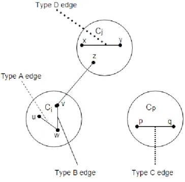
7 Types of intra edge additions-Cj is a neghboring community of node v, butCp is not. . . 31

8 Types of inter edge additions . . . 37

9 Effective factors for edge formation (a)Homophily (b)Triadic closure (c) Cyclic closure . . . 50

10 Football network edge distribution . . . 66

11 Email network edge distribution . . . 66

12 Facebook network edge distribution. . . 67

13 PGP network edge distribution . . . 67

14 Condmat network edge distribution. . . 68

15 DBLP network edge distribution . . . 68

16 Livejournal network edge distribution . . . 69

17 Difference in modularity with DSLM and without DSLM for Football n/w 70 18 Difference in modularity with DSLM and without DSLM for Email n/w . 70 19 Difference in modularity with DSLM and without DSLM for Facebook n/w 71 20 Difference in modularity with DSLM and without DSLM for PGP n/w . . 71

21 Difference in modularity with DSLM and without DSLM for Condmat n/w . . . 71

22 Difference in modularity with DSLM and without DSLM for DBLP n/w . 72 23 Difference in modularity with DSLM and without DSLM for Livejournal n/w . . . 72

25 Percentage of nodes crossing thresholds per phase for Email n/w . . . 81

26 Percentage of nodes crossing thresholds per phase for Facebook n/w . . . 81

27 Percentage of nodes crossing thresholds per phase for PGP n/w . . . 82

28 Percentage of nodes crossing thresholds per phase for Condmat n/w . . . 82

29 Percentage of nodes crossing thresholds per phase for DBLP n/w . . . 82

30 Percentage of nodes crossing thresholds per phase for Livejournal n/w . . 83

31 Modularity Analysis for Football Network for different edge addition models 86 32 Modularity Analysis for Email Network for different edge addition models 87 33 Modularity Analysis for Facebook Network for different edge addition models . . . 88

34 Modularity Analysis for PGP Network for different edge addition models 89 35 Modularity Analysis for Condmat Network for different edge addition models . . . 90

36 Modularity Analysis for DBLP Network for different edge addition models 91 37 Modularity Analysis for Livejournal Network for different edge addition models . . . 92

38 Time Analysis for Football network with different models . . . 93

39 Time Analysis for Email network with different models. . . 94

40 Time Analysis for Facebook network with different models . . . 95

41 Time Analysis for PGP network with different models . . . 96

42 Time Analysis for Condmat network with different models . . . 97

43 Time Analysis for DBLP network with different models . . . 98

List of Tables

1 Propositions for different types of intra edge addition . . . 31 2 Propositions for different types of inter edge addition . . . 38

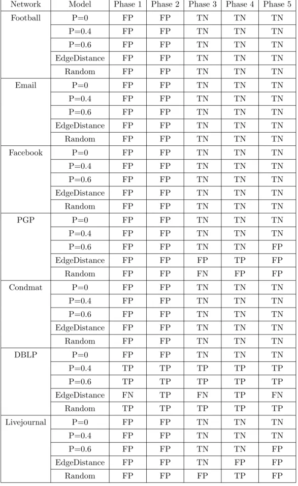
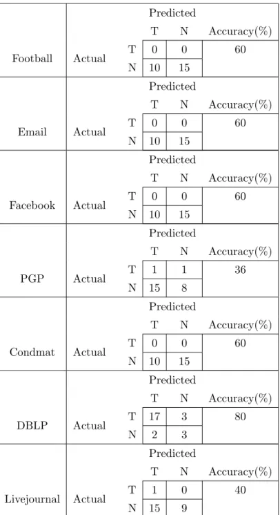
3 Characteristics of benchmark networks . . . 63 4 Edge distribution analysis over modularity for EdgeDistance model . . . . 65 5 Edge distribution analysis over modularity for Random model . . . 65 6 Ideal phases to update community structure . . . 73 7 Modularity-Change-Rate algorithm results . . . 76 8 Modularity-Change-Rate algorithm false positives and false negatives. . . 77 9 Confusion Matrix and Accuracy for Modularity-Change-Rate algorithm . 78 10 Deciding parameterα . . . 79 11 Values of M axP ercentCrossingfor different phases . . . 80 12 Edge-Distribution-Analysis algorithm false positives and false negatives . 84 13 Confusion Matrix and Accuracy for Edge-Distribution-Analysis algorithm 85

List of Algorithms

1 LocalMovingHeuristic(G) . . . 16

2 LouvainAlgorithm(G) . . . 18

3 CreateReducedNetwork(G, C) . . . 18

4 SLMAlgorithm(G) . . . 23

5 Iterative Variant for algorithms(G) . . . 25

6 ThresholdPercentage(Gj, Gj−1, M axP ercentCrossing) . . . 43

7 GenerateThresholds(Gj, Gj−1.cluster). . . 44

8 GenerateEdgeDistribution(Gj, Gj−1) . . . 45

9 DeltaModDslm(δm, Gj, P0) . . . 47

10 PhaseCalculation(δm, Gj, Gj−1, Gj−2, P0) . . . 47

11 RandomModel(Gj, percentageOf Edges). . . 51

12 EdgeDistance(Gj, percentageOf Edges) . . . 54

13 GeometricProbability(Gj, p, percentageOf Edges) . . . 57

14 AddIntraEdges(nIntraEdges, Gj, G0) . . . 58

Abbreviations

SLM SmartLocalMoving

DSLM Dynamic SmartLocalMoving LHM LocalMovingHeuristic EDA EdgeDistributionAnalysis MCR Modularity ChangeRate

Chapter 1

Introduction

Graphs have become remarkably useful to represent a wide range of systems of interest to scientists, engineers, and social scientists. Some examples are biological networks, telecommunication networks, Internet, world wide web, social networks, citation net-works and collaboration netnet-works. Social network analysis started in 1930 [19] and has become an important area of research in computer science. A social network is defined as a set of nodes connected by edges. Nodes could represent people, molecules, comput-ers or routcomput-ers and edges represent the connections between nodes. For example, in an email network, nodes represent a set of people in an organization, and an edge between nodes aand y indicates that there was an email exchange between x and y in a given time period. Advances in technology have made possible the collection of data on social networks that contain millions of nodes and billions of edges. The ever growing nature of such networks demands new methods to understand the hidden information from their structure.

One promising approach consists of decomposing the networks into sub-units or

communities, which are sets of highly inter-connected nodes [9], [20]. The problem of community detection has been studied extensively for static networks. However, most social networks are not static in nature. Many social networks evolve rapidly in terms of size over time. Nodes may join or leave social networks. Even the nodes that stay, may lose connections or create new connections. In popular online social networks like Twitter, Facebook, Livejournal, within 24 hours, millions of users update their connections. Such networks may be termed dynamic social networks. For large networks with millions of nodes and billions of edges, some thousands of edge additions or deletions might seem insignificant, but over time they change the structure of the network. In particular, communities in the network may evolve and change as a result

of edge additions or deletions. This change in community structure raises the need of re-identification of communities in the network [3]. In this thesis, we study the problem of community (re)-identification in dynamic networks. We call this the problem of dynamic community detection.

1.1

Community Detection

How do we define communities in a social network? A generally accepted, though somewhat vague, definition is that a communities are groups of nodes that have denser connections within the group than outside the group. We discuss different defintions of a community in the literature in Chapter 2. A classic example of social network that has been studied in this context is Zachary’s karate club network [52]. This network contains 34 nodes and 78 edges. The nodes of this network represent the members of karate club and the edges connect the people who had interactions outside the club. This network was observed for a period of three years. During this period, the president of the club and the instructor had a conflict which led to the breakup of the club into two separate groups, supporting the instructor and the president. A key question of interest is: Would it have been possible to predict this separation by simply examining the structure of the network? From Figure 1, we can easily distinguish two groups of nodes that have a lot of connections within the groups and few between the two groups. The aim of community detection algorithms is to identify such communities.

For large networks, efficient algorithms for community detection become very im-portant as it is impossible to visualize networks of millions of nodes. Community de-tection has a lot of applications in real networks. An important application is for rec-ommendation systems. It makes sense to make similar recrec-ommendations to a group of people who are in the same community and possess similar interests [45]. Another exam-ple is in research, the communities obtained from citation and co-authorship networks like DBLP and Condmat can be used to develop new methods and theories and can help to understand research patterns. In [17], the authors have tried to detect criminal ac-tivities in criminal networks using clustering algorithms. Traditional methods focus on the movement of an individual but here the authors claim that one should use commu-nities to detect these events. Community detection is also used for refactoring software packages in complex software networks [37]1 _{There are a lot of applications in biological}

networks, but one of the most significant is a community-based lung cancer detection approach which focuses on high risk patients [7]. In a protein-protein interaction (PPI) networks, communities correspond to functional groups, i.e to proteins having the same

1

Refactoring code means restructuring the code without changing its external behavior. Such refac-toring improves code readability and reduces complexity.

Figure 1: Zachary’s karate club network [4]

or similar functions, which are expected to be involved in the same processes. Some communities in these networks are related to cancer and metastasis, hence, detecting these communities in PPI networks could be very important [18]. Community detection can also be helpful in solving influence maximization or viral marketing problems.

1.2

Dynamic Networks

Social networks may be classified as static or dynamic. Static networks do not change or evolve over time; in dynamic networks nodes may come and go, and edges might be added or deleted. In simple terms, the network topology changes over time. Social network researchers may seem to perceive the world as static but dynamic networks are present everywhere. Fifty four years ago, Wilbert Moore said [31] that ”social sciences tended to neglect the way the limits and flows of time intersect the persistent and changeful qualities of human enterprises.” This observation was based on the dominance of static models to study social networks. He further stated that ”all analytical sciences tend to perfect their descriptions of elements and observations of combinations before they develop the capacity to observe orderly transformations in the course of time.” Till this date, static models are dominant in social network analysis.

A dynamic network is modeled as a sequence of graphsG0, G1, ..., Gn, whereGj =

(Vj, Ej) denotes the graph at snapshot j, which consists of Vj nodes and Ej edges

[43]. The example of Zachary’s karate club network is useful to be reconsidered here. We run Louvain’s [9] community detection algorithm on networkG0 which leads to four

communities which are represented by four different colors shown in Figure2.(a). Figure 2.(b) shows the next snapshot G1 of the graph in which we have added two new nodes

(node 35 and node 36) and 3 new edges from these nodes. Due to the change in network dynamics there is a need to re-run the community detection algorithm. The results of running community detection on graph G1 are shown in Figure 2.(c). From this, we

can observe that some of the communities are merged or split and new communities are created.

Figure 2: (a) Zachary’s karate club original network (b) Zachary’s karate club network

after addition of new nodes and edges (c) Result of the Louvain algorithm on Zachary’s

1.3

Problem Statement

In this thesis, we study the problem of community detection in dynamic networks. We as-sume we are given a dynamic evolving network, represented by snapshotsG0, G1, ..., Gn,

whereGj = (Vj, Ej) denotes the graph at snapshotj, which contains|Vj|nodes and|Ej|

edges. We assume that the only change to the network between the snapshots is the addition of new edges. We aim to have up-to-date and accurate community information for all snapshots. An obvious algorithm is simply to run a static community detection algorithm for every Gj. However this would be prohibitively expensive in general, and

completely infeasible for large networks. In addition, community structure may not change significantly between snapshots.

How many edges need to be added to the network until the community structure changes? Are some kinds of edges likelier to change community structure than others? Are some nodes likelier to switch communities than others? How do we model the evolution of communities? We aim to get a better understanding of these questions in this thesis. Our final goal is to find algorithms to decide in every snapshot, knowing only which edges have been added to the network, whether or not the community structure is likely to have changed, necessitating the execution of a static community detection algorithm, to update the community structure.

1.4

Thesis Contribution

The contributions of this thesis are listed below:

• We classify edges into different categories and compute the minimum (threshold) number of different types of edges that would need to be added to a network before its community structure would change.

• We give several models for the addition of new edges to a social network.

• We give two new algorithms: the Edge-Distribution-Analysis algorithm , and the Modularity-Change-Rate algorithm to solve the problem of identifying the snap-shotsGi in which to run a static community detection algorithm.

• We implement and run our algorithms on seven different benchmark social net-works, and analyze the results.

• Our experiments show that both our algorithms do a good job at identifying snap-shots in which to update the community structure. Compared to an approach

of updating community structure after a fixed number of edge additions, our al-gorithms obtain large savings in computation effort, while ensuring comparable quality of community structure.

1.5

Thesis Outline

Chapter 2 presents a literature review on community detection topics. First, we briefly explain the problem of community detection. Then we present different existing solutions for the problem. Chapter 3 presents our two new algorithms to solve the problem of dynamic community detection. Chapter 4 conducts a detailed study on generating evolving networks. Chapter 5 presents a comprehensive study of the performance of the proposed algorithms in the previous chapters. The final chapter concludes our thesis and gives some leads for future work.

Chapter 2

Related Work

In this chapter, we give a literature review on community detection. We start by at-tempting to define a community in Section 2.1. In Section 2.2, we study a few community detection techniques discussed within the literature. In Section 2.3, the literature on the Louvain algorithm and its variants have been reviewed. Section 2.4 extends the concept of community detection for evolving networks and details a few important algorithms from the literature. Finally, the limitations of existing algorithms have been outlined in Section 2.5.

2.1

What is a community?

In this section, we give the definition of community detection in depth and study some of the fundamental concepts of graph clustering. Afterwards, a brief explanation of the computation time for community detection is considered. There are many definitions of community detection. No definition is universally acclaimed. Often, the definition is based on the type of system under consideration or application dependent. After a careful review of these definitions, it can be concluded that communities are the subgraphs in which nodes are densely connected to each other when compared to the rest of the network. There are two types of community definitions; local and global. Local definitions focus on the subgraph under study but neglect the rest of the graph. On the other hand, in the case of global definitions, communities are defined with respect to the graph as a whole.

2.1.1 Local Definition

In social networks, a community often means a group whose participants are all friends with each other. In graph theory, such a group is termed as a clique in which every two distinct nodes are adjacent. This is a rather strict definition of community. According to this definition, if a single pair of nodes is not connected to other nodes in the network, it can be termed a community. Also a subgraph in which all but one pair of nodes is connected would not qualify as a community. Another important limitation of this definition comes about if we want to understand the hierarchical roles of nodes within the community. Using the definition of community as a clique, it is simply not possible.

One can always relax the notion of clique and define an n-clique. An n-clique is a maximal subgraph for which the distance between any pair of nodes does not exceed

n. There are problems associated with this definition as well which are stated in [18]. There are some definitions available that are based on the similarity of the nodes. Each node ends up in a community whose nodes are most similar to it. This similarity can be a local or global property of the network. For example it can be geographical distance between the two nodes, the degree of the nodes etc. Therefore, two nodes who are not connected to each other by a short path might appear in the same community. [16] and [18] provide some number of suitable local definitions, however, in this work, our focus is on global definitions.

2.1.2 Global Definition

In contrast to local definitions, in a global definition of community, we specify not only the relationship between nodes within the community, but also their relationship to nodes outside the community. A community is defined as a subgraph in which nodes are densely connected to each other and sparsely to the rest of the network. Within such a context, a global property of the graph is used in an algorithm which delivers communities. A key idea in the literature is that if a network has community structure, it is different from a random graph. Several definitions [18] draw on this notion. The random graph defined by [15], will not have community structure. As any two nodes of the graph have the same probability of being connected to each other, as a result, there will not be any special group or community. In the literature, the null model is defined as a random graph which matches the given graph in some of its structural properties. This null model is used as a comparison tool in order to find out whether the original graph exhibits community structure or not. The most famous proposed null model by [34] rewires the edges randomly by keeping the degree of the node the same as it was in the original graph. This new random graph is used as the null model.

This null model is the basic concept behind the global parameter modularity. There are a lot of definitions of modularity based on different null models. According to [34], a subgraph is a community only if the total number of internal edges in the subgraph are greater than the expected total number of edges that are inside the same subgraph of the null model. Modularity also acts as a quality function which maps any partition of the graph to a numerical value. Then the communities can be said to be the partition that maximizes this value. Since we adopt this approach in our thesis, we describe it in detail in the next section.

2.1.3 Quality function: Modularity

Modularity is a function that evaluates the quality of a given partition of nodes in a graph as good communities. It is based on evaluating how much the graph, and the given partition differ from null model.

Consider a graphG= (V, E) and let|V|=nand |E|=m. Suppose we are given a community structure e for the graph where e = C1, C2, ..Ck is a partition of V into

communities. Defined(v) to be the degree of nodev. Let Abe the adjacency matrix for

G where Avw = 1 means there is an edge from node v to node w and Avw = 0 means there is no edge from node v to nodew.

To obtain a null model, the following procedure is described in [34]. For every edge in the graph, we cut it in a half so we have twostubs. The total number of stubs is 2m. We now reattach the stubs at random to obtain a null graph G0. If (v, w) ∈ e, the probability thatv and w are connected inG0 is

d(v)d(w) 2m

Therefore, the difference between the actual number of edges and the expected number of edges between v andw is

Avw−d(v)d(w) 2m

The modularity of the partitioneis now defined to be the summation of the difference over all edges within communities [32]. In particular:

Q= 1 2m X vw Avw−d(v)d(w) 2m δ(cv, cw) (2.1)

wherecv denotes the community to which nodev belongs and δ(i, j) = 1 ifi=j and 0

that, they define two variables which are: ei,j = 1 2m X vw Avwδ(cv, i)δ(cw, j) (2.2)

ei,j denotes the fraction of edges connecting nodes in community ci and cj. Further let,

ai = 1 2m X v d(v)δ(cv, i) (2.3)

ai denotes the fraction of edges who have one endpoint in communityi. It was shown in [13] that

Q=X

i

(eii−a2_i) (2.4)

Notice that modularity can be seen in two different ways:

• Given a graphGand two different community structures e1 ande2 forG, the one

that has a higher associated modularity value reflects tighter connections within communities. Thus modularity is a way of assessing different communities struc-tures for a graph.

• Given two graphs G1 and G2 with similar structural characteristics (number of

nodes, edges, and node degrees), and best possible community structure for them, the graph that has a higher modularity value can be said to have tighter commu-nities. Thus modularity is a way of assessing how strong the community structure is in a graph.

It can be shown that the value of modularity resides in between [−1

2,1). In [32], the definition of this modularity is extended for weighted networks, but within this thesis, we focus on unweighted networks.

2.1.4 Maximizing a modularity is NP-hard

Theorem [3] of [12] states that maximizing modularity is strongly NP-complete. The proof is based on reduction from the 3-Partition decision problem which can be stated as follows: Given 3k positive integer numbersa1, ..a3k such that the sumP3i=1k ai =kb

and b₄ < ai < ₂b for an integer b and for all i = 1, ..,3k, is there a partition of these numbers into k sets, such that the numbers in each set sum up to b. Therefore, they suggest the use of heuristics for maximizing modularity.

2.2

Techniques of Community Detection

There is a variety of algorithms for community detection that are based on different definitions and the size of the networks. For every definition, there is at least one algorithm in literature. In [18], the authors perform an in-depth review of the relevant literature, detailing more than 20 algorithms for community detection. According to [38] and [18], community detection methods are divided into different classes. In this section, we describe several existing strategies from these classes namely traditional, divisive, modularity based and some of the other methods.

2.2.1 Traditional algorithms

Traditional algorithms are further categorized into following four classes:

• Graph partitioning: The problem of community detection has been studied since the 19th century. Earlier version of this problem resembled the problem of graph partitioning. The problem of graph partitioning consists of dividing the graph into fixed groups of a predefined size such that edges between groups are minimized. This problem is quite well-known due to its applications in parallel computing and circuit partitioning. Some of the popular approaches were Kernighan-Lin

[23], spectral bisection [42] etc. Such algorithms are not good for community detection as they require the knowledge of the number of communities and the size of communities in advance to run the algorithm. In reality, one should find these values after running a community detection algorithm.

• Hierarchical clustering: Quite often, social network contain hierarchical structure. In such cases, one can use hierarchical clustering techniques such as:

1. Agglomerative algorithms: Nodes are merged iteratively based on the some similarity measure.

2. Divisive algorithms: Supernodes are split into nodes by removing edges which connects the dissimilar nodes. This creates structure similar to a dendrogram. From Figure 3, we can observe the hierarchical structure of nodes.

• Partitional clustering: Similar to graph partitioning, within partitional clustering, one should know in advance the number of clusters for given graph. The main goal is to divide the nodes into k clusters by maximizing or minimizing some measure such as the shortest distance, similarity etc. Famous approaches include

Figure 3: Hierarchical dendrogram for Zachary’s karate network club [35]

of minimum k-clustering is the diameter of the cluster. For the largest cluster, diameter should be as small as possible. The idea is to keep the clusters compact. In case of an k-clustering sum, diameter is replaced by average distance for all pairs of points of a cluster. This approach also faces the same problems as graph partitioning.

• Spectral clustering: This type of clustering includes all the methods which use eigenvectors of matrices based on similarity to group the nodes. for example, algorithms given in [8] and [36].

2.2.2 Divisive algoritms

The Girvan and Newman algorithm [33] is a benchmark algorithm. It started a new era of community detection. Betweenness of an edge is defined as the total number of shortest paths for all the pairs of nodes that use the edge [18]. The steps of the algorithm are as follows:

1. Compute the edge betweenness centrality for every edge.

2. Remove the one with largest centrality; choose randomly in case of a tie.

3. Recalculate centralities for current version of graph.

The authors have used this algorithm for a network of jazz musicians and divided them into communities that are based on their collaboration efforts with each other. The worst case complexity of an algorithm is O(n3) which made it impossible to extend the algorithm for networks with size greater than 10000. Authors have used the edge betweenness as centrality measure in later versions to obtain better results. There are many other algorithms which use different centrality measures such as node centrality based on loops, similar to the clustering coefficient by [39].

2.2.3 Modularity based algorithms

The modularity function is by far the most used and most significant quality function. Girvan and Newman used it as a stopping criteria for their divisive algorithm. Since then a variety of algorithms have been proposed which focus on modularity optimization. Spectral clustering, divisive techniques or simulated annealing [22] have been used for modularity optimization. In 2008, a new heuristic for modularity optimization called the Louvain method was introduced by Blondel [9]. Today this is the fastest algorithm, for large networks. The modularity obtained by this algorithm is not the best as compared to other algorithms provided in literature. However, considering the time-modularity trade off, it gives exceptional results. This algorithm is further extended by Noack and Rotta [41] to improve the proposed heuristic. Their algorithm is known asThe Louvain algorithm with multilevel refinement. In [30], they exploit the measure of edge centrality for modularity optimization. Their approach is called Generalized Louvain method. In 2013, Waltman & Ludo [47] introduced a newer algorithm called SLM based on [9]. We have used the aforementioned algorithms in our thesis. A detailed discussion of these algorithms is provided within Section 2.3. The limitations of modularity based algorithms are discussed at the end of the chapter.

2.2.4 Other methods

In [18], the authors have published a book explaining all the community detection algo-rithms present till 2010. Apart from the ones that we have mentioned, there are other algorithms based on spin models, conformational space annealing [26], random walks and synchronization. Also, there is separate section for methods based on statistical infer-ence. Some of these algorithms address different aspects of community detection which are not our focus. For example, our thesis does not focus on overlapping communities but there are few algorithms which allow for this.

2.3

Communities in large networks: The Louvain

Algo-rithm and its variants

As per our discussion in Subsection 2.2.3, the Louvain algorithm is a benchmark algo-rithm for community detection in large networks. In this section, we give a detailed explanation of this algorithm and its variants. A fundamental part of this algorithm is the so-called local moving heuristic. The concept behind the local moving heuristic is to move the nodes repeatedly from one community to another community as long as there is gain in modularity. The gain in modularity by moving an isolated node v into communityCi is calculated as follows:

∆Q= Ei+ 2∗di(v) 2m − D(i) +d(v) 2m 2 − Ei 2m − D(i) 2m 2 − d(v) 2m 2 (2.5)

whered(v) denotes the degree of the node,mdenote the total number of edges,D(i) the sum of the degrees of the nodes in communityCi,di(v) represents the number of edges from nodevto other nodes in communityCi and finally,Ei denotes the total number of

edges for which both the endpoints are in communityCi. The first part of Equation2.5 represents the modularity obtained by moving node v into community Ci. The second

part of shows the modularity obtained when the node v is an isolated node. Equation 2.5uses the simplified Equation 2.4for modularity.

2.3.1 Local moving heuristic

In this section, we describe the Local Moving Heuristic. The local moving heuristic has been used in [6], [9], [41], [29], [47] etc. Initially, every node is in its own commu-nity. Next, we take an arbitrary node and see if including it in any of its neighboring communities increases the modularity. We check all neighboring communities and find the best community that v can move to. We repeatedly do this until no nodes switch communities. The pseudocode is given in Algorithm1.

In line 1, we shuffle the nodes randomly. According to [9], the order in which nodes are chosen might affect the computation time. The do-while loop of lines 4-18 iterates as long as total number of stable nodes are less than total number of nodes. In line 5, we choose the node for which we will calculate the best possible community. In for loop of lines 6-11, we compute the gain in modularity by moving singleton nodevto adjacent community c using Equation 2.5. Here adjacent community means that node

v has direct edge to any of the nodes in communityc. If the node v is already assigned to some community then, before the next step, it is removed from that community & similar expression to Equation 2.5 is used to calculate this change in modularity. In

Algorithm 1 LocalMovingHeuristic(G) 1: V =Shuffle(V) 2: j= 0 3: update=f alse 4: do 5: v=V[j]

6: for each c∈G.Adj[cv]do

7: computeδQ for nodev and community cusing Equation 2.5 8: if δQ≥maxQ then

9: maxQ=δQ

10: bestCluster =c

11: end if

12: if bestCluster==cv then

13: nStableN odes←nStableN odes+ 1

14: else

15: nStableN odes= 1

16: update=true

17: end if

18: whilenStableN odes < V

19: return update

practice, one considers this change and the gain obtained by moving node to community

c. Lines 8-11 keeps track of the maximum gain in modularity and best community assignment for node v. Lines 12-13 checks whether the previous assignment of node v

is the still the best. In such case, we increase the total number of stable nodes by 1. Otherwise, we initialize the update to true and the number of stable nodes to 1. This means that algorithm might consider the same nodes many times. This procedure keeps running until one does find the best possible assignment for every node.

Figure 4 shows an example of running local moving heuristic to the Karate club network [52] that has 34 nodes and 78 edges. After running the Local Moving Heuristic,

we observe that there are six communities. The green and red communities contain most of the nodes.

2.3.2 Louvain Algorithm

The Louvain algorithm adds an additional level to the Local Moving Heuristic(LMH). Essentially, it takes the communities given by LMH and creates a reduced graph in which nodes correspond to the previously found communities. It then recursively finds communities in this reduced graph. The recursive calls stop when every node in the reduced graph stays in a singleton community when the LMH is applied. Finally, the nodes of the reduced graph are used to assign communities in the original graph. The pseudocode of the Louvain algorithm is given in Algorithm2.

The Louvain algorithm works as follows: Lines 1-3 checks whether the graph has more than one nodes and returns false in such cases. In line 4, we read the network and assign every node to an individual singleton community. In line 5, we run the LocalMovingHeuristicand pass graphGas parameter. The aim of the local moving heuristic is to achieve the highest possible gain in modularity for every node. Lines 6-14 are executed only if the total number of communities are less than the total number of nodes. In line 7, we create reduced network with less number of nodes based on the resulting communities that are obtained from local moving heuristic. This is the first phase of an algorithm. From line 8, we can observe that the Louvain algorithm is written in recursive fashion. The reduced network is passed as a new instance for the Louvain algorithm. Lines 9-13 are executed only if through running the Louvain algorithm we have obtained positive gain in modularity. The for loop of lines 11-12 assigns the new communities to nodes based on the output of every phase. This is the merging step of the Louvain algorithm. After this we explain the construction of the reduced network in depth.

We give an example of running the Louvain algorithm on the Karate club network [52] which has 34 nodes and 78 edges. Figure 4 illustrates an example of running lo-cal moving heuristic, we observe that there are six communities. Algorithm3 gives the pseudocode for the construction of the reduced network. In line 1, we create the nodes of the reduced network. Every community obtained after running the local moving heuris-tic will be considered as a node in reduced network. V_v0 denotes the new supernode in the reduced network which containd node v. In the outer for loop, each community is considered one by one. For all the nodes which belongs to community under consider-ation, we check for every edge whose one of the endpoint is nodev. The weight of the edges between two supernodes denote the sum of all the links between the nodes in the

Algorithm 2 LouvainAlgorithm(G) 1: if G.V == 1 then 2: return f alse 3: end if 4: _ReadInput(G) 5: update=LocalMovingHeuristic(G) 6: if |G.C|<|G.V|then 7: G0 =CreateReducedNetwork(G, C)

8: newU pdate= LouvainAlgorithm(G 0

)

9: if (newU pdate) then 10: update=true 11: forv= 1 toV do 12: C[v] =C[C0[v]] 13: end if 14: end if 15: return update Algorithm 3 CreateReducedNetwork(G, C) 1: LetV0 = 1,2, ..C 2: fori= 0 toC do 3: for each v∈Ci do

4: foreach edge (v, w)∈E do

5: e(V_v0, V_w0)←e(V_v0, V_w0) + 1

Figure 4: Result of applying local moving heuristic to karate club network [47].

corresponding two communities. Edges between the nodes of the same community are treated as self loops for this supernode. This is achieved by line 5. In line 6, we return the reduced network. Figure 5 gives the results of applying the Louvain algorithm for the karate network. Figure 5.a represents the reduced network of six communities after running local moving heuristic. We have not shown the self loops in it but they do exist. After running local moving heuristic again on this reduced network we get Figure 5.b. We can notice that nodesbandcnow belong to same community. Similarly nodeseand

f also now belong to same community. The new reduced network consists of four nodes. In the next phase, on running local moving heuristic, the change in modularity is not positive. We use these nodes from reduced network to assign communities in original graph. Hence, the final community structure is shown in Figure 5.c.

2.3.3 Louvain Algorithm with Multilevel Refinement

An extension of the Louvain algorithm was proposed in [41] in 2011. After running the Louvain algorithm we observed that no further gain in modularity is possible by merging communities. Actually, this is the stopping phase for the algorithm, in simple words, we find the locally optimal solution with respect to merging of the communities. In the Louvain algorithm, once the nodes are merged into supernode, individual nodes from the supernode cannot be moved to other communities. However, the final com-munity structure obtained by Louvain, can further be improved by allowing individual movements for the nodes.

Figure 5: Result of applying the Louvain algorithm to the karate club network[47].

(a) Reduced network before applying LMH (b) Reduced network after applying the LMH (c) Final solution in the original network

The Louvain algorithm with multilevel refinement [41] improves the solution of the Louvain algorithm so that it becomes locally optimal with respect to individual node movements. In order to perform this, the authors run the local moving heuristic twice. First, to obtain the initial community structure for the reduced network, and after that, they run local moving heuristic again to allow individual node movements. This procedure is applied to each level of an algorithm. Hence, it is called as multilevel refinement. This algorithm gives a significant improvement over the Louvain algorithm in terms of modularity, but the running time was also increased.

2.3.4 SLM Algorithm

Another extension of the Louvain algorithm was proposed by [47]. Their solution is also locally optimal with respect to community merging and individual node movements. In

addition to this, this solution checks for further improvements in modularity by splitting up communities and moving a set of nodes from one community to other communities. The idea of the algorithm can be summarized in 3 steps:

1. Run the Local Moving Heuristic on graphGto obtain an initial community struc-turee=C1, C2, ..Ck

2. Run separately the LMH on communities Ci to break (potentially) Ci into sub-communitiesCi,1, Ci,2, ..Ci,j

3. Create a reduced graph withCi,1, Ci,2 etc. as nodes (for alli), but use the original

community structure e, and recursively call the algorithm on the reduced graph and community structure.

Algorithm 4gives the pseudocode of the SLM algorithm.

Lines 1-3 check whether the graph contains a single node; in such a case, it returns false. In line 4, we read the graph and assign every node to individual community. In line 5, we run local moving heuristic as in to the Louvain algorithm. Lines 6-17 are executed only if number of communities obtained from local moving heuristic is less than total number of nodes. From line 7, authors take different approach. Instead of creating the reduced network right away, they construct a copy of subnetwork for every community present in the current community structure. This copy will contain the nodes belonging to particular community of interest of the original network. For loop of lines 9-13, runs local moving heuristic for each of the subnetwork in order to identify the communities inside the subnetwork. Similar to original procedure, every node of the subnetwork is assigned to individual community and then local moving heuristic is ran on it. The result after running the local moving heuristic on subnetwork might be a single big community including all the nodes of subnetwork or it might consists of multiple communities including some of the nodes from subnetwork. In line 13, nClusters will contain total number of communities obtained by running local moving heuristic on all the subnetworks. In line 14, one creates a reduced network where each node of reduced network represents a community obtained from one of the subnetworks. Nodes corresponding to communities in the same network are assigned to same community in the reduced network. Therefore, for every subnetwork one gets single community in the reduced network. This is achieved in lines 12-13. Once the reduced network is created, we recursively call SLM on this network.

To illustrate the SLM algorithm, the karate club network is reconsidered. Figure 6(a) shows the six communities which are generated after running local moving heuristic.

Each community is represented by different colour. For each community new subnet-work is created. On every subnetsubnet-work, local moving heuristic is applied. For green, blue, purple and yellow it results into all nodes being assigned to a single community. In the case of red and orange, subnetworks are split into two communities. This is represented by different shapes such as the squares and circles. Figure 6(b) shows the reduced network that is obtained. In this reduced network, we have 8 nodes. Each node represent a community in subnetwork. Nodes corresponding with communities in the same subnetwork are assigned to the same community initially. The result of applying local moving heuristic on it is shown in6(c). We observe that nodesA1 andA2 remain in the same community but nodes C1 and C2 now belong to different communities. Afterwards, we again create subnetworks and run the local moving heuristic for every subnetwork. We do not show the result of this, since it turns out that the community structure shown in Figure 6(c) cannot be improved further.

2.3.5 Iterative variant of these algorithms

The authors of the [47], introduced an approach that aims to improve all of the stated algorithms above. The basic idea of this approach is to run in iterative fashion, where the output of previous iteration will be the starting community assignment for the next iteration. In any of the algorithms like Louvain, Multilevel Louvain or SLM, they start by assigning each node to an individual community. This approach will do the same, but after the first iteration, the result of the first iteration is given to second iteration. Therefore, for the second iteration, one does not start with every node as singleton community. Instead one starts with the community structure of the first iteration. The procedure is repeated for the number of iterations specified or one can stop the algorithm when an additional iteration is not giving a gain in the modularity. Also in the original paper of Louvain, it is mentioned that the order in which nodes are chosen is important, hence, certain number of random starts are provided to obtain the best result. Algorithm 5 explains the procedure. In line 6, by runAlgorithmwe mean that you can run Louvain, Multilevel Louvain or SLM.

Algorithm 4 SLMAlgorithm(G) 1: if G.V == 1 then 2: return f alse 3: end if 4: _ReadInput(G) 5: update=LocalMovingHeuristic(G) 6: if G.C < G.V then 7: G=CreateSubNetworks(G, C) 8: nClusters= 0

9: for each edge subnetworkGi∈Gdo

10: _{LocalMovingHeuristic}(Gi) 11: forj= 0 to Vi do 12: C[j] =nClusters+Ci[j] 13: nClusters←nClusters+Ci 14: G0 =CreateReducedNetwork(G, C) 15: update=SLMAlgorithm(G0) 16: for v= 1 toV do 17: C[v] =C[C0[v]] 18: end if 19: return update

Figure 6: Result of applying the SLM algorithm to karate club network[47]. (a)LMH is applied on six subnetworks. Nodes in the subnetwork are displayed using either square or circle. (b) Reduced network before applying the LMH. (c) Reduced network

Algorithm 5 Iterative Variant for algorithms(G) 1: fori= 0 torandomStarts do 2: update=true 3: iteration= 0 4: do 5: IntializeCommunities(C) 6: update=runAlgorithm(G)

7: modularity=CalculateM odularity(G, C)

8: iteration←iteration+ 1

9: while iteration < nIterationsandupdate

10: if modularity≥maxM odularity then

11: maxM odularity=modularity

12: end if

2.4

Dynamic Community Detection for Evolving Networks

Dynamic community detection is still in its infancy. The reason for this is, as the problem is NP-hard, solving the problem of community detection for static graph is already difficult. Thus, most of the studies focus on the practically efficient static versions of this problem. In [18], it is mentioned that the main phenomena occuring in the lifetime of community are birth, growth, contraction, merger with other communities, split and death. In the literature, some of the studies like [44], [43], [10] have focused on predicting the evolution of networks and then they use that information for community detection. On the other hand some approaches like [3] focus on using the information from the previous snapshots and perform community detection based on it.

2.4.1 DSLM Algorithm

The authors of [3] have extended the SLM algorithm for dynamic community detection. The idea of the DSLM algorithm is summarized as follows:

1. Detect the new nodes which are added to the network and assign them as singleton communities.

2. Read the previous community structure for the given graph G and assign the current nodes to the communities based on it.

3. Run the SLM algorithm with this community structure as starting assignment.

Addition of edges, deletion of nodes and edges is handled by the SLM algorithm. This algorithm does very well in terms of running time as compared to running SLM from scratch on Gi. The main innovation in this algorithm is that rather than running SLM from scratch on each Gi, we use the community structure of Gi−1 that was derived

previously as a starting point for SLM. This is responsible for saving time.

The authors of DSLM do not indicate how often to run the algorithm. For example after the addition of how many nodes or edges should DSLM be run? In terms of modularity DSLM gives more or less the same result as SLM.

2.4.2 Community Evolution Prediction Algorithm

In [44], the authors have proposed a machine learning model to accurately predict the changes and transitions of the community based on structural and temporal properties.

Community transitions and events are considered as response variables. They have used features of communities such as density, clustering coefficient, number of nodes, cohesion, average closeness, average degree, variance closeness and variance degree which influence one of the response variables. Different snapshots of the networks are collected and analyzed. Next, they have used logistic regression and various classification functions to train the data and predict the community transitions. Their experiments show that defined features are non overlapping and community transitions and events are predicted accurately.

2.5

Limitations of existing algorithms

We have surveyed different definitions of communities and algorithms for community de-tection problem. First of all, the solutions given in the literature are heuristics hence, it is not possible to find the exact solution. Secondly, due to the plethora of application-based definitions, it is hard to use one particular algorithm for all the community detection problems. For example, the authors of [48], [50] have focused on finding overlapping communities, while according to the Louvain algorithm, one node cannot be part of two communities at the same time. In [5], the focus is on finding communities in bipartite graphs. The authors of [51] give an algorithm to find out 2-mode communities or hidden communities in which nodes might not have direct links to each other but they have links to other nodes in coordinate way. For example, a network of politicians where hidden community can be presidents of nations but in the network they might not be connected at all but their degree distributions are similar.

In this thesis, we will be focusing on modularity-based algorithms. As per [12], maximizing modularity is NP-hard. Also one of the major drawback for all the modu-larity based approach is the so-calledresolution limit[18]. Due to this, in large networks sometimes such algorithms fail to resolve small communities even when they are well defined. The reason behind this is that, in the null model, it is assumed that nodes can get connected to any of other nodes in the graph. This assumption is a little unreason-able as the horizon of the node is limited to a small network. As a result, the expected number of edges between the two groups is decreased. In some of the cases, a single edge between two small clusters might lead to their merging. In [46], the authors have cited algorithms which do not suffer from the problem of resolution limit.

Finally, there are not many promising algorithms for the problem of dynamic community detection for evolving networks. One of the most promising approaches is [44] but it also predicts transition of communities with accuracy varying from 60 % to

90 %. In the next chapter, we propose two algorithms for solving community detection for evolving networks.

Chapter 3

Two Algorithms for Dynamic

Community Detection

In this chapter, we propose two new algorithms for dynamic community detection. We assume that we are given a partition of a graph into communities and a set of new edges are subsequently added to the graph. Some existing approaches for dynamic community detection in evolving networks were described in the previous chapter. The analysis of dynamic communities is still in its infancy [18].

3.1

Notation and preliminaries

The following notations will be used throughout the chapter [43]. A dynamic evolving network is modeled as a sequence of graphsG0, G1, ..., Gn, whereGj = (Vj, Ej) denotes

the graph at snapshot j, which containsVj nodes andEj edges. LetGj.mod represent the modularity for the graph Gj. We start with the discussion of the number of edges

that need to be added to the graph in order for the community structure to change.

Fix a graphG= (V, E). The remaining discussion in this section pertains to any such graph G. Let C be a community structure for G obtained by running the SLM algorithm. 1

We use d(v) to denote the degree of node v, and di(v) to denote the number of edges from node v to other nodes in the community Ci. Furthermore, let D(i) be the

1

As per our discussion in Section2.1.4, finding maximum modularity isNP-hard. This community structure does not have maximum modularity.

sum of degrees of nodes in the community Ci, that is:

D(i) = X

v∈Ci

d(v)

Finally, letm represent the total number of edges in the graph.

The gain in the modularity by moving an isolated node v to community Ci is obtained from Equation 2.5.

δQ=di(v)− d(v)D(i)

2m (3.1)

Fact 1. Let G be a graph and let C be a community structure for G computed by SLM or DSLM [47],[3]. Then C is locally optimal in the sense that for every nodev∈Ci and Cj 6=Ci, we have:

di(v)−d(v)D(i)

2m > dj(v)−

d(v)D(j) 2m

Given a community structure C, and a node v ∈ Ci, we say v wants to switch communities if there exists a community Cj with j6=isuch that

dj(v)−

d(v)D(j)

2m > di(v)−

d(v)D(i) 2m

Also, communityCj will be aneighboring communityof nodev, if there is a direct edge between node v and any node in community Cj. Node v might want to switch commu-nities based on various factors like the addition of edges, deletion of edges, addition of new nodes or deletion of new nodes. In this thesis we will be focusing on the addition of edges. We can distinguish two types of edges. We call an edge an intra-edge if it connects two nodes in thesame community. We call an edge aninter-edge if it connects two nodes indifferent communities.

3.2

Effect of edge additions on community structure

In this section, we study the effect of edge additions on community structure. We study first the effect of adding intra-edges, then the effect of adding inter-edges.

The main question we seek to answer is : how many edges need to be added to the graph before the community structure is changed. We focus on a single node

v in a community Ci. How many and what kind of edge additions would cause v to switch communities? We study intra- and inter-edge additions separately in the next two sections.

3.2.1 Addition of intra community edges

In this section, our aim is to understand the effects of intra-edge additions on commu-nity structure C in the graph G. We would like to identify the maximum number of intra-community edges that can be added without affecting the community structure. Consider a node v in Ci. From v

0

s vantage point, intra-edges can be further classified into 4 types, as shown in Figure7.

Figure 7: Types of intra edge additions-Cjis a neghboring community of nodev, but

Cp is not.

We call an intra-edge a type A edge if it connects two nodes in Ci but it is not

incident on v itself. We call it a type B edge if it connects v to another node in Ci. We call it a type C edge if it connects two nodes in community Cp where Cp is not a

neighboring community of node v. An intra-edge is a type D edge if it connects two nodes in communityCj whereCj is a neighboring community of nodev. Our results for each type of intra edge addition are summarized in Table1.

Type of edge Proposition

A Lemma1

B Lemma1

C Lemma2

D Lemma3

Type A and B intra-edges

The following lemma considers the addition of type A and B intra-edges to the graph

G.

Lemma 1. LetG= (V, E)be an undirected graph, andCbe a locally optimal community structure forG. FixCi ∈ C and let v∈Ci be an arbitrary node. Let Cj be a neighboring community of node v with j 6=i. Then node v does not want to switch to community Cj, if at most κjv new type A and B intra-edges are added between nodes in Ci, where κjv is given by:

κj_v =j2m(di(v) − dj(v)) + d(v)(D(j) − D(i)) 2(dj(v) − di(v) + d(v))

k

and there is no other change to the graph.

Proof. Since C is a locally optimal community structure for G, observe that by Fact1, we have: di(v)− d(v)D(i) 2m ≥dj(v)− d(v)D(j) 2m

Now, suppose thatk ≤κjv new edges between nodes in Ci are added to G. First v is not the endpoint of any of the k newly added edges that is, all the new edges are Type A edges with respect to node v. Observe that d(v), di(v), dj(v), D(j) will remain

unchanged. However,D(i) andmare both incremented by 2kas a result of the addition of the knew intra edges.

For node v, we will compare the change in modularity if v switches to Cj. We only consider a neighboring community Cj since only D0(i) and m0 have changed. So,

v against communityCi andCj, we have:

k≤ 2m(di(v) − dj(v)) + d(v)(D(j) − D(i)) 2(dj(v) − di(v) + d(v))

=⇒2dj(v)k+ 2d(v)k−2di(v)k ≤ di(v)2m−d(v)D(i) +d(v)D(j)−2dj(v)m

=⇒2dj(v)m+ 2dj(v)k−d(v)D(j) ≤ di(v)2m+ 2di(v)k−d(v)D(i)−2d(v)k

Dividing by 2m+ 2kon both sides, we obtain:

2dj(v)m + 2dj(v)k − d(v)D(j) 2m + 2k ≤ di(v)2m + 2di(v)k − d(v)D(i) − 2d(v)k 2m + 2k =⇒dj(v)− d(v)D(j) 2m+ 2k ≤ di(v)− d(v)(D(i) + 2k) 2m+ 2k (3.2)

This implies that node v does not want to switch to community Cj. Next, we consider

the case when some of the newly added edges are incident to v, i.e type B intra-edges. We need the following technical claim.

Claim 1.

D(i)−D(j)−2m dj(v) − di(v) + d(v)

≤0

Proof. Observe that

di(v)≤d(v)

∴ d(v)−di(v) +dj(v)≥0 On the other hand,

D(i)≤2m

∴D(i)−D(j)−2m≤0 The claim follows.

Now, suppose we add k ≤ κjv new edges between pairs of nodes (u, w) where u ∈ Ci, w ∈Ci and u 6= w. Out of these k edges, let p be type B intra-edges, that is

v=u orv=w. We know that

k≤ 2m(di(v) − dj(v)) + d(v)(D(j) − D(i)) 2(dj(v) − di(v) + d(v))

After the addition ofk edges, we have:

d0_i(v) =di(v) +p, d0(v) =d(v) +p, D0(i) =D(i) + 2k, m0 = 2m+ 2k

D(j) remains the same. Observe that

2k≤ 2m(di(v) − dj(v) +d(v)(D(j) − D(i))) (dj(v) − di(v) + d(v)) =⇒2k+p D(i)−D(j)−2m dj(v) − di(v) + d(v) ≤ 2m(di(v) − dj(v)) + d(v)(D(j) − D(i)) (dj(v) − di(v) + d(v))

where the implication follows from Claim 1

Simplifying, we obtain:

2k(dj(v)−di(v) +d(v)) +p(D(i)−D(j)−2m)≤2m(di(v)−dj(v)) +d(v)(D(j)−D(i))

Dividing by 2m+ 2k on both sides, we obtain:

2mdj(v) + 2dj(v)k−d(v)D(j)−pD(j) 2m+ 2k ≤ 2mdi(v) + 2mp+ 2di(v)k 2m+ 2k +−d(v)D(i)−2d(v)k−pD(i) 2m+ 2k ≡dj(v)− (d(v) + p)D(j) 2m+ 2k ≤di(v) + p− (d(v) + p)(D(i) + 2k) 2m+ 2k (3.3)

Type C intra-edges

The next lemma considers the addition of type C intra-edges to the graph G.

Lemma 2. LetG= (V, E)be an undirected graph, andCbe a locally optimal community structure for G. Fix Ci ∈ C and let v∈Ci be an arbitrary node. Let S(v) be the set of all the neighboring communities of node v and Cj be a neighboring community and Cp is non-neighboring community. Then node v does not want to switch to community Cj, if we add at most αjv new type C intra-edges to community Cp where, Cj ∈ S(v), and αvj is given by:

αj_v = 2m(di(v) − dj(v)) + d(v)(D(j) − D(i)) 2(dj(v) − di(v))

and there is no other change to the graph.

Proof. Suppose we add k ≤ αvj new edges between pairs of nodes (u, w) where, u ∈ Cp, w∈Cp, and Cp ∈/ S(v). For the nodev∈Ci. Clearly,d(v), di(v), dj(v) will remain unchanged. Also, we have not added any edges to communities in S(v) henceD(i) and

D(j) will also remain unchanged.

In the new graph G0, when we will compare the change in modularity for an isolated node v against communityCi and Cj, we have:

k≤ 2m(di(v) − dj(v)) + d(v)(D(j) − D(i)) 2(dj(v) − di(v))

≡2(dj(v) − di(v)) ≤ 2di(v)m − d(v)D(i) − 2dj(v)m + d(v)D(j)

≡2dj(v)m + 2dj(v)k − d(v)D(j) ≤ 2di(v)m + 2di(v)k − d(v)D(i)

Dividing by 2m+ 2k on both sides, we get:

2dj(v)m + 2dj(v)k − d(v)D(j) (2m + 2k) ≤ 2di(v)m + 2di(v)k − d(v)D(i) (2m + 2k) ≡dj(v) − d(v)D(j) (2m + 2k) ≤ di(v) − d(v)D(i) (2m + 2k) (3.4)

According to Equation (3.4), community Ci is still the best option for node v between CiandCj, hence, there is no change in the community structure. So unless we add more

thanαjv edges, nodev will not switch its community toCj. Similarly, we can calculate αvj for all the neighboring communitiesCj ∈S(v).

Type D intra-edges

The following lemma considers the addition of type D intra-edges to the graph G.

Lemma 3. LetG= (V, E)be an undirected graph, andCbe a locally optimal community structure for G. Fix Ci ∈ C and let v∈Ci be an arbitrary node. Let S(v) be the set of all the neighboring communities of node v and Cj ∈S(v). Then node v does not want to switch to community Cj ∈S(v), if we add at most βvj new type D edges to community Cj where βjv is given by:

β_vj = 2m(di(v) − dj(v)) + d(v)(D(j) − D(i)) 2(dj(v) − di(v) − d(v))

and there is no other change to the graph.

Proof. Suppose we add k ≤ βvj new edges between pairs of nodes (u, w) where, u ∈ Cj, w∈Cj, andCj ∈S(v). For the nodev ∈Ci, we have not added any edges incident on it, therefore, d(v), di(v), dj(v) will remain unchanged. Also, we have not added any edges to community Ci, hence, D(i) will also remain unchanged. D(j) is incremented

by 2k.

In the new graph G0, when we compare the change in modularity for an isolated node v against communityCi and Cj, we have:

k≤ 2m(di(v) − dj(v)) + d(v)(D(j) − D(i)) 2(dj(v) − di(v) d(v))

≡2k(dj(v) − di(v) − d(v)) ≤ 2di(v)m − d(v)D(i) − 2dj(v)m + d(v)D(j)

≡2dj(v)m + 2dj(v)k − d(v)D(j) − 2kd(v) ≤ 2di(v)m + 2di(v)k − d(v)D(i)

Dividing by 2m+ 2k on both sides, we obtain :

2dj(v)m + 2dj(v)k − d(v)D(j) − 2kd(v) (2m + 2k) ≤ 2di(v)m + 2di(v)k − d(v)D(i) (2m + 2k) ≡dj(v) − d(v)(D(j) + 2k) (2m + 2k) ≤ di(v) − d(v)D(i) (2m + 2k) (3.5)

According to Equation (3.5), community Ci is still the best option for node v between

Ci and Cj, hence, there is no change in community structure. So unless we add more

thanβvj edges, nodev will not switch its community to Cj. Similarly, we can calculate βvj for all the neighboring communitiesCj ∈S(v).

3.2.2 Inter community edge addition

Our objective in this subsection is to analyze the impact of inter community edge addi-tions to community structureC in the graph G.

Figure 8: Types of inter edge additions

Consider nodev∈Ci. There are four types of inter edge additions from the point

of view of v, which are shown in Figure 8. We call an inter-edge a type A edge if it connects v to a node in any community except community Ci, Cj may or may not be

a neighboring community of v, but Cp and Cq are not neighboring communities. We call it a type B edge if it connects two nodes from communities Ci and Cj, where Cj

is neighboring community of node v. An inter-edge is a type C edge if it connects two nodes from communitiesCp and Cq whereCp and Cq are not neighboring communities of node v. We call it a type D inter-edge if connects two vetices from communities Cj

and CP where Cj is neighboring community of node v and Cp is not. Our results for each type of inter edge addition in C are summarized in Table2.

Type of edge Proposition

A Lemma4

B Lemma5

C Lemma6

D Lemma7

Table 2: Propositions for different types of inter edge addition

Type A inter-edges

The following lemma considers the addition of type A inter-edges to the graph G.

Lemma 4. LetG= (V, E) be an undirected graph andC be a locally optimal community structure for G. Fix Ci∈ C and let v∈Ci be an arbitrary node. Then, v does not wish to switch to community Cj if we add at most k ≤γvj new type A inter-edges are added between v and nodes in Cj, where Cj 6=Ci, and γjv is the solution to the quadratic

k2 + k(D(i) − 2di(v) + 2dj(v) + 2m − d(v) − D(j)) +d(v)(D(i) − D(j)) + 2m(dj(v) − di(v))≤0

and there is no other change to the graph.

Proof. Observe that addingkedges has the following effect. D(j) andmare both incre-mented by 2k and dj(v) and d(v) are incremented by k. On rearranging the quadratic above, we get:

D(i)k − 2di(v)k + 2kdj(v) + 2km+ k2 − d(v)k − D(j)k ≤ 2di(v)m

−d(v)D(i) − 2dj(v)m + d(v)D(j)

Dividing by 2m + 2kon both sides, we obtain:

dj(v) + k − (d(v) +k)(D(j) +k)

(2m + 2k) ≤ di(v) −

(d(v) + k)D(i)

(2m + 2k) (3.6)

Therefore, according to Equation 3.6, node v would not change its community to Cj

as long as k ≤γvj edges are added between node v and nodes in Cj. Similarly, we can

calculateγvj for all the other communities apart fromCi.

Type B inter-edges

Lemma 5. LetG= (V, E)be an undirected graph, andCbe a locally optimal community structure for G. Fix Ci ∈ C and let v∈Ci be an arbitrary node. Let S(v) be the set of all the neighboring communities of node v. Let Cj be a neighboring community of node v such that Cj ∈S(v). Then node v does not want to switch communities to Cj, if we add at most ζvj new type B inter-edges to communities Ci and Cj where ζvj is given by:

ζ_vj = 2m(di(v) − dj(v)) + d(v)(D(j) − D(i)) 2(dj(v) − di(v))

and there is no other change to the graph.

Proof. Suppose we add k ≤ ζvj new edges between pairs of nodes (u, w) where, u ∈ Ci, w ∈ Cj, u 6= v and Cj ∈ S(v). Clearly, d(v), di(v), dj(v) will remain unchanged.

However,D(i) andD(j) are both incremented bykas a result of addition ofknew inter edges.

In the new graph G0, when we the compare change in modularity for an isolated node v against communityCi and Cj, we have:

k≤ 2m(di(v) − dj(v)) + d(v)(D(j) − D(i)) 2(dj(v) − di(v))

≡2k(dj(v) − di(v)) ≤ 2di(v)m − d(v)D(i) − 2dj(v)m + d(v)D(j)

Subtractingkd(v) from both sides, we obtain :

2dj(v)m + 2dj(v)k − d(v)D(j) − kd(v)≤2di(v)m + 2di(v)k − d(v)D(i) − kd(v)

Dividing by 2m+ 2k on both sides, we get